Evolution of a Stratified Turbulent Cloud under Rotation

Abstract

Localized turbulence is common in geophysical flows, where the roles of rotation and stratification are paramount. In this study, we investigate the evolution of a stratified turbulent cloud under rotation. Recognizing that a turbulent cloud is composed of vortices of varying scales and shapes, we start our investigation with a single eddy using analytical solutions derived from a linearized system. Compared to an eddy under pure rotation, the stratified eddy shows the physical manifestation of a known potential vorticity mode, appearing as a static stable vortex. In addition, the expected shift from inertial waves to inertial-gravity waves is observed. In our numerical simulations of the turbulent cloud, carried out at a constant Rossby number over a range of Froude numbers, stratification causes columnar structures to deviate from vertical alignment. This deviation increases with increasing stratification, slowing the expansion rate of the cloud. The observed characteristics of these columnar structures are consistent with the predictions of linear theory, particularly in their tilt angles and vertical growth rates, suggesting a significant influence of inertial-gravity waves. Using Lagrangian particle tracking, we have identified regions where wave activity dominates over turbulence. In scenarios of milder stratification, these inertial-gravity waves are responsible for a significant energy transfer away from the turbulent cloud, a phenomenon that attenuates with increasing stratification.

1. Introduction

Localized turbulence is common in both atmospheric and oceanic flows, which are strongly influenced by the Earth’s rotation and stable density stratification [1,2,3,4,5,6]. Understanding the evolution of these turbulent patches under the combined effects of rotation and stratification is crucial for gaining deeper insights into various geophysical phenomena. A key mechanism behind the generation of such turbulence is the local breakdown of internal waves [7,8]. In particular, the resulting turbulence often exhibits horizontal scales that are significantly larger than their vertical counterparts. Empirical observations from deep waters and the equatorial pycnocline also reveal pronounced differences in horizontal and vertical scales of turbulent patches [2,3]. Furthermore, mixing induced by internal wave breaking tends to weaken local stratification. Such reduced stratification is also observed in turbulent regions within the ocean mixed layer [9]. With these characteristics in mind, our present study is concerned with a horizontally extended turbulent cloud within a vertically stably stratified, rotating fluid, where the effects of rotation are stronger than or comparable to the stratification. Our focus is on understanding the formation of flow structures and analyzing the associated energy dispersion patterns.

While numerous studies have highlighted the dominance of waves in spatially uniform and stationary scenarios of rotating/stratified turbulence [10,11,12,13,14,15], the dynamics of localized turbulent patches has also attracted considerable attention. In particular, under rotation, these turbulent patches often give rise to columnar vortices parallel to the axis of rotation, associated with inertial waves [16,17,18,19]. For example, in their oscillating-grid turbulence experiments, Dickinson and Long [17] found that, for a Rossby number close to unity, the boundary between perturbed and quiescent regions moves at speeds related to certain wave velocities. Similarly, Davidson et al. [18] showed experimentally that the leading edges of columnar vortices under rotation align with inertial wave group velocities. Using direct numerical simulations (DNS), Ranjan and Davidson [19] observed these columnar structures, attributed their formation to inertial waves, and emphasized their role in significant energy dissipation from localized turbulence.

Analogous to turbulent patches under rotation, the presence of internal wave radiation is clearly evident in localized turbulence within stratified fluids [20,21,22,23], such as wakes caused by object motion [24,25]. The flow structures in these scenarios are predominantly wave-dominated. In addition, these waves contribute significantly to energy reorganization, highlighting their fundamental role in the atmosphere and oceans [26]. Anisotropic structures and wave propagation are observed in both rotating and stratified turbulent flows. These phenomena highlight the complex interplay between rotation and stratification in geophysical flows [27,28,29]. While many studies have investigated the turbulent patch behavior in rotating and stratified fluids, the emphasis has often been on aspects such as lateral intrusions, Thorpe scales, and the vertical expansion of the patch [30,31,32,33]. However, the waves emitted by these disturbances often receive less attention. One notable exception [34] used DNS to study a buoyant cloud subjected to vertical rotation and horizontal gravity, reminiscent of equatorial conditions. It was confirmed that the formation of columnar structures was due to inertial waves arising from the buoyant cloud.

Building on previous work, we explore an under-explored area: the evolution of a horizontal turbulent cloud under vertical rotation and stratification. This has significant relevance in geophysical contexts such as the high latitudes of the atmosphere and oceans [35] and the deep Arctic waters [36,37]. In particular, our study examines scenarios where rotation effects outweigh stratification, in contrast to many typical geophysical flows where stratification predominates. In this context, we address three key questions: First, how does stratification affect the resulting flow structures, as opposed to purely rotating scenarios? Second, are these structures influenced by inertial-gravity waves, and how does different stratification affect their formation? Third, what fraction of the cloud’s energy is transferred to waves at different stratification levels?

2. The Evolution of a Single Stratified Eddy under Rotation

In this section, we study the evolution of a single stratified eddy under rotation. This is motivated by the fact that a turbulent cloud can be considered as a sea of randomly oriented vortex blobs with different scales. First, we introduce inertial-gravity waves under the Boussinesq approximation. Second, we solve analytically the initial value problem of a compact vortex blob in a rapidly rotating stratified environment. Finally, a numerical simulation is performed to validate the analytical solution. It is shown that as the eddy evolves, part of the energy is retained in the eddy by the potential vorticity (PV) mode, while the other part is carried away from the eddy by inertial-gravity waves.

2.1. Inertial-Gravity Waves

The Boussinesq set of equations for a linearly stratified fluid under system rotation can be written as:

$$\nabla ·\mathit{u}=0,$$

(1)

$$\frac{\partial \mathit{u}}{\partial t}+\mathit{u}·\nabla \mathit{u}=-\frac{1}{{\rho }_0}\nabla p+2\mathit{u}\times \mathit{\Omega }-N\varphi {\mathit{e}}_z+\nu {\nabla }^2\mathit{u},$$

(2)

$$\frac{\partial \varphi }{\partial t}+\mathit{u}·\nabla \varphi =N{u}_z+\kappa {\nabla }^2\varphi ,$$

(3)

where $\mathit{u}$ is the velocity vector, $u_z$ is the z-component of the velocity, p is the modified pressure incorporating a centrifugal term, $\mathit{\Omega }=\Omega {\mathit{e}}_z$ represents the rotation vector, N is the Brunt–Väisälä frequency, and $\nu$ and $\kappa$ are the kinematic viscosity and the diffusion coefficient, respectively. We define $\varphi =\left(g/{\rho }_{0}N\right){\rho }^{\prime }$, which has the dimension of the velocity, and ${\rho }^{\prime }$ is the density perturbation from the ambient density.

Inertial-gravity waves can be obtained after a linearization of the Boussinesq equations. Neglecting the molecular diffusion and the second-order terms of $\mathit{u}$, $\omega =\nabla \times \mathit{u}$ and $\varphi$ one obtains:

$$\frac{\partial \omega }{\partial t}+\nabla \times (2\mathit{\Omega }\times \mathit{u})=-N\nabla \varphi \times {\mathit{e}}_z,$$

(4)

$$\frac{\partial \varphi }{\partial t}=N{u}_z,$$

(5)

from which one finds (see Ref. [38], p. 56)

$$\frac{{\partial }^2}{\partial t^2}{\nabla }^2{u}_z+4{\Omega }^2\frac{{\partial }^2{u}_z}{\partial z^2}+N^2\left(\frac{{\partial }^2{u}_z}{\partial x^2}+\frac{{\partial }^2{u}_z}{\partial y^2}\right)=0.$$

(6)

This equation admits inertial-gravity waves with the dispersion relation given as

$$\varpi =\pm \sqrt{N^2{k}_h^2+4{\Omega }^2{k}_z^2}/k,$$

(7)

where $\varpi$ is the frequency, while $k_h=\sqrt{k_x^2+k_y^2}$ and $k=\sqrt{k_x^2+k_y^2+k_z^2}$ are the horizontal wavenumber and the total wavenumber, respectively. The group velocity is ${\mathbf{c}}_g=\nabla \varpi$, whose z-component is

$$c_{g,z}=\frac{\partial \varpi }{\partial k_z}=\pm \frac{\left(4{\Omega }^2-N^2\right)k_h^2{k}_z}{\sqrt{N^2{k}_h^2+4{\Omega }^2{k}_z^2}{k}^3}.$$

(8)

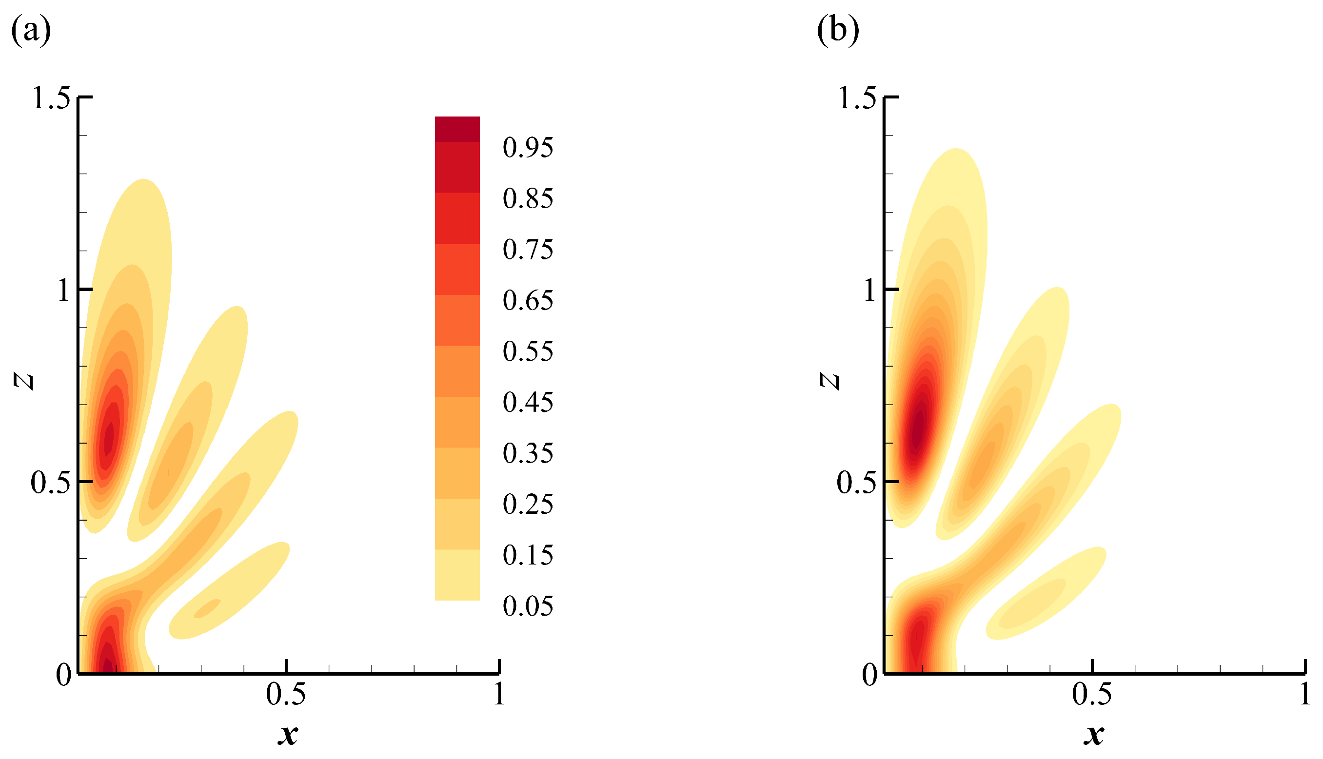
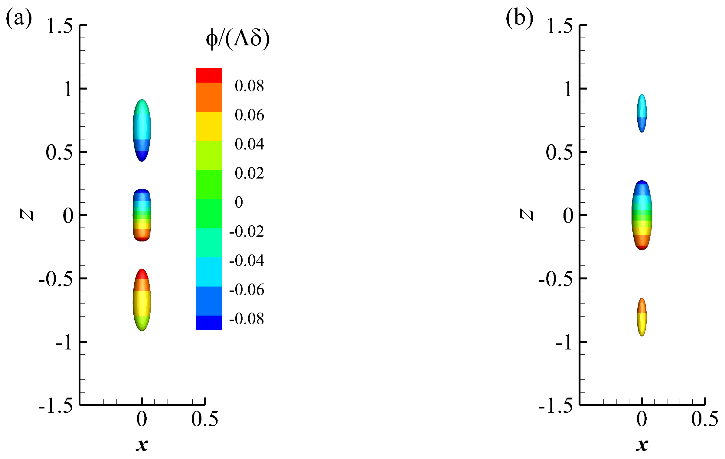
2.2. Analytical Study of a Single Eddy

Following Davidson et al. [18], we consider the evolution of an eddy in a stratified fluid under rotation, assuming that the process is axisymmetric with respect to the eddy axis. In this context, in a cylindrical coordinate system $(r,\theta ,z)$, an axisymmetric velocity field $\mathit{u}$ can be decomposed into azimuthal and poloidal components

$$\mathit{u}=\left(\Gamma /r\right){\mathit{e}}_{\theta }+\nabla \times \left[\left(\psi /r\right){\mathit{e}}_{\theta }\right],$$

(9)

where $\Gamma =u_{\theta }r$ is the angular momentum and $\psi$ is the Stokes streamfunction. We substitute Equation (9) into the linearized inviscid vorticity Equation (4) and the linearized non-diffusive Equation (5) to obtain

$$\frac{\partial \Gamma }{\partial t}=2\Omega \frac{\partial \psi }{\partial z},\frac{\partial }{\partial t}\left(r{\omega }_{\theta }\right)=2\Omega \frac{\partial \Gamma }{\partial z}+Nr\frac{\partial \varphi }{\partial r},\frac{\partial \varphi }{\partial t}=\frac{N}{r}\frac{\partial \psi }{\partial r},$$

(10)

where ${\nabla }_{*}^2\psi =\left(r\partial /\partial r\right)\left(r^{-1}\partial \psi /\partial r\right)+{\partial }^2\psi /\partial z^2=-r{\omega }_{\theta }$, ${\nabla }_{*}^2$ being the Stokes operator. Combining the equations in (10) yields

$$\frac{\partial }{\partial t}\left(\frac{{\partial }^2}{\partial t^2}{\nabla }_{*}^2\Gamma +\left[{\left(2\Omega \right)}^2\frac{{\partial }^2}{\partial z^2}+N^2\left(r\frac{\partial }{\partial r}\right)\left(\frac{\partial }{r\partial r}\right)\right]\Gamma \right)=0.$$

(11)

Equation (11) can be readily solved by using the Hankel-cosine transform

$${\widehat{u}}_{\theta }=\frac{1}{2{\pi }^2}{\int }_0^{\infty }{\int }_0^{\infty }r{u}_{\theta }{J}_1\left(k_{r}r\right)cos\left(k_{z}z\right)\mathrm{d}r\mathrm{d}z,$$

(12)

where $J_1$ is the Bessel function of the first kind of order 1. Here, $k_r$ and $k_z$ represent the wavenumbers in the r-direction and the z-direction, respectively, with $0\le k_r,k_z<\infty$. Given the initial conditions ${\widehat{u}}_{\theta }={\widehat{u}}_{\theta }^{\left(0\right)}$, $\psi =0$ and $\varphi =0$, we can derive that

$${\widehat{u}}_{\theta }=\left[{\widehat{u}}_{\theta }^{\left(0\right)}/\left(N^2{k}_r^2+{\left(2\Omega \right)}^2{k}_z^2\right)\right]\left[N^2{k}_r^2+{\left(2\Omega \right)}^2{k}_z^{2}cos\left(\sqrt{N^2{k}_r^2+{\left(2\Omega \right)}^2{k}_z^2}t/k\right)\right],$$

(13)

from which we obtain

$$\begin{array}{cc}\hfill u_{\theta }=& \underset{\mathrm{PV}\mathrm{mode}}{\underbrace{4\pi {\int }_0^{\infty }{\int }_0^{\infty }\left(N^2{k}_r^3{\widehat{u}}_{\theta }^{\left(0\right)}/{\alpha }^2\right)J_1\left(k_{r}r\right)cos\left(k_{z}z\right)\mathrm{d}{k}_r\mathrm{d}{k}_z}}\hfill \\ \hfill & +\underset{\mathrm{inertial}-\mathrm{gravity}\mathrm{waves}}{\underbrace{2\pi {\int }_0^{\infty }{\int }_0^{\infty }\left[{\left(2\Omega \right)}^2{k}_r{k}_z^2{\widehat{u}}_{\theta }^{\left(0\right)}/{\alpha }^2\right]J_1\left(k_{r}r\right)\left[cos\left(k_{z}z-\alpha t/k\right)+cos\left(k_{z}z+\alpha t/k\right)\right]\mathrm{d}{k}_r\mathrm{d}{k}_z}},\hfill \end{array}$$

(14)

where we introduce $\alpha =\sqrt{N^2{k}_r^2+{\left(2\Omega \right)}^2{k}_z^2}$ for conciseness. In the absence of stratification (i.e., when $N=0$), Equations (13) and (14) are consistent with the results presented in Davidson et al. [18], which consider only the rotation of the system. However, the inclusion of stratification introduces a new time-independent term and changes the frequencies of the previously identified wave-like components. Note that the phase velocities of the wave-like components, given by $\pm \alpha /k$, closely match those of the inertial-gravity waves according to Equation (7), provided we replace $k_r$ with $k_h$. This alignment strongly suggests that these wave-like components are indeed manifestations of the inertial-gravity waves. In a spatially uniform rotating stratified flow with periodic boundary condition, Smith and Waleffe [39] identified the linear eigenmodes as two inertial-gravity waves and a PV mode, suggesting that the time-independent term in (14) is consistent with the zero-frequency PV mode. However, our solution shows how these PV mode and inertial-gravity waves manifest in the flow evolution from a spatially localized initial condition—an aspect not addressed in previous studies. Later in Section 2.3, we will explore the associated flow structures and elucidate their role in energy dispersion.

2.3. Numerical Validation of the Analytical Results

To assess the applicability of the analytical results in Section 2.2 and to develop a better understanding of the evolution of a single eddy in a rotating stratified fluid, a simple initial velocity field of the Gaussian-eddy form is chosen:

$$\mathit{u}=\Lambda rexp\left(-\frac{r^2+z^2}{{\delta }^2}\right){\mathit{e}}_{\theta },$$

(15)

for which Davidson et al. [18] have given an analytical solution when only the rotation is considered. In this equation, $\Lambda$ is the characteristic angular rotation rate and $\delta$ is the characteristic size. The corresponding Rossby and Froude numbers are defined by $Ro=\Lambda /\left(2\Omega \right)$ and $Fr=\Lambda /N$, respectively. To validate our analytical solutions, we chose parameters $Ro=0.02$ and $Fr=0.16$, corresponding to a vortex characterized by $\Lambda =0.422$ and $\delta =0.125$. This choice corresponds to a parameter set from our turbulent cloud studies in Section 3. We note that the validation of our analytical solutions remains robust across different parameter sets in these studies. The analytical solution is obtained by substituting (15) into (14). We then performed a DNS to study the evolution of this Gaussian eddy. Equations (1)–(3) are solved using a parallelized pseudo-spectral code in a ${512}^3$ periodic box of size $l_{box}=2\pi$, where the fourth-order Runge–Kutta time-stepping scheme is employed [40]. The linear terms caused by rotation and stratification, together with the viscous and diffusive terms, are integrated exactly by using an integrating factor technique. A combination of phase-shifting and truncation is used to de-alias the nonlinear terms (see e.g., Ref. [41]).

Figure 1a,b show the contours of $u_{\theta }^2$ (normalized by its maximum value) in the x-z plane passing through the axis of the Gaussian eddy at $t/t_f=13.5$. These are results from the analytical solution and the DNS, respectively. Here $t_f=1/\left(2\Omega \right)$ denotes the rotation time scale. The DNS result, which considers the full Navier–Stokes equations including viscous and nonlinear effects, is still in close agreement with the analytical counterpart. Although there are discrepancies due to these effects, the overall trend and structure are consistent between the two. A prominent region of $u_{\theta }^2$ near the origin stands out, which is absent in the unstratified scenario (Ref. [19], Figure 3). This region is indicative of the PV mode, while the other intense regions represent inertial-gravity waves.

To illustrate the evolution of the flow structures and their corresponding energy dispersion, Figure 2 shows iso-surfaces of the vertical vorticity, ${\omega }_z=0.1\Lambda$, color-coded with $\varphi$, at times $t/t_f=13.5$ and $16.9$. As the system begins to evolve, a central vortex appears at the origin, flanked by two vortices, one above and one below (Figure 2a). Over time, the central vortex undergoes minor changes, while the flanking vortices become smaller and their centers move further away from the origin (Figure 2b). This behavior is in stark contrast to the purely rotating case [34], where only two columnar structures emerge, progressively moving away from each other as they elongate. The shifts in the flow structures can be attributed to the interplay between the Coriolis and buoyancy forces. In Figure 2a, all three cyclonic vortices ($w_z>0$) are influenced by the Coriolis force, causing them to stretch horizontally. For the central vortex, $\varphi$ has negative values at the top and positive ones at the base. This distribution results in a vertical stretch from the buoyancy force, which causes a horizontal contraction of the vertex due to the incompressibility of the fluid, counteracting the Coriolis force. As a result, this vortex remains relatively stable, maintaining a nearly consistent energy distribution over time. For each flanking vortex, $\varphi$ retains its sign, showing larger absolute values for smaller magnitudes of $\left|z\right|$. This implies that the buoyancy force is acting to move these vortices away from the origin and to compress them vertically. The interaction of the Coriolis and buoyancy forces causes these vortices to recede and decrease in size, resulting in energy dispersion and potential-kinetic energy exchange. It is worth noting that a similar phenomenon to the central vortex has been documented in fully developed rotating stratified turbulence, where it correlates with a pronounced exchange between kinetic and potential energy [40].

3. A Stratified Turbulent Cloud under Rotation

In this section, we move from the study of a single eddy to the nonlinear evolution of a turbulent cloud. We observe characteristics compatible with inertial-gravity waves in DNS by studying the flow structures. Finally, we calculate the energy exchanged from the turbulent cloud by these waves to understand their role in energy transfer for localized turbulent patches.

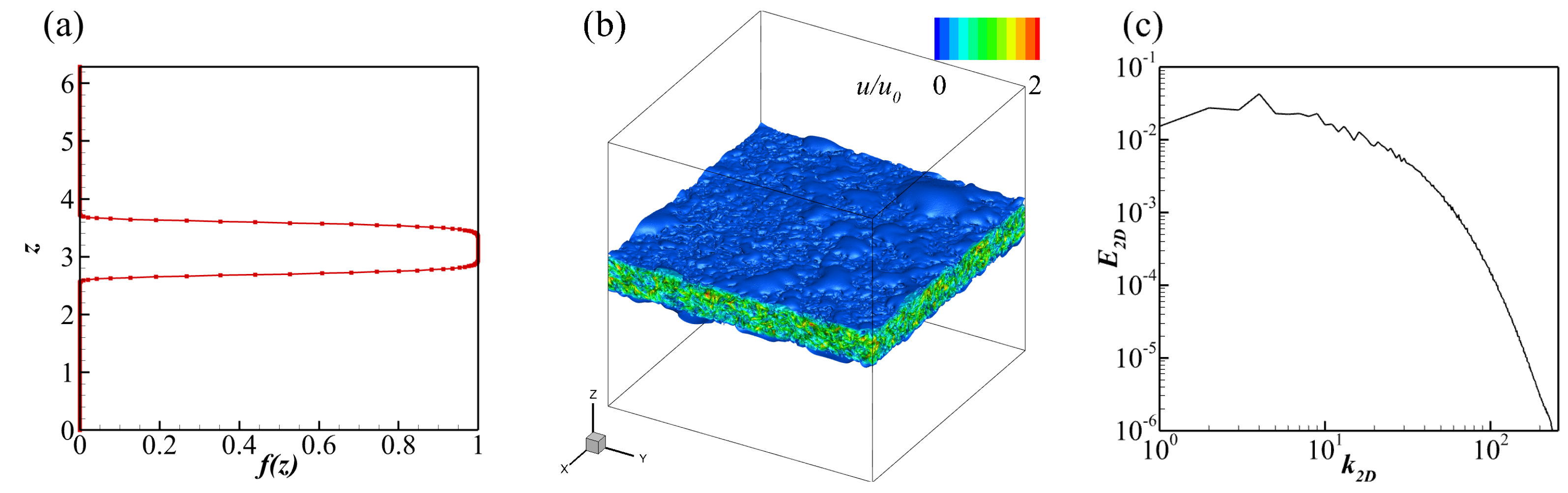
3.1. DNS of a Turbulent Cloud

Following the procedure described by Ranjan and Davidson [19], we performed DNS on fully developed homogeneous isotropic turbulence to obtain the initial velocity field for the turbulent cloud study. We then selected a velocity field corresponding to a specific moment characterized by an integral length scale of $l_0\sim {\int }_0^{\infty }{k}^{-1}E\left(k\right)\mathrm{d}k/{\int }_0^{\infty }E\left(k\right)\mathrm{d}k\approx 0.04l_{box}$ and a Reynolds number $R{e}_0=u_0{l}_0/\nu \approx 169$, where $E\left(k\right)$ is the energy spectrum and $u_0$ is the r.m.s. velocity. To numerically generate a horizontal turbulent cloud, the resulting velocity field was spatially filtered with

$$f\left(z\right)=exp\left(-{10}^a{\left|z-\pi \right|}^m\right),$$

(16)

as shown in Figure 3a. Here we set $a=4$ and $m=9$, resulting in a cloud thickness of $l_c=0.13l_{box}$, approximately three times the integral length scale $l_0$. The velocity field is then projected to be divergence-free. The buoyancy field was initialized with $\varphi =0$ throughout the computational domain, which ensures a uniformly linear density profile, indicating no initial mixing within the cloud. Figure 3b shows the initial turbulent cloud as indicated by the velocity module, and its spectrum in the x-y plane, averaged over its central part in the z-direction, is shown in Figure 3c.

To investigate the effect of the stratification on the evolution of a turbulent cloud under rotation, we conducted DNS with a constant Rossby number, $Ro=0.11$, and five different Froude numbers: $Fr=\infty$ (corresponding to $N=0$, a purely rotating scenario), $0.88$, $0.44$, $0.22$ and $0.11$. All simulations started from the same initial condition with no external forcing (i.e., the decaying case). The simulation parameters are given in

Table 1. Simulation parameters for the DNS of a turbulent cloud. In all cases, we have set $\nu =\kappa =0.001$.

Case	Resolution	$\mathit{Ro}$	$2\mathit{\Omega }$	$\mathit{Fr}$	N	$\mathit{Bu}$	${\mathit{Re}}_0$	${\mathit{l}}_{\mathit{c}}/{\mathit{l}}_{\mathit{box}}$	${\mathit{l}}_{\mathit{c}}/{\mathit{l}}_0$
R0.11	${512}^3$	0.11	21.1	∞	0.0	0.00	169	0.13	3
F0.88	${512}^3$	0.11	21.1	0.88	2.6	0.02	169	0.13	3
F0.44	${512}^3$	0.11	21.1	0.44	5.3	0.06	169	0.13	3
F0.22	${512}^3$	0.11	21.1	0.22	10.6	0.25	169	0.13	3
F0.11	${512}^3$	0.11	21.1	0.11	21.1	1.00	169	0.13	3

, where $Ro=u_0/\left(2\Omega l_0\right)$ and $Fr=u_0/\left(N{l}_0\right)$. With the exception of the purely rotating case R0.11, the simulations are denoted by their Froude numbers, e.g., the case F0.88 corresponds to $Fr=0.88$. For practical reference, we have also listed the Burger number, $Bu={(Ro/Fr)}^2$ [42], for each case in Table 1. This number indicates the balance between stratification and rotation in the flows studied.

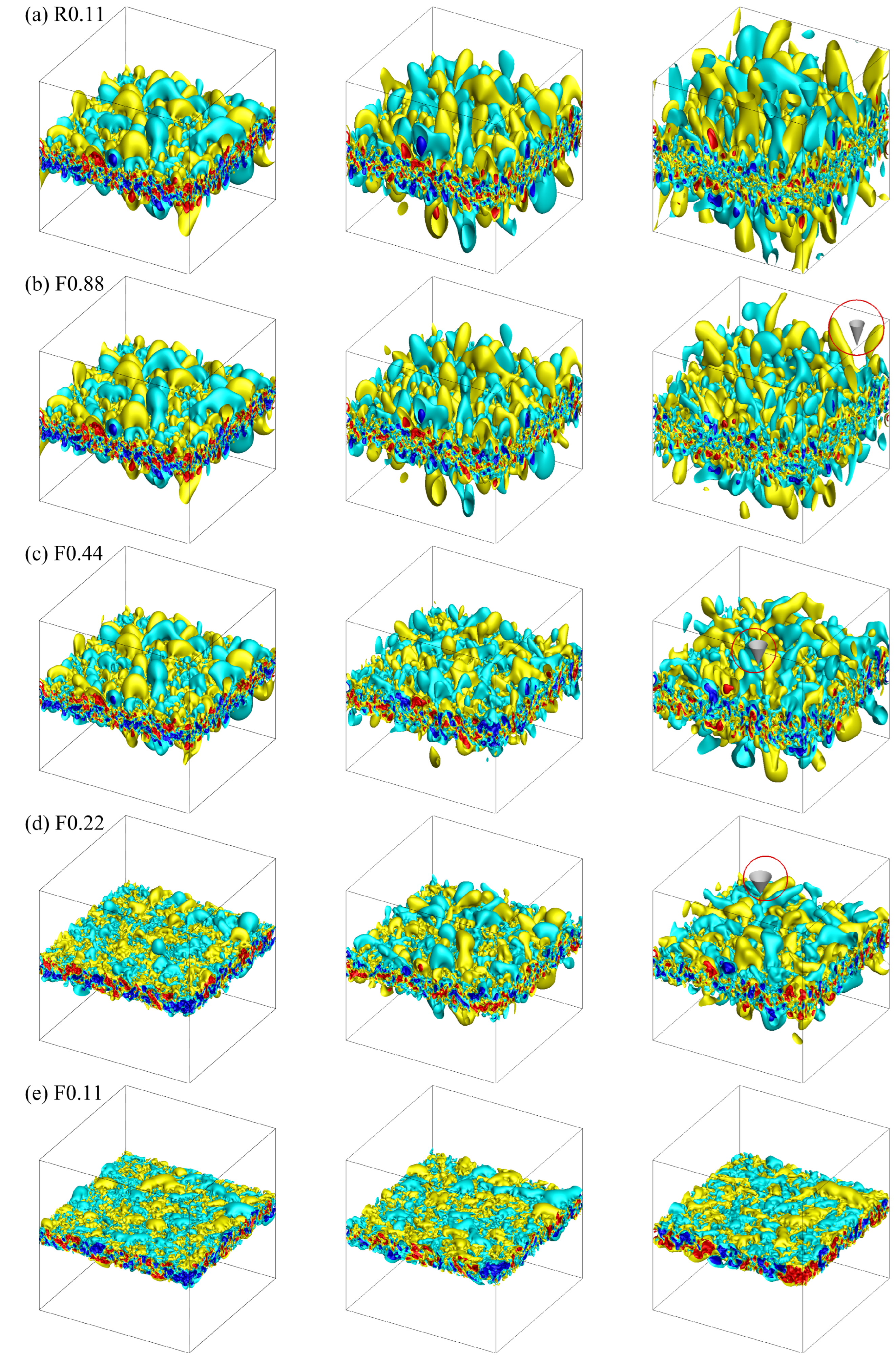
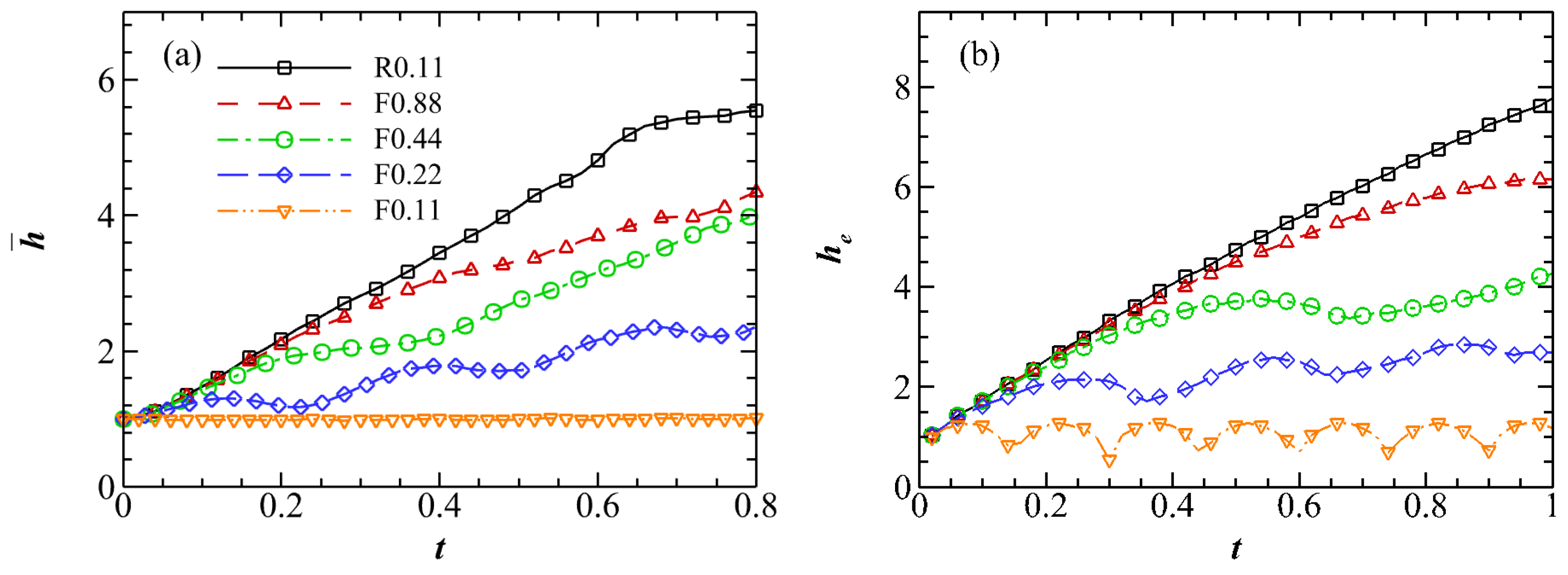
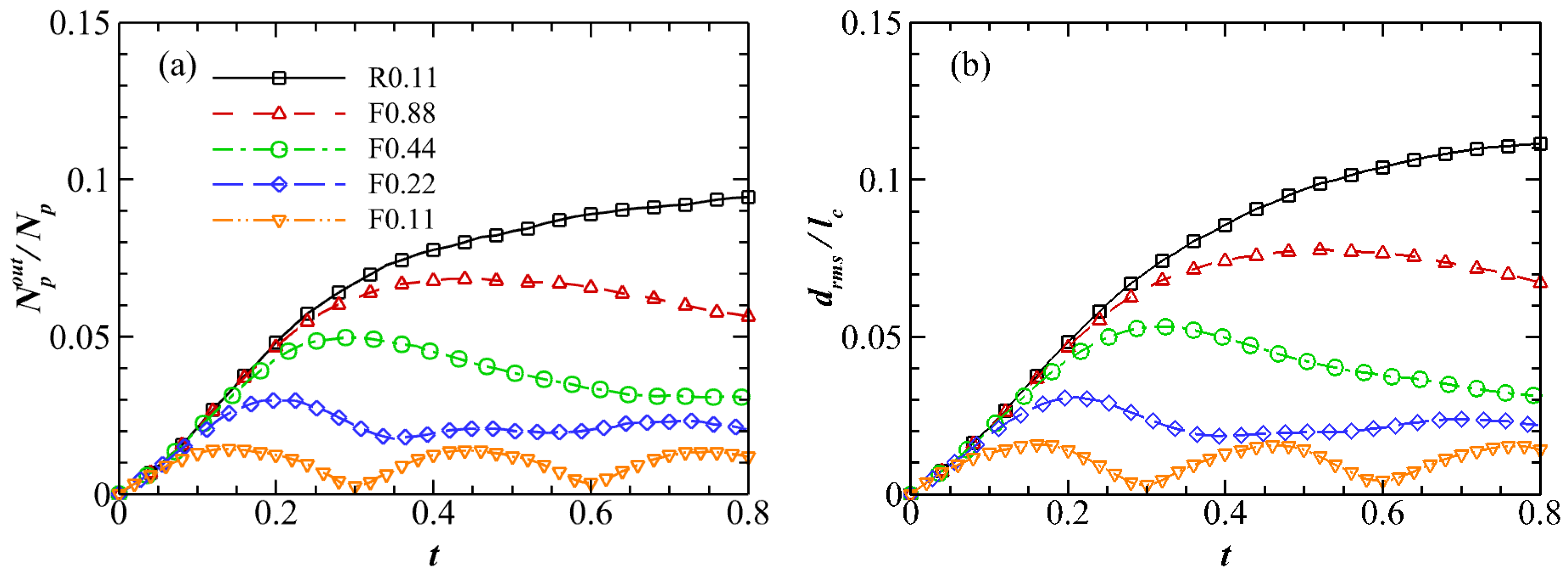
3.2. Evolution of Flow Structures

To show the evolution of the turbulent cloud structures, Figure 4 shows iso-surfaces of $u_z$ for all simulations at different times. For the case R0.11 under pure rotation, Figure 4a shows the emergence of vertical columnar structures from the turbulent cloud, which extend into the quiescent region, in agreement with previous experimental results [18] and numerical study [19]. For the weakly stratified case F0.88, Figure 4b shows subtle differences in the flow structures at $t/t_f=8.4$ (middle panels) and more pronounced variations at $t/t_f=12.7$ (right panels) compared to the case R0.11.

For the moderately stratified cases F0.44 and F0.22, Figure 4c,d show that the columnar structures tend to deviate from a purely vertical orientation as they extend into the quiescent region. This tilt becomes more pronounced with increasing stratification. A comparison of Figure 4a–e shows that, at equivalent time intervals, the vertical growth of these structures decreases with decreasing $Fr$. This suggests that strong density stratification limits the vertical expansion of the cloud, consistent with the observation in experiments [31].

In the case F0.11 (Figure 4e), the rotation frequency and the Brunt–Väisälä frequency are identical. As a result, no structures emerge from the turbulent cloud, suggesting minimal energy emission from the cloud. This behavior mirrors the case without both rotation and stratification, as documented in Ref. [19]. A plausible interpretation is that the stratification strength is sufficient to completely inhibit the vertical expansion of the turbulent cloud in the presence of system rotation. It is noteworthy that Equation (7) for this scenario yields $\varpi =2\Omega =N$, implying uniform frequencies of inertial-gravity waves in all directions. This monochromatic behavior is consistent with systems in which both rotation and stratification are absent.

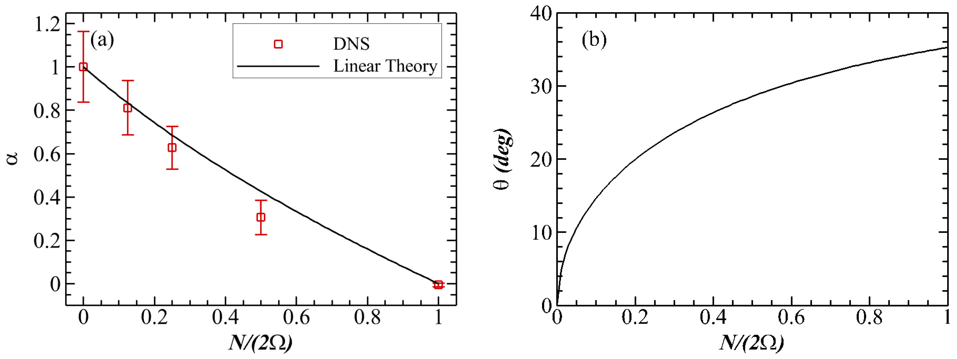
3.3. Are the Flow Structures Formed by Inertial-Gravity Waves?

Columnar structures from a turbulent cloud under rotation have been identified as inertial waves [19], while the large-scale pancake structures from a stratified turbulent cloud are recognized as internal gravity waves [26]. This section examines whether the flow structures discussed in Section 3.2 from the stratified turbulent cloud under rotation can be attributed to inertial-gravity waves.

In all simulations, the growth of flow structures in different directions leads to the expansion of turbulent clouds in the vertical direction, which can be quantified by tracking the boundary of the $|u_z|$ iso-surfaces with time. The reason we choose $u_z$ to indicate structure is that it satisfies the wave equation as described by (6). In particular, given a threshold $|u_z^b|$, the upper and lower boundaries of the cloud can be obtained from the positions where $|u_z|=|u_z^b|$. We can therefore calculate the vertical extent of the cloud, $h(x,y,t)$, for each point on the x-y plane and time t. The mean wave-cloud thickness $\overline{h}\left(t\right)$ is defined as the average of $h(x,y,t)$ over x and y. Figure 5a shows the mean wave-cloud thickness for all the simulations where we choose $|u_z^b|=0.35u_0$. The results remain robust when the threshold varies around this value, and this threshold is used consistently throughout the analysis in this paper. For the purely rotating case R0.11, the mean wave-cloud thickness shows a linear growth with time, resulting from the inertial waves with $k_z=0$ traveling at the group velocity $c_g=2\Omega ⁄k_h$ [19]. For the case F0.88 with weak stratification, the mean wave-cloud thickness is close to that in the case R0.11 at $t\le 0.2$, indicating that the stratification does not affect the cloud before $t=0.2$. This is because the linear time scale corresponding to the rotation, $t_f=1/\left(2\Omega \right)$, is smaller than that corresponding to the stratification, $t_N=1/N$. When $t>0.2$, the mean wave-cloud thickness shows a smaller linear growth rate. For the cases F0.44 and F0.22 with stronger stratification, the behavior of the mean wave-cloud thicknesses can be interpreted as the superposition of a linear growth and an oscillation with a fixed frequency over time. In addition, the frequency is larger in the case F0.22. The mean wave-cloud thickness in the case F0.11 is almost constant with time, which is consistent with the observation in Figure 4e.

To investigate whether the flow structures are closely related to the inertial-gravity waves, we compare the results from the DNS with those predicted by the linear theory. Since the initial turbulent cloud can be viewed as a distribution of random vortex blobs of different shapes and sizes, we consider the linear evolution of a Gaussian vortex satisfying Equation (15) under the same Rossby and Froude numbers. We set $\Lambda =2.31$, $\delta =0.125$, and utilize $|u_z^b|=0.002\Lambda \delta$ to determine the vertical extent of the eddy, $h_e$. This extent is defined as the largest vertical distance between the positions where $|u_z|=|u_z^b|$. Figure 5b shows that the results for $h_e$ align qualitatively with those of $\overline{h}$ in Figure 5a, suggesting that the expansion of the turbulent cloud may be prominently influenced by the linear mechanism. Note that the difference for the case F0.11, where the curve appears flat in Figure 5a and wave-like in Figure 5b, arises because $\overline{h}$ represents an average over various x and y, whereas $h_e$ illustrates the results for a single eddy.

We now show quantitatively that the flow structures are closely related to inertial-gravity waves. For a vortex blob in the initial turbulent cloud, we suppose that it is characterized by a length scale of $1/k$. Then its rescaled group velocity in the vertical direction is

$${\tilde{c}}_{g,z}=k{c}_{g,z}=\pm \frac{2\Omega (1-{(N/\left(2\Omega \right))}^2)(k_z/k_h)}{\sqrt{{(N/\left(2\Omega \right))}^2+{(k_z/k_h)}^2}(1+{(k_z/k_h)}^2)}.$$

(17)

Given the ratio of the Brunt–Väisälä frequency to the rotation frequency $N/\left(2\Omega \right)$, it is determined that when

$${\left(\frac{k_z}{k_h}\right)}^2=\frac{1}{4}\left[-{(N/\left(2\Omega \right))}^2+\sqrt{{(N/\left(2\Omega \right))}^4+8{(N/\left(2\Omega \right))}^2}\right],$$

(18)

${\tilde{c}}_{g,z}$ reaches the maximum ${\tilde{c}}_{g,z}^{max}$, which is the vertical growth rate of the turbulent cloud predicted by the linear inertial-gravity waves. Furthermore, the corresponding value of $k_z/k_h={(k_z/k_h)}_0$ characterizes the tilt angle of the flow structure. The vertical growth rate of the turbulent cloud in the DNS can be determined from the growth rate of the mean wave-cloud thickness, $\overline{h}\left(t\right)$, as shown in Figure 5a. The rate is calculated using a linear fitting method. In Figure 6a we present two vertical growth rates: ${\alpha }_{DNS}$ derived from DNS and ${\alpha }_{LT}$ derived from linear theory. To facilitate comparison, both rates are normalized by their values at $N/2\Omega =0$. Figure 6b shows the angle between the flow structure and the vertical direction, $\theta =arctan\left[{(k_z/k_h)}_0\right]$, predicted by linear theory for different $N/\left(2\Omega \right)$. The results are consistent with Figure 4, where the angle becomes larger as $N/\left(2\Omega \right)$ increases. For quantitative comparison, we also plot cones in the third columns of Figure 4b–d, where the angle between the cone surface and the vertical axis is equal to $\theta$. It is notable that there is a strong agreement between the DNS results and the predictions of linear theory. However, for the case F0.22, both $\alpha$ and $\theta$ are slightly underestimated by the linear theory. This discrepancy could be due to the interactions between waves and turbulence, especially given the small vertical expansion of the cloud in this case. It is important to note that in scenarios where both rotation and stratification are present, the frequency of the inertial-gravity waves (7) tied to ${\tilde{c}}_{g,z}^{max}$ is not zero. This explains the oscillatory component observed in $\overline{h}$ for the cases F0.44 and F0.22. When only rotation or stratification is present, the maximum group velocity always coincides with inertial (or gravity) waves of zero frequency. Under these circumstances, tools such as two-dimensional energy spectrum analysis can be used effectively, given the consistent phase of $u_z$ [19] or $u_x$ [26] at the edge of the turbulent cloud.

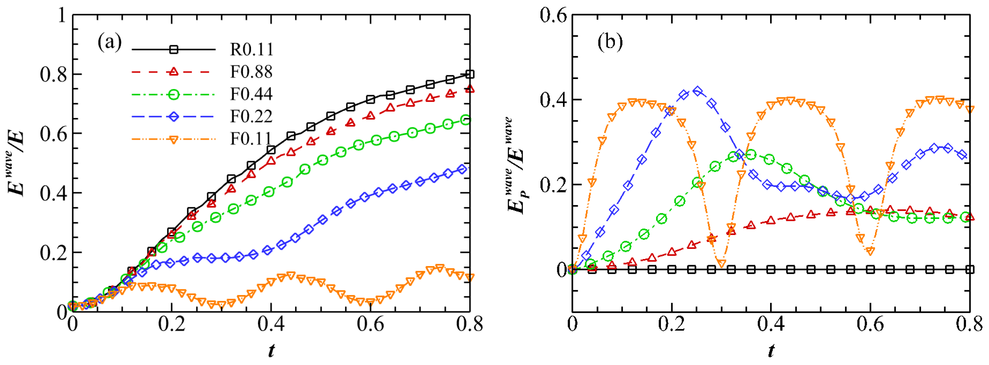
3.4. Wave-Dominated and Turbulence-Dominated Regions

In Section 3.3 it is highlighted that the flow structures emerging from the turbulent cloud show a strong association with inertial-gravity waves. In stratified turbulence, PV has been used to identify turbulent/non-turbulent interfaces [26,43]. Our study, however, uses Lagrangian particle tracking to measure the vertical extent of turbulent advection [19]. Lagrangian particles act as passive tracers, with their position $\mathit{r}$ at time t given by $\mathrm{d}\mathit{r}/\mathrm{d}t=\mathit{u}(\mathit{r},t)$. In this relationship, $\mathit{u}$ represents the velocity of the fluid. To determine $\mathit{u}$ at the particle positions, we use a 6th-order Lagrange interpolation. Furthermore, the positions of these particles are integrated using a 2nd-order Adams–Bashforth scheme.

Tracer particles with a number $N_p=65536$ are initialized randomly from a uniform distribution throughout the initial turbulent cloud, the vertical range of which is denoted as $[z_0,z_1]$. Let $N_p^{out}$ be the number of particles outside of the range of the initial turbulent cloud. The r.m.s. distance of these particles to the initial turbulent cloud can be calculated as

$$d_{rms}=\sqrt{\frac{1}{N_p^{out}}\sum _{p=1}^{N_p^{out}}{d}_p^2},$$

(19)

where

$$d_p=\left\{\begin{array}{cc}{z}_p-z_1,\hfill & z_p>z_1\hfill \\ z_0-z_p,\hfill & z_p<z_0\hfill \end{array}\right.$$

(20)

represents the distance of the particle p to the initial turbulent cloud. We consider $[z_0-d_{rms},z_1+d_{rms}]$ as the vertical range of the turbulence-dominated region and the other domain as the wave-dominated region. Figure 7 shows the ratio of particles outside the initial turbulent cloud, $N_p^{out}/N_p$, and $d_{rms}$ normalized with the initial cloud thickness $l_c$. For the case R0.11, both $N_p^{out}/N_p$ and $d_{rms}/l_c$ increase with time, while for the cases F0.88 and F0.44 both quantities first increase and then decrease after reaching the maximum values, likely approaching a stationary state due to the stable stratification. However, in the cases F0.22 and F0.11, where the stratification is strong, both quantities immediately reach stationary states around small values.

Table 2. Maximum proportion of particles located outside the initial turbulent cloud, and the maximum vertical cloud expansion for the different cases.

Case	R0.11	F0.88	F0.44	F0.22	F0.11
$max(N_p^{out}/N_p)$	$9.45\%$	$6.86\%$	$4.98\%$	$2.99\%$	$1.44\%$
$max(d_{rms}/l_c)$	$11.16\%$	$7.77\%$	$5.33\%$	$3.08\%$	$1.57\%$

presents the maximum values of $N_p^{out}/N_p$ and $d_{rms}/l_c$ for all cases, where $max(d_{rms}/l_c)$ can also be interpreted as the maximum vertical expansion of the initial turbulent cloud. It is observed that both quantities become smaller with increasing stratification, indicating the limitation of vertical turbulent advection by stratification.

Once the regions dominated by waves and turbulence are identified, we can determine the energy of the turbulent cloud carried away by the inertial-gravity waves, denoted as $E^{wave}$. This energy is equal to the energy within the wave-dominated region. Figure 8a shows that for cases where $Ro<Fr$, the ratio $E^{wave}/E$ exhibits a monotonic increase with time. In particular, for a given time point, a decrease in $Fr$ results in smaller values of $E^{wave}/E$. This suggests that under stronger stratification, inertial-gravity waves contain a smaller fraction of the energy. In contrast, for the scenario where $Ro=Fr$, the ratio $E^{wave}/E$ oscillates with a fixed pattern. Its values fluctuate between nearly zero and a peak of about $15\%$, indicating that the inertial-gravity waves only sporadically extract a small fraction of energy from the turbulent cloud. Thus, while inertial waves account for a significant fraction of the energy in a system dominated by rotation alone, this energy contribution diminishes with the introduction of stratification. Figure 8b shows the ratio of potential energy to total energy in the wave-dominated region, $E_P^{wave}/E^{wave}$. As stratification increases, potential energy becomes increasingly dominant and varies more frequently with time. This highlights the increasing importance of the kinetic-potential energy exchange and suggests that the dominant inertial-gravity waves exhibit greater phase velocities under increased stratification. It is worth noting that a similar kinetic-potential energy exchange phenomenon has been reported in fully developed rotating stratified turbulence [44].

4. Discussion and Conclusions

In this study, we investigate the evolution of a stratified turbulent cloud influenced by rotation. By analyzing the behavior of a single eddy under both rotation and stratification, we observe clear deviations from the purely rotating scenario. In particular, within the stratified environment, we detect a spatial manifestation of a known PV mode, characterized as a stable vortex at the origin. Furthermore, the system transitions from exhibiting inertial waves to producing inertial-gravity waves, whose propagation relations depend on both rotation and stratification.

Numerical simulations have been performed to investigate the nonlinear evolution of the turbulent cloud influenced by different degrees of stratification under rotation. In cases where $Ro<Fr$, columnar structures emerge spontaneously from the turbulent cloud. These structures are vertically oriented in the case of pure rotation, but deviate from the vertical as stratification is introduced. As $Fr$ decreases, the tilt angle increases and the rate of cloud expansion decreases. Conversely, in the $Ro=Fr$ system, the turbulent cloud remains devoid of distinct structures, reminiscent of scenarios without rotation and stratification. The flow structures are observed to have characteristics consistent with inertial-gravity waves. This observation is supported by the agreement between DNS and linear theory, which gives consistent predictions for the vertical growth rates of the turbulent cloud and the tilt angles of these structures. Using Lagrangian particle tracking, we distinguish between wave-dominated and turbulence-dominated regions. It is found that the inertial gravity waves emitted by the cloud can transport a substantial fraction of the energy to the neighboring quiescent fluid, which decreases with increasing stratification. This suggests the central role of inertial-gravity waves in energy transfer processes within atmospheres and oceans, particularly around regions of localized turbulence.

The present study elucidates the effects of stratification on localized turbulence under system rotation. First, compared to the purely rotating case, the presence of stratification introduces the zero-frequency PV mode, whose energy distribution barely changes with time. While this mode is not new, our finding is its distinct spatial manifestation within a non-uniformly turbulent background. Second, as the stratification intensifies, the dominant inertial-gravity waves exhibit increased tilting and reduced vertical group velocity. In combination, these phenomena limit the energy emitted by the initial turbulent cloud. It should be noted that this study focuses on the parameter regime where $Ro<Fr$ (the corresponding $Bu$ ranges from 0 to 1). While the $Ro>Fr$ regime is thought to dominate in the Earth’s atmosphere and oceans [7], the $Ro<Fr$ regime is relevant for several geophysical flows, such as in the deep sea where the influence of stratification is weak but rotation effects are prominent [45,46,47,48,49].

There are still many open questions that need to be addressed. Specifically, the potential role of the Ro/Fr ratio in influencing the flow dynamics and the effect of the Reynolds number warrant further investigation [50,51]. Previous research has shown that the absence of triadic resonance in the parameter range $1/2\le N/\left(2\Omega \right)\le 2$ is associated with an enhanced inverse cascade [39,50]. The particular significance of this range requires further investigation. In addition, the pronounced enhancement of vertical velocity, termed “vertical drafts”, is a common observation in many DNS studies of stratified flows [52,53] and in the oceans [54]. We did not detect such vertical drafts in our simulations, which may be due to the initialization from homogeneous isotropic turbulence rather than rotating stratified turbulence, or the Froude numbers considered are not favorable for such a phenomenon. Given its importance, this phenomenon is worthy of systematic investigation for the development of turbulent clouds in the future. Furthermore, the study of the corresponding Lagrangian statistics is another interesting research direction [55].

References

1. Grant, H.; Moilliet, A.; Vogel, W. Some observations of the occurrence of turbulence in and above the thermocline. J. Fluid Mech. 1968, 34, 443–448. [Google Scholar] [CrossRef]
2. Nasmyth, P.W. Oceanic Turbulence. Ph.D. Thesis, University of British Columbia, Vancouver, BC, Canada, 1970. [Google Scholar]
3. Wijesekera, H.W.; Dillon, T.M. Internal waves and mixing in the upper equatorial Pacific Ocean. J. Geophys. Res. Ocean. 1991, 96, 7115–7125. [Google Scholar] [CrossRef]
4. Nash, J.; Alford, M.; Kunze, E.; Martini, K.; Kelly, S. Hotspots of deep ocean mixing on the Oregon continental slope. Geophys. Res. Lett. 2007, 34, L01605. [Google Scholar] [CrossRef]
5. Davidson, P. Turbulence: An Introduction for Scientists and Engineers; Oxford University Press: Oxford, UK, 2015. [Google Scholar]
6. Yang, C.F.; Chi, W.C.; van Haren, H. Deep-sea turbulence evolution observed by multiple closely spaced instruments. Sci. Rep. 2021, 11, 3919. [Google Scholar] [CrossRef] [PubMed]
7. Riley, J.J.; Lelong, M.P. Fluid motions in the presence of strong stable stratification. Annu. Rev. Fluid Mech. 2000, 32, 613–657. [Google Scholar] [CrossRef]
8. Sutherland, B.R. Internal Gravity Waves; Cambridge University Press: Cambridge, UK, 2010. [Google Scholar]
9. Thorpe, S.A. The Turbulent Ocean; Cambridge University Press: Cambridge, UK, 2005. [Google Scholar]
10. Yarom, E.; Sharon, E. Experimental observation of steady inertial wave turbulence in deep rotating flows. Nat. Phys. 2014, 10, 510–514. [Google Scholar] [CrossRef]
11. Buzzicotti, M.; Aluie, H.; Biferale, L.; Linkmann, M. Energy transfer in turbulence under rotation. Phys. Rev. Fluids 2018, 3, 034802. [Google Scholar] [CrossRef]
12. Alexakis, A.; Biferale, L. Cascades and transitions in turbulent flows. Phys. Rep. 2018, 767, 1–101. [Google Scholar] [CrossRef]
13. Di Leoni, P.C.; Alexakis, A.; Biferale, L.; Buzzicotti, M. Phase transitions and flux-loop metastable states in rotating turbulence. Phys. Rev. Fluids 2020, 5, 104603. [Google Scholar] [CrossRef]
14. Savaro, C.; Campagne, A.; Linares, M.C.; Augier, P.; Sommeria, J.; Valran, T.; Viboud, S.; Mordant, N. Generation of weakly nonlinear turbulence of internal gravity waves in the Coriolis facility. Phys. Rev. Fluids 2020, 5, 073801. [Google Scholar] [CrossRef]
15. Monsalve, E.; Brunet, M.; Gallet, B.; Cortet, P.P. Quantitative experimental observation of weak inertial-wave turbulence. Phys. Rev. Lett. 2020, 125, 254502. [Google Scholar] [CrossRef] [PubMed]
16. Hopfinger, E.; Browand, F.; Gagne, Y. Turbulence and waves in a rotating tank. J. Fluid Mech. 1982, 125, 505–534. [Google Scholar] [CrossRef]
17. Dickinson, S.C.; Long, R.R. Oscillating-grid turbulence including effects of rotation. J. Fluid Mech. 1983, 126, 315–333. [Google Scholar] [CrossRef]
18. Davidson, P.; Staplehurst, P.; Dalziel, S. On the evolution of eddies in a rapidly rotating system. J. Fluid Mech. 2006, 557, 135–144. [Google Scholar] [CrossRef]
19. Ranjan, A.; Davidson, P. Evolution of a turbulent cloud under rotation. J. Fluid Mech. 2014, 756, 488–509. [Google Scholar] [CrossRef]
20. Thorpe, S. On the layers produced by rapidly oscillating a vertical grid in a uniformly stratified fluid. J. Fluid Mech. 1982, 124, 391–409. [Google Scholar] [CrossRef]
21. Browand, F.; Guyomar, D.; Yoon, S.C. The behavior of a turbulent front in a stratified fluid: Experiments with an oscillating grid. J. Geophys. Res. Ocean. 1987, 92, 5329–5341. [Google Scholar]
22. De Silva, I.; Fernando, H. Some aspects of mixing in a stratified turbulent patch. J. Fluid Mech. 1992, 240, 601–625. [Google Scholar] [CrossRef]
23. De Silva, I.; Fernando, H.J. Experiments on collapsing turbulent regions in stratified fluids. J. Fluid Mech. 1998, 358, 29–60. [Google Scholar] [CrossRef]
24. Gilreath, H.; Brandt, A. Experiments on the generation of internal waves in a stratified fluid. AIAA J. 1985, 23, 693–700. [Google Scholar] [CrossRef]
25. Rowe, K.; Diamessis, P.; Zhou, Q. Internal gravity wave radiation from a stratified turbulent wake. J. Fluid Mech. 2020, 888, A25. [Google Scholar] [CrossRef]
26. Maffioli, A.; Davidson, P.; Dalziel, S.; Swaminathan, N. The evolution of a stratified turbulent cloud. J. Fluid Mech. 2014, 739, 229–253. [Google Scholar] [CrossRef]
27. Veronis, G. The analogy between rotating and stratified fluids. Annu. Rev. Fluid Mech. 1970, 2, 37–66. [Google Scholar] [CrossRef]
28. Pedlosky, J. Geophysical Fluid Dynamics; Springer: New York, NY, USA, 2013. [Google Scholar]
29. Vallis, G.K. Atmospheric and Oceanic Fluid Dynamics; Cambridge University Press: Cambridge, UK, 2017. [Google Scholar]
30. Manins, P. Intrusion into a stratified fluid. J. Fluid Mech. 1976, 74, 547–560. [Google Scholar] [CrossRef]
31. Davies, P.A.; Fernando, H.J.; Besley, P.; Simpson, R.J. Generation and spreading of a turbulent mixed layer in a rotating, stratified fluid. J. Geophys. Res. Ocean. 1991, 96, 12567–12585. [Google Scholar] [CrossRef]
32. Folkard, A.M.; Davies, P.A.; Fernando, H.J. Measurements in a turbulent patch in a rotating, linearly-stratified fluid. Dyn. Atmos. Ocean. 1997, 26, 27–51. [Google Scholar] [CrossRef]
33. Wells, J.R.; Helfrich, K.R. A laboratory study of localized boundary mixing in a rotating stratified fluid. J. Fluid Mech. 2004, 516, 83–113. [Google Scholar] [CrossRef]
34. Ranjan, A.; Davidson, P. DNS of a Buoyant Turbulent Cloud under Rapid Rotation. In Advances in Computation, Modeling and Control of Transitional and Turbulent Flows; World Scientific: Singapore, 2016; pp. 452–460. [Google Scholar]
35. Emery, W.; Lee, W.; Magaard, L. Geographic and seasonal distributions of Brunt-Väisälä frequency and Rossby radii in the North Pacific and North Atlantic. J. Phys. Ocean. 1984, 14, 294–317. [Google Scholar] [CrossRef]
36. Jones, E.; Rudels, B.; Anderson, L. Deep waters of the Arctic Ocean: Origins and circulation. Deep. Sea Res. Part I Oceanogr. Res. Pap. 1995, 42, 737–760. [Google Scholar] [CrossRef]
37. Woodgate, R.A.; Aagaard, K.; Muench, R.D.; Gunn, J.; Björk, G.; Rudels, B.; Roach, A.; Schauer, U. The Arctic Ocean boundary current along the Eurasian slope and the adjacent Lomonosov Ridge: Water mass properties, transports and transformations from moored instruments. Deep. Sea Res. Part I Oceanogr. Res. Pap. 2001, 48, 1757–1792. [Google Scholar] [CrossRef]
38. Lesieur, M. Turbulence in Fluids: Stochastic and Numerical Modelling; Springer Science & Business Media: Dordrecht, The Netherlands, 1987. [Google Scholar]
39. Smith, L.M.; Waleffe, F. Generation of slow large scales in forced rotating stratified turbulence. J. Fluid Mech. 2002, 451, 145–168. [Google Scholar] [CrossRef]
40. Li, T.; Wan, M.; Wang, J.; Chen, S. Flow structures and kinetic-potential exchange in forced rotating stratified turbulence. Phys. Rev. Fluids 2020, 5, 014802. [Google Scholar] [CrossRef]
41. Canuto, C.; Hussaini, M.Y.; Quarteroni, A.; Thomas, A., Jr. Spectral Methods in Fluid Dynamics; Springer Science & Business Media: Berlin/Heidelberg, Germany, 2012. [Google Scholar]
42. Cushman-Roisin, B.; Beckers, J.M. Introduction to Geophysical Fluid Dynamics: Physical and Numerical Aspects; Academic Press: Waltham, MA, USA, 2011. [Google Scholar]
43. Watanabe, T.; Riley, J.J.; de Bruyn Kops, S.M.; Diamessis, P.J.; Zhou, Q. Turbulent/non-turbulent interfaces in wakes in stably stratified fluids. J. Fluid Mech. 2016, 797, R1. [Google Scholar] [CrossRef]
44. Li, T.; Wan, M.; Wang, J.; Chen, S. Spectral energy transfers and kinetic-potential energy exchange in rotating stratified turbulence. Phys. Rev. Fluids 2020, 5, 124804. [Google Scholar] [CrossRef]
45. Wingate, B.A.; Embid, P.; Holmes-Cerfon, M.; Taylor, M.A. Low Rossby limiting dynamics for stably stratified flow with finite Froude number. J. Fluid Mech. 2011, 676, 546–571. [Google Scholar] [CrossRef]
46. Heywood, K.J.; Garabato, A.C.N.; Stevens, D.P. High mixing rates in the abyssal Southern Ocean. Nature 2002, 415, 1011–1014. [Google Scholar] [CrossRef]
47. Van Haren, H.; Millot, C. Gyroscopic waves in the Mediterranean Sea. Geophys. Res. Lett. 2005, 32, L24614. [Google Scholar] [CrossRef]
48. Timmermans, M.L.; Melling, H.; Rainville, L. Dynamics in the deep Canada Basin, Arctic Ocean, inferred by thermistor chain time series. J. Phys. Oceanogr. 2007, 37, 1066–1076. [Google Scholar] [CrossRef]
49. Timmermans, M.L.; Rainville, L.; Thomas, L.; Proshutinsky, A. Moored observations of bottom-intensified motions in the deep Canada Basin, Arctic Ocean. J. Mar. Res. 2010, 68, 625–641. [Google Scholar] [CrossRef]
50. Marino, R.; Mininni, P.D.; Rosenberg, D.; Pouquet, A. Inverse cascades in rotating stratified turbulence: Fast growth of large scales. Europhys. Lett. 2013, 102, 44006. [Google Scholar] [CrossRef]
51. Rosenberg, D.; Pouquet, A.; Marino, R.; Mininni, P.D. Evidence for Bolgiano-Obukhov scaling in rotating stratified turbulence using high-resolution direct numerical simulations. Phys. Fluids 2015, 27, 055105. [Google Scholar] [CrossRef]
52. Feraco, F.; Marino, R.; Pumir, A.; Primavera, L.; Mininni, P.D.; Pouquet, A.; Rosenberg, D. Vertical drafts and mixing in stratified turbulence: Sharp transition with Froude number. Europhys. Lett. 2018, 123, 44002. [Google Scholar] [CrossRef]
53. Marino, R.; Feraco, F.; Primavera, L.; Pumir, A.; Pouquet, A.; Rosenberg, D.; Mininni, P.D. Turbulence generation by large-scale extreme vertical drafts and the modulation of local energy dissipation in stably stratified geophysical flows. Phys. Rev. Fluids 2022, 7, 033801. [Google Scholar] [CrossRef]
54. D’Asaro, E.A.; Lien, R.C.; Henyey, F. High-frequency internal waves on the Oregon continental shelf. J. Phys. Oceanogr. 2007, 37, 1956–1967. [Google Scholar] [CrossRef]
55. Buaria, D.; Pumir, A.; Feraco, F.; Marino, R.; Pouquet, A.; Rosenberg, D.; Primavera, L. Single-particle Lagrangian statistics from direct numerical simulations of rotating-stratified turbulence. Phys. Rev. Fluids 2020, 5, 064801. [Google Scholar] [CrossRef]
Figure 1. Contours of u θ 2 / ( u θ 2 ) m a x in the x-z plane through the axis of the Gaussian eddy at t / t f = 13.5 . The results are from (a) the analytical solution (14) and (b) the DNS.
Atmosphere 14 01590 g001
Figure 2. The iso-surfaces of ω z = 0.1 Λ (front view) color-coded with ϕ obtained from the DNS at (a) t / t f = 13.5 and (b) t / t f = 16.9 .
Atmosphere 14 01590 g002
Figure 3. (a) The spatial filter given by f z = exp 10 a z π m with a = 4 and m = 9 . (b) Initial turbulent cloud visualized by the velocity module. (c) Energy spectrum in the x-y plane, averaged over different z values around the center of the cloud.
Atmosphere 14 01590 g003
Figure 4. The evolution of the iso-surfaces of u z for the cases: (a) R0.11, (b) F0.88, (c) F0.44, (d) F0.22 and (e) F0.11 at t / t f = 4.2 (left), 8.4 (middle) and 12.7 (right). The color scheme is as follows: 0.24 u 0 in yellow, 0.50 u 0 in red, 0.24 u 0 in cyan, and 0.50 u 0 in blue. Cones (highlighted by red circles) are plotted to indicate the predicted tilt angle of flow structures from the linear theory.
Atmosphere 14 01590 g004
Figure 5. (a) The mean wave-cloud thickness h ¯ of turbulent clouds in the DNS. (b) The vertical extent h e of a Gaussian eddy evolving under the same R o and F r as those in the DNS.
Atmosphere 14 01590 g005
Figure 6. (a) Normalized vertical growth rates of the turbulent cloud, α , obtained from the DNS results and the linear theory. (b) The angle θ between the flow structure and the vertical direction as predicted by the linear theory.
Atmosphere 14 01590 g006
Figure 7. (a) The ratio of particles outside the initial turbulent cloud. (b) The r.m.s. distance of particles outside the initial turbulent cloud to its boundary.
Atmosphere 14 01590 g007
Figure 8. (a) The energy ratio within the inertial-gravity waves. (b) The ratio of potential energy to total energy in the wave-dominated region.
Atmosphere 14 01590 g008