Article

Mean Flow from Phase Averages in the 2D Boussinesq Equations

1
Department of Mathematics and Statistics, University of Exeter, Exeter EX4 4QF, UK
2
Lawrence Livermore National Laboratory, Livermore, CA 94550, USA
*
Author to whom correspondence should be addressed.
Atmosphere 2023, 14(10), 1523; https://doi.org/10.3390/atmos14101523
Submission received: 20 August 2023 / Revised: 13 September 2023 / Accepted: 20 September 2023 / Published: 30 September 2023

Abstract

:
The atmosphere and ocean are described by highly oscillatory PDEs that challenge both our understanding of their dynamics and their numerical approximation. This paper presents a preliminary numerical study of one type of phase averaging applied to mean flows in the 2D Boussinesq equations that also has application to numerical methods. The phase averaging technique, well-known in dynamical systems theory, relies on a mapping using the exponential operator, and then an averaging over the phase. The exponential operator has connections to the Craya–Herring basis pioneered by Jack Herring to study the fluid dynamics of oscillatory, nonlinear fluid dynamics. In this paper, we perform numerical experiments to study the effect of this averaging technique on the time evolution of the solution. We explore its potential as a definition for mean flows. We also show that, as expected from theory, the phase-averaging method can reduce the magnitude of the time rate of change in the PDEs, making them potentially suitable for time stepping methods.

1. Introduction

The mean flow in the present study is a time-average of a system of equations that has been mapped using the exponential operator. The idea is that oscillatory dynamics, once they are mapped into a new ‘moving frame’, can be composed of a slowly varying mean and fast departures from that mean. This idea has a long history in studying the time evolution of the dynamics and in the numerical approximation of oscillatory ODEs and PDEs, which we discuss in the next paragraph. The technique explored in this paper has also been proposed as a way of time stepping that uses a serial prediction step and a time-parallel correction step. The time stepping technique shows promise but has only been applied to ODEs and 1D PDEs. In this paper, we use the mapping and averaging technique as a diagnostic in numerical experiments to (1) study the impact of this mapping and averaging on the time-evolution of the 2D Boussinesq equations, (2) to provide an initial assessment of whether it might be a useful definition of a mean flow, and (3) to assess its potential usefulness in predictor–corrector-type numerical methods.
The technique of mapping and averaging, now a classic method in dynamical systems analysis, is discussed and developed in [1], where they also give a brief history of the averaging method since the lectures of Jacobi, which date to 1842. One of their key points is that the oscillatory system of equations needs to be mapped into their ‘standard form’. This mapping is equivalent to our use of the exponential map in this paper. Further, the eigenbasis used for the exponential map in this paper has a relationship to the Craya–Herring basis pioneered by Jack Herring in [2]. Furthermore, in several papers, including [3,4], Herring and his collaborators used this basis as a means to understand the dynamics of waves relative to vortical aspects of the flow. In this paper we explore decompositions of this nature, but for constructing phase averages of the nonlinear dynamics. Ref. [1] gives a demonstration (page 28) of why straightforward averaging without mapping, which they call naive averaging, gives approximation errors. The technique in this paper also plays a role in the theory of fast singular limits [5,6,7,8,9,10]. The mapping concept without averaging has also been useful in the study of geophysical fluid dynamics, e.g., [11,12,13], to study nonlinear resonances.
Another way of understanding this technique, for equations in the form of (1), is to think of it as nonlinear phase averaging because, once the PDE has been mapped using the exponential operator (2), all the phase information arises in the nonlinear term (see Equation (3)). Recent papers that explicitly discuss phase averaging in geophysical fluid dynamics include [14,15,16].
From a PDEs point of view, the averaging technique in this paper is related to the concept of ‘cancellation of oscillations’ [7,10] to treat hyperbolic PDEs. The authors of [8] refer to this technique and treat geophysical applications, that is, the Rotating Boussinesq Equations and the Rotating Shallow Water Equations. In this context, an exponential operator and infinite time averaging leads to limiting equations for the ‘slow’dynamics. This type of averaging was further developed in [17,18] for geophysical applications. In [18,19], the analysis was extended to the case when more than one fast time scale is present.
The present study, like those mentioned in the previous paragraph, uses an exponential operator as a mapping. We emphasize that using the exponential operator mitigates the linear oscillations in the problem, but the oscillations are not eliminated—there are oscillations that develop from the nonlinear terms. Therefore, as an additional ingredient, we evaluate an integral with the scaled kernel function K , that is, we compute a convolution. It is this technique that potentially can describe general time-mean flows and that can potentially be used in numerical time-stepping methods. It differs from the technique used in the study of fast singular limits in that the averaging is over a finite window and uses a smooth integration kernel over just a few oscillations, rather than an infinite time average.
Numerically, the classical method of averaging is described in [1]. In geophysical fluid dynamics applications, a pioneering paper [20] directly applies the method of [5,6] to the shallow water equations; they found that the method worked well when the oscillations were fast, but became less accurate as the frequency of the oscillations decreased. The phase-averaged mean flows studied in this paper use a technique proposed by [21,22,23] as a coarse time stepping algorithm for a numerical time-stepping method. This technique has also been used for time-stepping on the sphere [16].
The oscillatory equations we study in this paper are the 2D Boussinesq equations given in (6)–(8); before we discuss those, we first describe the phase-averaging method we use in this paper. We therefore study the more general form of oscillatory equations:
d u d t + 1 ε L u = N ( u ) .
The linear operator L has purely imaginary eigenvalues and makes the problems stiff. Additionally, the non-linearity N is bi-linear in fluid applications. One possibility is to eliminate the linear term in the time evolution problem (1) by using the transformation
w ( t ) = exp L ε t u ( t ) .
This leads to the following problem:
d w d t = exp L ε t N exp L ε t w .
Applying averaging to further mitigate the oscillatory stiffness leads to a new problem:
d w ˜ d t = 1 η η / 2 η / 2 K s η exp L ϵ ( s + t ) N exp L ϵ ( s + t ) w ˜ ( t ) d s .
Solving Equation (4) can be very useful for numerical time-stepping, such as in the Parareal method, because the time rate-of-change of the unknowns becomes less oscillatory. This path was extensively studied in [21,22,23].
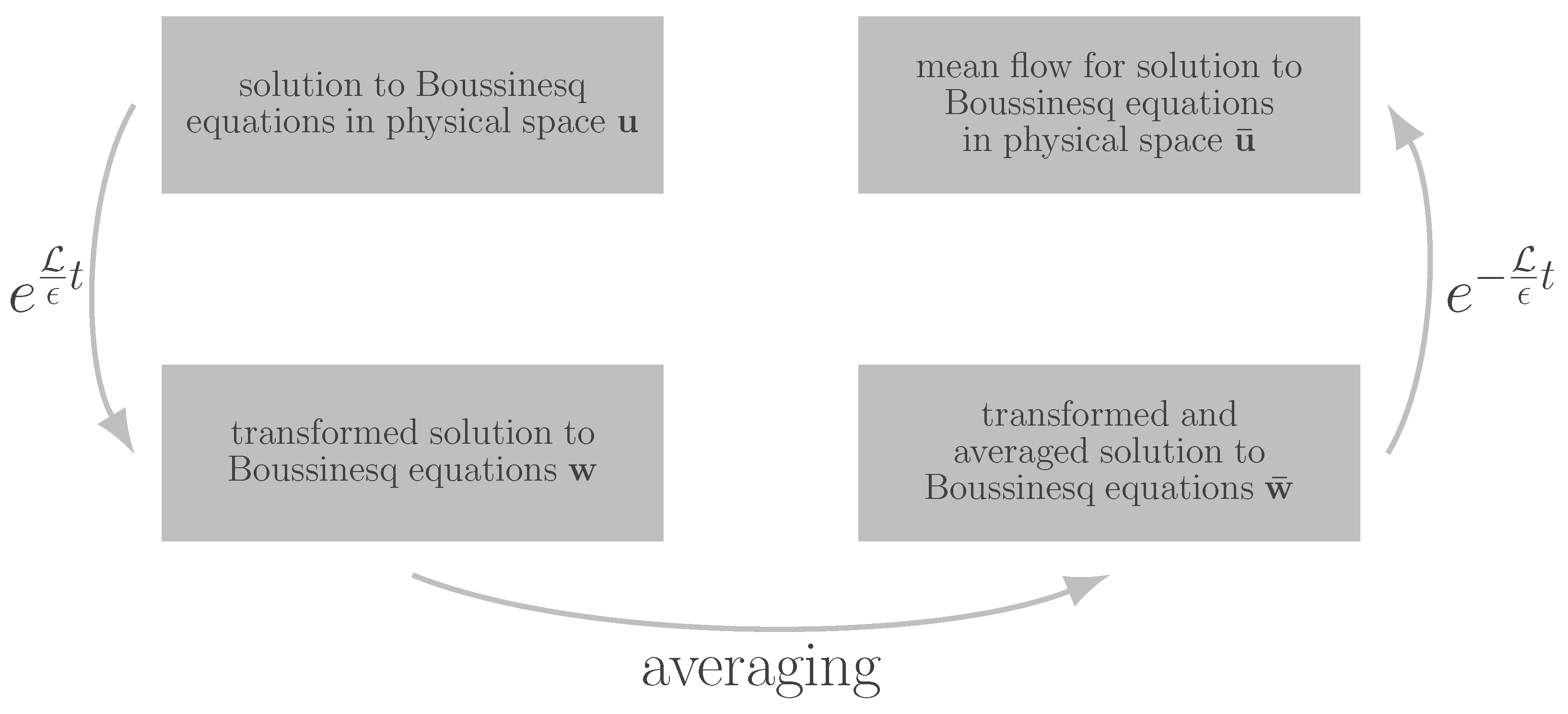
From a fluid dynamics point of view, this type of equations may be interpreted as the mean flow. In the present study, we want to step in a new, less-explored direction by applying the transformation and averaging to a given solution u ( t ) of problem (1) as a diagnostic tool and investigating if such formulations provide a suitable formulation for mean flows. In this case, we evaluate
w ¯ ( t ) = 1 η η / 2 η / 2 K s η w ( t + s ) d s ,
where w is given by Relation (2). The difference between Equations (4) and (5) is that, in the first equation, the averaging procedure is applied to the right-hand side of a differential equation, whereas, in the second equation, it is applied to a given solution of that differential equation. Thus, in the first case, averaging is applied to make a time evolution problem more well-behaved for numerical computations; in the second case, it serves to extract information from data. The averaging is discussed in more detail in Section 2.3.
Already, in [8], it was suggested to use exponential mapping for the formulation of the mean flow for geophysical fluid dynamics applications. However, the approach described there differs from the ideas in the present expositions in the following ways. First, the exponential in this exposition is applied to data representing a solution to the Boussinesq equations. We do not use it to derive analytical expressions for leading order solutions when the method of multiple scales is applied. Second, for the formulation of the mean flow, the authors of [8] proposed to consider only modes which satisfy the condition for resonant triads. In the present exposition, this constraint is relaxed and not only resonant modes, but also other slow modes are admitted for the formulation of the mean flow.
In the present study, the focus is the 2D Boussinesq equations. In particular, we study the case of an initial buoyancy distribution that decays with time:
The Boussinesq equations are
u t + u u x + w u z + x Δ 1 · u · u N ρ z = ν Δ u ,
w t + u w x + w w z + z Δ 1 · u · u N ρ z + N ρ = ν Δ w ,
ρ t + u ρ x + w ρ z N w = κ Δ ρ ,
where the the Brunt–Väisälä frequency is N = b g ρ 0 . We assume periodic boundary conditions with the vector of unknowns u = ( v , ρ ) . The divergence constraint is given by d i v v = 0 , where v = ( u , w ) T . The pressure obeys a Poisson equation (see [24]). We study the averaging technique for oscillating and decaying dynamics.
In [8], the following identity was derived for a leading order solution of the rotating Boussinesq equations:
u 0 = e τ L u ¯ ,
where u ¯ satisfies an averaged equation, which contains the non-linearity and is given by
d u d t = lim τ 1 τ 0 τ e s L B ( e s L u ( t ) , e s L u ( t ) ) d s .
Note that we take τ in Equation (10). The integrand in Equation (10) can be represented using a Fourier decomposition in space. Applying the Riemann–Lebesque lemma, one sees that only the modes which form direct resonances are retained by the intregration process. However, we relax this constraint and allow some slow oscillations too. This provides a new tool to define mean flows, where we allow selected oscillations to be in the formulation. The new averaging procedure, which differs from the one given by Equation (10), is of central significance to decide which oscillations remain in the solution and is explained in more detail in Section 2.3.
In the remainder of the article, we describe the details of the diagnostic we use to compute the time-mean flow. In the results section, we (1) present preliminary numerical results that show the behavior of the mapping and averaging on the time-evolution of the buoyancy, (2) characterize the mean flow that results from the mapping and averaging, including exploring the effect of changing the averaging window, and (3) compute the time rate-of-change of the buoyancy, to assess whether it can mitigate the oscillatory stiffness for use in numerical methods.

2. Methods

We compute a temporal mean flow for solutions to the Boussinesq Equations. For that, the following procedure is pursued. First, a solution to the Boussinesq Equations, denoted as u , is computed. Particulars can be found in Section 2.1. Then, the exponential of the linear operator is applied to the solution and we obtain the mapped solution w . The computation of the exponential is described in Section 2.2 and Appendix A. In the next step, the mapped solution is averaged according to Equation (5). Thus, we compute w ¯ . The mapped solution w can be represented in terms of spatial Fourier modes. When applying the averaging from Equation (5), we can choose, which modes shall be averaged or remain in the solution, by adjusting η , denoted as the averaging window. If the period of a mode is larger than η , the mode will still be present in the solution—see Section 2.3 for details. In the last step, we apply the inverse of the transformation (2).
Performing the previously described procedure, we create several data sets:
  • The unchanged data from the numerical solution of the 2D Boussinesq equations u ;
  • The data after applying the transformation, yielding the mapped solution w ;
  • The data after applying the transformation and the averaging procedure, which give the averaged solution w ¯ ;
  • The data after applying the inverse transformation u ¯ .
The above items are illustrated in Figure 1. Comparison of the data sets helps to assess how well the proposed procedure is suited to describe mean flows and potentially to be used for time-stepping methods.

2.1. Numerical Computation of Solutions to the Boussinesq Equations

We compute numerical solutions using the Dedalus software [25]. We use a Fourier discretization in space in a 2 π periodic 2D domain and 3rd-order 4-stage Runge–Kutta Method (RK433) time-stepper. For all the simulations, the time step is Δ t = 0.001, the spatial grid is ( N x , N z ) with N x = N z = 128 , the viscosity is ν = 0.0001, and the dissipation for buoyancy is κ = 0.0001. For the initial condition, u ( 0 , x ) = w ( 0 , x ) = 0 , while the initial buoyancy is
ρ ( 0 , x ) = ϵ f sin ( 3 z ) sin ( 3 x ) ,
with ϵ f = 25 . The energy oscillates between kinetic and potential energy in time while it decays. The higher the value of N, the more frequent the oscillations. Figure 2 shows an example of the dynamics in decay as it oscillates between kinetic and potential energy. At some time after the simulation begins, higher frequency oscillations are excited, providing a challenge for studying oscillatory mean flows.
In this study, we use 3 different values of N: N = 1 , 10 , and 20. We define the Froude number to be a function of the character of the initial condition, using similar ideas to [12], who studied the forced case
F r = 2 ( ϵ f k f 2 ) 1 3 N ,
which gives us equivalent Froude numbers of F r = 10.6 , 1.06 , and 0.53.

2.2. Fourier Analysis and the Computation of the Exponential of L with the Divergence Constraint

For the implementation of the exponential of the linear operator, we apply a Fourier expansion in space to the solutions of the Boussinesq equations, i.e., we have
u ( t , x ) = k = N N u ^ ( t ) e i k · x .
Each mode e i k · x is applied to the linear operator, which is given by
L u = x Δ 1 N ρ z z Δ 1 N ρ + N ρ N w .
Consequently, a 3 × 3 matrix is obtained for each mode. Then, the matrix exponentials for the different modes are computed. To compute the exponential of the linear operator, it is sufficient to know the exponential for each mode e i k · x . Due to linearity, we have
e L ϵ t u ( t , x ) = k = N N e L ϵ t e i k · x u ^ ( t ) = k = N N B k u ^ ( t ) e i k · x ,
where B k e i k · x = e L ϵ t e i k · x . Applying the exponential, we obtain w , given by (2).
Here, we briefly describe the computation of the matrix exponential. Further details of the computations can be found in Appendix A. The horizontal wave number is denoted as k 1 . With k 3 , we refer to the vertical wave number. First, the eigenvalues are computed. Then, the corresponding eigenvectors are identified. With the eigenvectors, we know the transformation matrix T k and can also compute its inverse T k 1 . In the computations, we distinguish between four different cases (first: k 1 = 0 , k 3 = 0 ; second: k 1 = 0 , k 3 0 ; third: k 1 0 , k 3 = 0 ; fourth: k 1 0 , k 3 0 ). The matrices are diagonalizable, except for the case k 1 = 0 , k 3 0 . For that case, we compute the Jordan normal form. To compute the exponential of the matrix B k , where B k comes from the spatial discretization of the linear operator and depends on the wave numbers, we use the identity exp ( B k ) = T k exp ( M k ) T k 1 . In the relation, the matrix M k is the diagonal matrix or the matrix in Jordan normal form with the computed eigenvalues. Finally, we enforce the divergence constraint.

2.3. Averaging with a Convolution Integral

A transformed solution of the Boussinesq equations w is convolved by applying a scaled filter function K :
K s η = 1 K 0 exp 1 ( s / η 1 / 2 ) ( s / η + 1 / 2 ) ,
where the constant K 0 is chosen so that integrating the kernal function along the real line gives 1. We scale the filter function by choosing an averaging window η . The idea behind the choice of the averaging window η is that it must mitigate the fast oscillations while leaving the coarser behavior of the solution unaffected. The bigger the averaging window, the more oscillations are mitigated. The smaller the averaging window, the more oscillations are resolved. Temporal averaging was also investigated in other contexts, like ordinary differential equations [1], heterogeneous multiscale methods [26,27], and PDE analysis [8].
To further illustrate the averaging, let us suppose that a slow function is superimposed by a fast periodic function with zero mean. When we compute the integral of the fast function over an interval of length η , assuming that η is as large as a few times the period of the fast periodic function, the positive and negative contributions cancel each other. However, the integrand is weighted by the scaled kernel function K with compact support, which decays fast close to the boundary of the compact support. In addition, we do not assume that the length of the exact period is known. Thus, in the general case, the oscillations are not exactly canceled, but rather they are mitigated, as can be seen in Figure 3. Technical details of the averaging can be found in [27] in Lemma 2.2.

3. Results and Discussion

We begin with a description of the time evolution of the dynamics (unaveraged) for the specific case studied in this work. In all cases, the initial condition is given by (11) and the velocity components are zero initially.
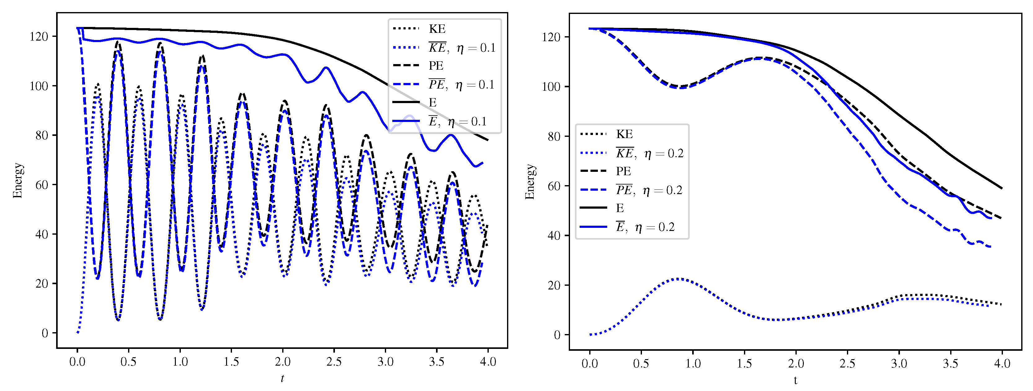
Figure 2 shows the evolution of total, potential, and kinetic energy for N = 10 on the left and N = 1 on the right. The data are shown in black lines for the unaveraged case with total energy: solid, kinetic energy: dotted, and potential energy: dashed. These graphs show that the dynamics decay as it evolves, and that the case with the larger Brunt–Väisälä frequency has more frequent energy exchanges between potential and kinetic energy compared to the N = 1 case.
These more frequent energy exchanges in potential and kinetic energy can also be seen by examining the time history of u [ 3 ] ( x p , z p , t ) = ρ ( x p , z p , t ) at a single, randomly chosen point ( x p , z p ) = ( 2 π 60 128 , 2 π 60 128 ) . Other choices of the location of the point show similar results. This will be explored in the next section where we examine vertical slices, which show the time evolution for all the values of z at a fixed x p . Compare the solid black line in the upper right panel of Figure 4 for N = 10 to the same style of line in Figure 4 for the N = 1 data. For the N = 10 case, the solution has more frequent oscillations than the N = 1 case. For both values of N, the solution breaks up into higher oscillations as the solution decays. This feature is used to illustrate the effect of the averaging in the following sections.
Finally, before we go on to study the effect of the averaging, we look at the time evolution of the single point data in the mapped domain w [ 3 ] ( x p , z p , t ) . These data are computed by applying the matrix exponential, as in (2), to the vector u . This has the effect of showing what the time evolution of the solution looks like in the moving frame and allows us to observe the effect of the ‘phase scrambling’ in the nonlinear term, as in (3). The evolution in the moving frame is shown in the solid black line in the left panels of Figure 4. For N = 20 and N = 10 , there are more frequent oscillations in the moving frame than in the ordinary frame shown in the right panel. In contrast, for the N = 1 case, the difference between the solution in the moving frame w and the ordinary frame u is not as different as the other cases, which is because the moving frame is slow for N = 1 .
In the next three subsections, we examine the effect of the mapping and averaging on these oscillatory, decaying solutions.

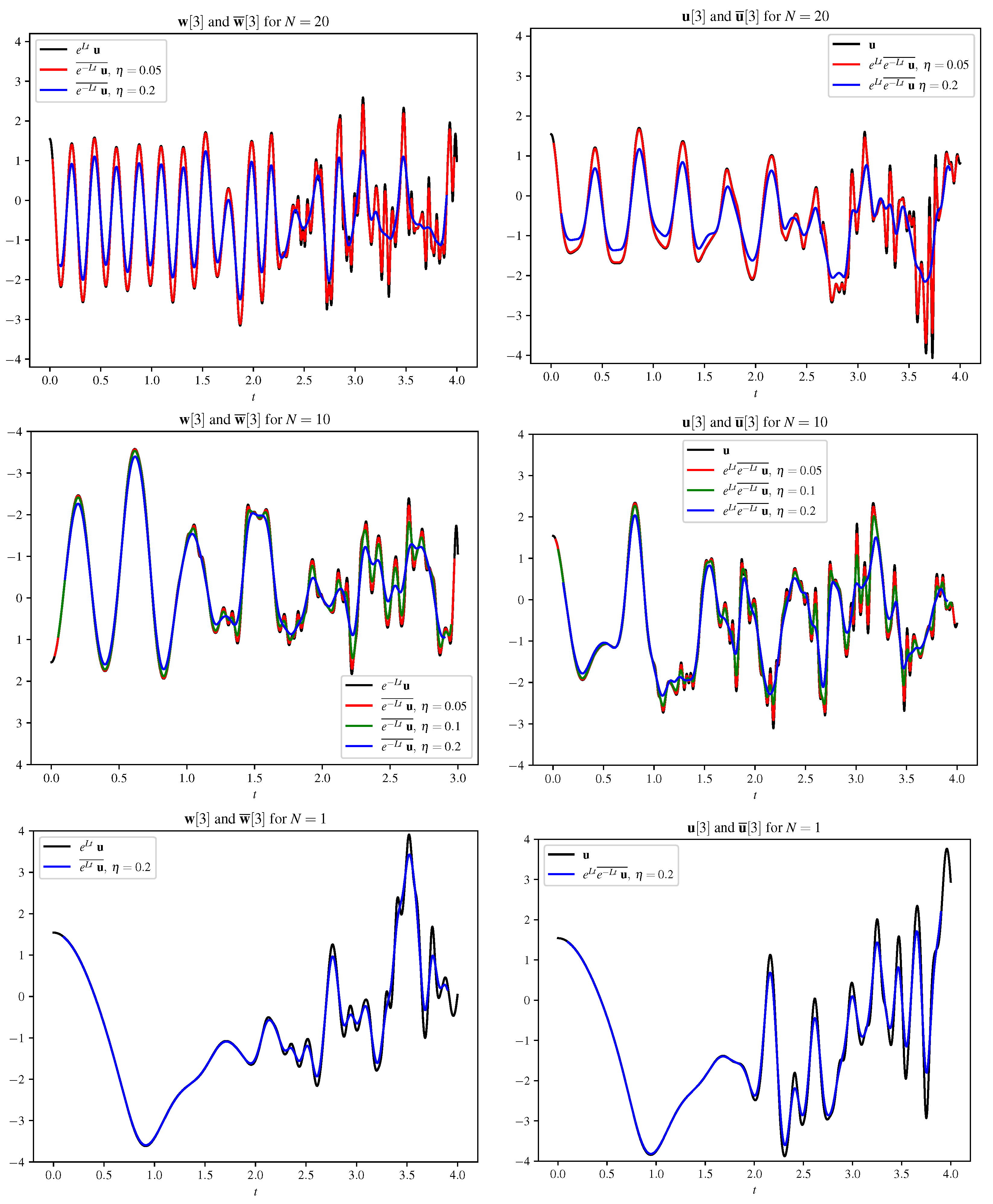
3.1. Impact of Mapping and Averaging

We now describe the impact of the mapping and averaging technique on the time evolution of the ρ dynamics by examining time series for three different values of N in the context of the four data sets ( u , w , w ¯ , u ¯ ) described in the second paragraph of Section 2. Because we focus on ρ , when u , w , w ¯ , u ¯ appear in a figure, these are the third component of the vector field.
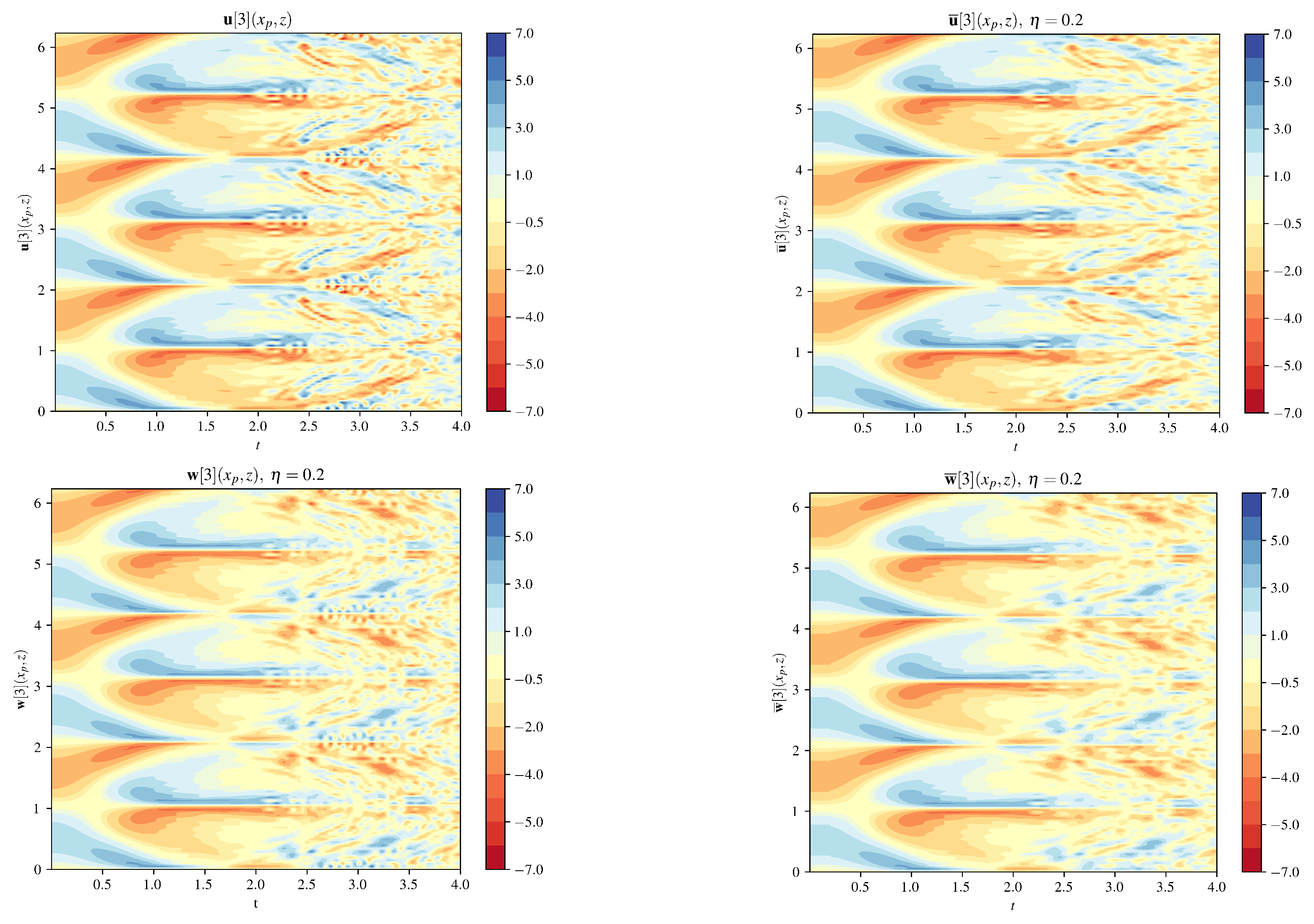
Figure 4 presents the time series at a single point, with each row of the figure corresponding to a different value of N. In all three rows, the left panel shows the time evolution in the moving frame w and its average w ¯ . In contrast, the right panel shows the ordinary variable u and the average in the moving frame mapped back to the ordinary frame u ¯ . The significance of the left panels is that they show the result of how the oscillations are being ‘scrambled’ and evolved by the nonlinear term in (2) as the solution undergoes decay from its initial condition. A first observation is that, for the two higher values of N studied, the oscillations in w , the moving frame variables, are faster than those observed in u . For some parameter regimes in 2D Boussinesq dynamics, one might expect the dynamics of w to be of lower frequency than u , not higher, so further studies of the case with forcing, where low frequency buoyancy layers are formed, could be interesting (see [12]).
A second observation is that, for the higher values of N at later times, when the faster oscillations appear, the averaging from the nonlinear phase scrambler in the moving frame, w ¯ , tracks the mean value, as expected. This is in contrast to the panel on the right where, for example, for N = 20 in the range 3.5 < t < 4 , when the average is mapped back to the ordinary frame, the average does not track the mean value. This is also as expected because, in this domain, the average is modulated by the oscillations. As mentioned in the introduction, ref. [1] gives an example of why straightforward time averages, in the unmapped equations, do not give accurate results. The comparison that we just described, where the modulated mean, u ¯ , does not necessarily track the mean of u , is a characteristic feature of averages taken in the modulated domain. We discuss this more in the next section where we consider the mean-flow possibilities.
Finally, we make a few observations about the effect of the averaging window η on the mean of the time series. In Figure 4, on the left panels, the effect of varying the averaging window is shown. The longer the averaging window, the more the amplitudes are damped. At early times, for N = 20 , the main effect is to reduce the magnitude of the oscillations, but, at later times, the red line, for which a small averaging window η = 0.05 was used, shows little difference from the unaveraged case. However, when the largest averaging window is applied, for η = 0.2, the blue line for 3 < t < 4 shows that the mapping and averaging tracks the mean of the oscillations. This similar behavior can be seen in the unmapped domain on the right, where, as pointed out earlier, the blue line, with the larger averaging window, is slower, but does not follow the mean of the oscillations. For the middle panel, when N = 10 , we show three different averaging window lengths ( η = 0.05, 0.1, and 0.2). For the largest averaging window (blue line), the mean tracks the mean of the oscillations. This is true in the right panel as well. Finally, for the lowest value of N, N = 1 , the choice of averaging window has a similar effect, except that, at early times, it does not have that much of an effect, while, at later times, when the faster oscillations begin, it appears to track through the mean value.
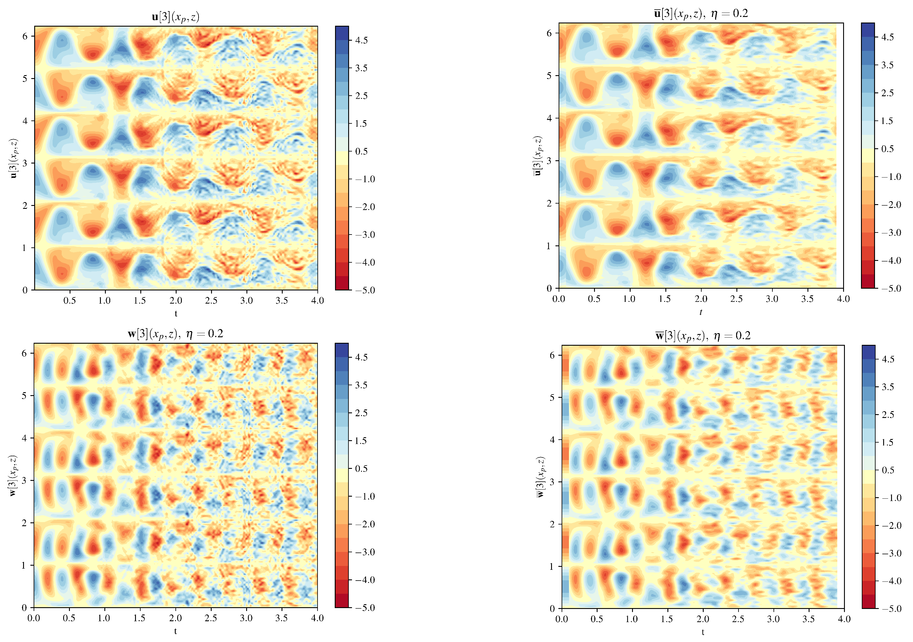
Figure 5 and Figure 6 show the time evolution of four data sets for every point in the z plane for a fixed x = x p , for N = 10 and N = 1 , respectively. Rather than grouping w and w ¯ together and u and u ¯ together, as in the previous paragraphs, this time we show a panel for each data set in the same counterclockwise order as shown in Figure 1. The upper left graph shows the time evolution of u , the lower left shows the time evolution in the moving frame w , and the lower right panel shows the average in the moving frame w ¯ . For N = 10 , u oscillates between positive and negative values of the buoyancy and then we see the creation of higher frequency waves as the solution decays. We observe that, even when the higher frequency oscillations appear, larger scale (in time) patterns can also be seen. The lower right panel shows the effect of averaging in the moving frame, where the larger structures in time now look smoother. For the case when N = 1 , the oscillatory pattern between positive and negative values are less frequent, since N is smaller. Comparing the two cases N = 10 and N = 1 , the graphs show that N = 1 has an overall large-scale (in time) pattern of oscillations, whereas the N = 10 case has frequent temporal oscillations.
Finally, we examine the effect of the mapping and averaging on the energy. Figure 2 shows the effect of the averaging on the kinetic, potential, and total energy for the u and u ¯ data sets for N = 10 on the left and N = 1 on the right. For N = 10 , the mean tracks the oscillation between kinetic and potential, and shows an oscillation in the overall mean flow, which is discussed a bit more in the next section. For N = 1 , the mean total energy decays faster than total energy, due to the average over the oscillations.

3.2. Definition of a Mean Flow

For a preliminary assessment of whether the mapping and averaging procedure could be a suitable definition of a mean flow for the 2D Boussinesq equations, we break the unknowns into its mean and fluctuation:
u = u ¯ + u ,
and in the moving frame:
w = w ¯ + w .
Integration over the oscillations would give us zero as positive and negative components cancel each other. From a mean flow, we would expect that only the mean behavior without the departures is retained.
Revisiting Figure 4, we make the following two observations: (1) The fastest variations in the solution are not visible anymore; (2) The amplitudes are damped when the solutions have steep gradients. Therefore, the component which is not retained contains fast oscillations and has positive and negative components.
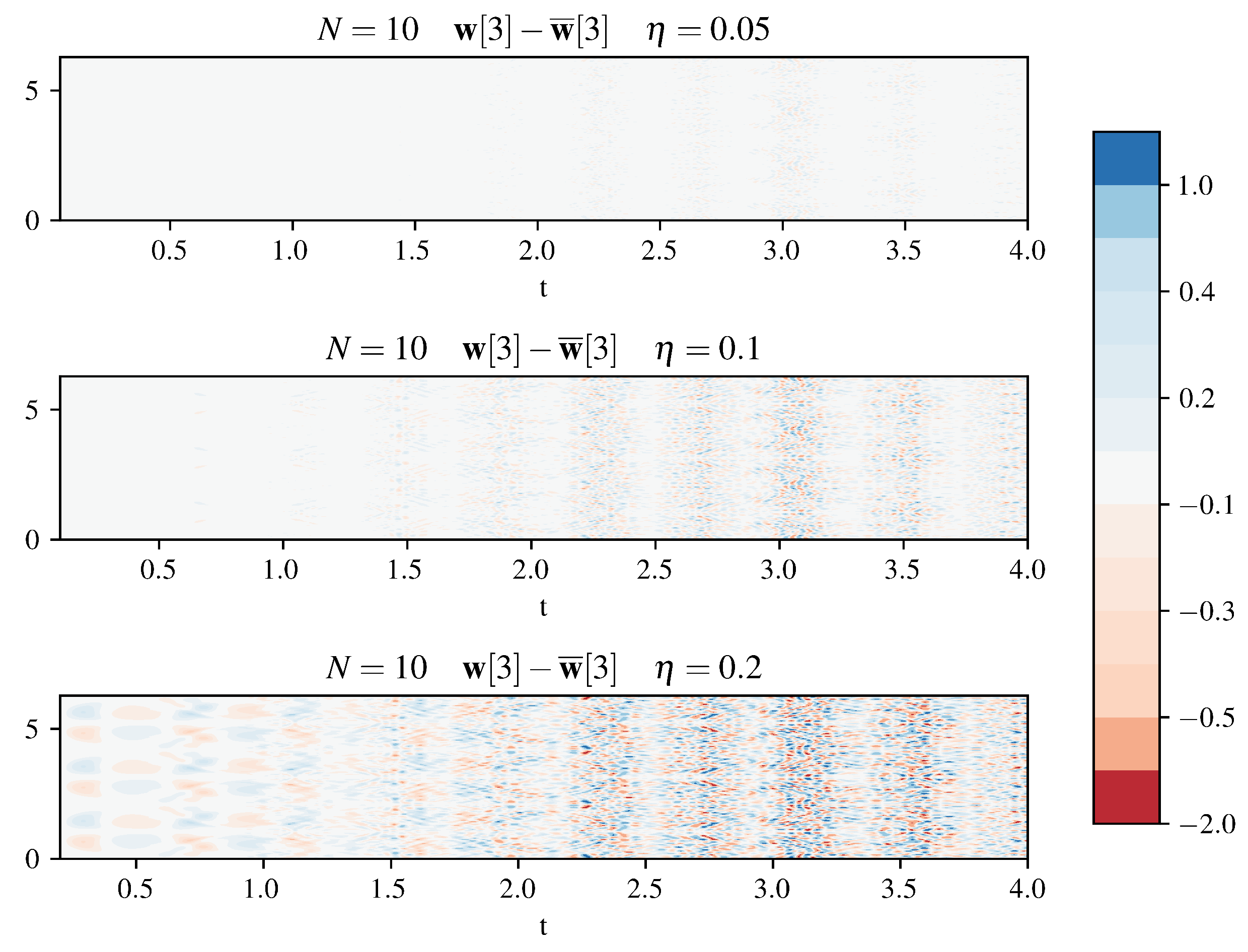
Figure 7 shows the point-wise departure from the mean in the moving frame, w , for three different averaging windows. The main variations from the mean occurs when the filtering window is larger, as we expect, and also where there are higher oscillations at later times in the simulation. We also observe that, once the higher frequency oscillations have begun, the variation from the mean is also nearly periodic. Variation from the mean for the ordinary frame u (not shown) shows a different detailed pattern with a similar periodicity.
Additionally, the choice of the averaging window allows us to determine which oscillations should be filtered and how strong the damping should be. For large averaging windows, more oscillations are filtered and the damping is stronger than for small averaging windows. This means that the definitions of the mean flow and the departures from the mean depend on the choice of the length of the averaging window. In both the moving frame and the ordinary frame, periodic patterns can be seen in the deviation from the mean.
Finally, we point out that total energy in Figure 2 for N = 10 shows an oscillation in the mean and that the the distance from the mean to the instantaneous energy decay is the energy from the variations from the mean. This oscillatory pattern in the mean flow is a potential area to explore in further work.
Our observation in the last section, that the mapping and averaging tracks the mean in the moving frame but not in the ordinary frame, will also be interesting in the context of fast singular limits, where it is expected that low-frequency structures will appear over time, rather than only high frequencies. To obtain a more complete understanding a wider range of behaviors, such as the creation of low frequencies, would be useful.

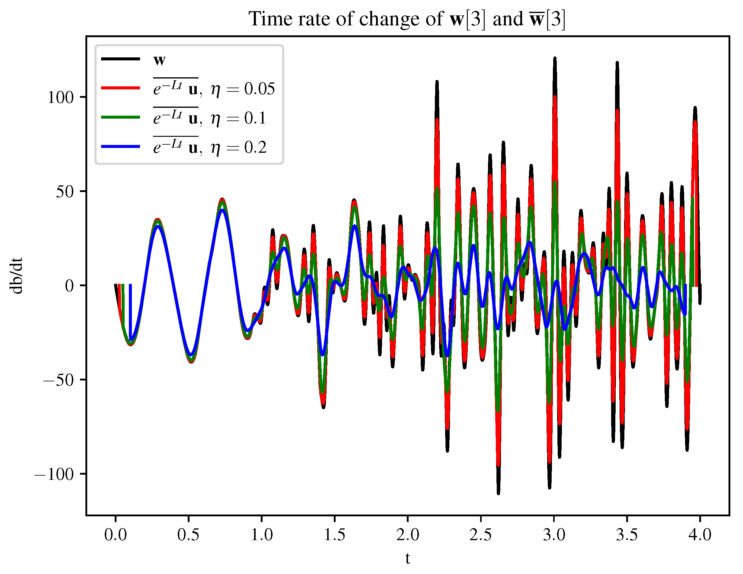
3.3. Potential for Use in Numerical Methods

As mentioned in the introduction, the technique explored in this paper has been proposed for use as a prediction step for time-parallel predictor–corrector methods used to solve PDEs of type (1). An error bound for a predictor-step algorithm using this method can be found in [22] and does not require that ϵ be small. As a part of the error estimate, the error bound for the approximation of the time rate of change of the unknowns depends on the averaging window, η . We therefore are interested in whether the time rate of change of the variable examined in this paper has this property. To study this, we apply a first-order finite difference method to the moving frame w and w ¯ data sets. Figure 8 shows the time rate of change for the N = 10 case depicted in the time series of Figure 4. This shows that the nonlinear averaging process reduces the amplitude and frequency of the oscillations, making it possible that this method could provide a good predictor for numerical methods. However, it is clear that the filter width matters, in line with the error estimate, and that it may need to be dynamically adjusted. For example, the solid blue line in Figure 8 shows that it has fewer large oscillations than the unaveraged case, but whether this is adequate to take larger time steps is unclear.
We have also pointed out, in previous sections, that, for the simulations in this study, the actual mean tracks w ¯ rather than u ¯ . It would be of interest to explore this more fully in future work.

4. Conclusions

In this work, we have presented numerical studies of the oscillating and decaying 2D Bousinnesq equations and developed a diagnostics to study a nonlinear averaging procedure. The goal was to present a preliminary study of the impact of the mapping and averaging technique by using it as a diagnostic, then assess whether it could make a good definition of a mean flow and potentially help mitigate oscillatory stiffness in numerical methods.
We made the following observations:
  • The nonlinear averaging procedure depends strongly on the value of η , but could potentially provide a reasonable representation of the time-mean of the solutions, whether or not N is large. Further, the average ‘modulates’ the waves, as in (2). This has the effect that the mean u ¯ depends on how fast the oscillations are in the exponential operator (2), which could be interesting for further studies. Further work is needed to assess whether this would be a good definition of a mean flow in fluid dynamics. For example, it would be interesting to examine a case that admits a low-frequency solution such as the 2D Boussinesq equations with forcing, as in [12] and examples shown in [8];
  • We also observed that the method could potentially be used to take larger time steps, as has been shown in simple examples [21], and that the ability to do so critically depends on the value of η .

Author Contributions

Conceptualization, B.A.W., T.H. and J.R.; methodology, B.A.W., T.H. and J.R.; software, B.A.W. and J.R.; validation, B.A.W. and J.R.; writing—original draft preparation, B.A.W. and J.R.; writing—review and editing, B.A.W. and J.R.; funding acquisition, B.A.W., T.H. and J.R. All authors have read and agreed to the published version of the manuscript.

Funding

Beth Wingate’s research was funded by the UK Engineering Physical Science Research Council (EPSRC) grant number EP/R029628/1, Leverhulme Trust Research Fellowship RF-2022-013. Juliane Rosemeier’s research was funded by the Deutsche Forschungsgemeinschaft (DFG, German Research Foundation)—463179503. Terry Haut’s research was funded by the US Department of Energy.

Institutional Review Board Statement

Not applicable.

Informed Consent Statement

Not applicable.

Data Availability Statement

Not applicable.

Acknowledgments

We thank the University of Exeter for hosting Juliane Rosemeier’s DFG Walter Benjamin Fellowship, and the US Department of Energy Lawrence Livermore National Laboratory for hosting Juliane Rosemeier and Beth Wingate as visitors.

Conflicts of Interest

The funders had no role in the design of the study; in the collection, analyses, or interpretation of data; in the writing of the manuscript; or in the decision to publish the results.

Abbreviations

The following abbreviations are used in this manuscript:
PDEpartial differential equation
ODEordinary differential equation

Appendix A. Computational Details for the Exponential

Appendix A.1. The Eigenvalues and Eigenvectors

First case:  k 1 = 0 , k 3 = 0 ,
eigenvalues: ω 1 = 0 , ω 2 = i N , ω 3 = i N
eigenvectors: v 1 = 1 0 0 v 2 = 1 2 0 i 1 v 3 = 1 2 0 i 1
Second case:  k 1 = 0 , k 3 0 ,
eigenvalues: ω 1 = ω 2 = ω 3 = 0
eigenvectors: v 1 = 1 0 0 v 2 = 0 0 1
generalized eigenvector: v ˜ = 0 1 N 0
Third case:  k 1 0 , k 3 = 0 ,
In this case, we have the same eigenvalues and eigenvectors as in the the first case.
Fourth case:  k 1 0 , k 3 0 ,
eigenvalues: ω 1 = 0 , ω 2 = i N | k 1 | / k , ω 3 = i N | k 1 | / k
eigenvectors: v 1 = 1 0 0 v 2 = 1 2 i k 1 k 3 | k 1 | k i | k 1 | k 1 v 3 = 1 2 i k 1 k 3 | k 1 | k i | k 1 | k 1

Appendix A.2. Diagonal Matrix or Jordan Normal Form

First case:  k 1 = 0 , k 3 = 0 ,
D = 0 0 0 0 i N 0 0 0 i N
Second case:  k 1 = 0 , k 3 0 ,
J = 0 0 0 0 0 1 0 0 0
Third case:  k 1 0 , k 3 = 0 ,
In this case, we have the diagonal matrix as in the the first case.
Fourth case:  k 1 0 , k 3 0 ,
D = 0 0 0 0 i N | k 1 | k 0 0 0 i N | k 1 | k

Appendix A.3. Transformation Matrix and Inverse

First case:  k 1 = 0 , k 3 = 0 ,
T = 1 0 0 0 i 2 i 2 0 1 2 1 2 , T 1 = 1 0 0 0 i 2 1 2 0 i 2 1 2
Second case:  k 1 = 0 , k 3 0 ,
T = 1 0 0 0 0 1 N 0 1 0 , T 1 = 1 0 0 0 0 1 0 N 0
Third case:  k 1 0 , k 3 = 0 ,
The transformation matrix and inverse are the same as in the the first case.
Fourth case:  k 1 0 , k 3 0 ,
T = 1 i 2 k 1 k 3 | k 1 | k i 2 k 1 k 3 | k 1 | k 0 i 2 k 1 k i 2 k 1 k 0 1 2 1 2 , T 1 = i k k 1 i k 1 k i k 1 k 3 | k 1 | k 0 0 1 2 i 2 k 1 k 0 1 2 i 2 k 1 k

Appendix A.4. The Matrices with Divergence Constraint

First case:  k 1 = 0 , k 3 = 0 ,
1 0 0 0 1 2 e i N t + e i N t 1 2 e i N t e i N t 0 1 2 e i N t + e i N t 1 2 e i N t + e i N t
Second case:  k 1 = 0 , k 3 0 ,
0 0 0 0 1 2 e i N t + e i N t 1 2 e i N t e i N t 0 1 2 e i N t + e i N t 1 2 e i N t + e i N t
Third case:  k 1 0 , k 3 = 0 ,
1 0 0 0 0 0 0 0 1
Fourth case:  k 1 0 , k 3 0 ,
0 k 3 2 k 1 e i N k 1 | k | t + e i N k 1 | k | t i k 3 | k 1 | 2 | k | k 1 e i N k 1 | k | t + e i N k 1 | k | t 0 1 2 e i N k 1 | k | t + e i N k 1 | k | t i | k 1 | 2 | k | e i N k 1 | k | t + e i N k 1 | k | t 0 i k 2 k 1 e i N k 1 | k | t e i N k 1 | k | t 1 2 e i N k 1 | k | t + e i N k 1 | k | t

References

  1. Verhulst, S.F.; Murdock, J. Averaging Methods in Nonlinear Dynamical Systems, 2nd ed.; Springer: New York, NY, USA, 2007. [Google Scholar] [CrossRef]
  2. Herring, J.R. Approach of axisymmetric turbulence to isotropy. Phys. Fluids 1974, 17, 859–872. [Google Scholar] [CrossRef]
  3. Herring, J.R.; Métais, O. Numerical experiments in forced stably stratified turbulence. J. Fluid Mech. 1989, 202, 97–115. [Google Scholar] [CrossRef]
  4. Métais, O.; Herring, J.R. Numerical simulations of freely evolving turbulence in stably stratified fluids. J. Fluid Mech. 1989, 202, 117–148. [Google Scholar] [CrossRef]
  5. Babin, A.; Mahalov, A.; Nicolaenko, B. Global splitting, integrability and regularity of 3D Euler and Navier-Stokes equations for uniformly rotating fluids. Eur. J. Mech. B Fluids 1996, 15, 291–300. [Google Scholar]
  6. Babin, A.; Mahalov, A.; Nicolaenko, B.; Zho, Y. On the asymptotic regimes and the strongly stratified limit of rotating Boussinesq equations. Theor. Comput. Fluid Dyn. 1997, 9, 223–251. [Google Scholar] [CrossRef]
  7. Bogoliubov, N.; Mitropolsky, Y. Asymptotic Methods in the Theory of Nonlinear Oscillations; Gordon and Breach: New York, NY, USA, 1961. [Google Scholar]
  8. Embid, F.; Majda, J. Averaging over fast gravity waves for geophysical flows with arbitrary potential vorticity. Commun. Partial. Differ. Equ. 1996, 21, 619–658. [Google Scholar] [CrossRef]
  9. Klainerman, S.; Majda, A.J. Singular limits of quasilinear hyperbolic systems with large parameters and the incompressible limit of compressible fluids. Commun. Pure Appl. Math. 1981, 34, 481–524. [Google Scholar] [CrossRef]
  10. Schochet, S. Fast Singular Limits of Hyperbolic PDEs. J. Differ. Equ. 1994, 114, 476–512. [Google Scholar] [CrossRef]
  11. Newell, A. Rossby wave packet interactions. J. Fluid Mech. 1969, 35, 255–271. [Google Scholar] [CrossRef]
  12. Smith, L.M. Numerical study of two-dimensional stratified turbulence. Contemp. Math. 2001, 283, 91–106. [Google Scholar]
  13. Smith, L.; Waleffe, F. Generation of slow large scales in forced rotating stratified turbulence. J. Fluid Mech. 2002, 451, 145–168. [Google Scholar] [CrossRef]
  14. Kafiabad, H.A.; Vanneste, J.; Young, W.R. Wave-averaged balance: A simple example. J. Fluid Mech. 2021, 911, R1. [Google Scholar]
  15. Wagner, G.L.; Young, W.R. Available potential vorticity and wave-averaged quasi-geostrophic flow. J. Fluid Mech. 2015, 785, 401–424. [Google Scholar]
  16. Yamazaki, H.; Cotter, C.; Wingate, B. Time parallel integration and phase averaging for the nonlinear shallow water equations on the sphere. Q. J. R. Meteorol. Soc. 2023. accepted. [Google Scholar] [CrossRef]
  17. Majda, A.; Embid, P. Averaging over Fast Gravity Waves for Geophysical Flows with Unbalanced Initial Data. Theoret. Comput. Fluid Dyn. 1998, 11, 155–169. [Google Scholar] [CrossRef]
  18. Whitehead, J.P.; Haut, T.; Wingate, B. The effect of two distinct fast time scales in the rotating, stratified Boussinesq equations: Variations from quasi-geostrophy. Theor. Comput. Fluid Dyn. 2018, 32, 713–732. [Google Scholar] [CrossRef]
  19. Mu, P.; Ju, Q. Three-scale singular limits of the rotating stratified Boussinesq equations. Appl. Anal. 2021, 100, 2405–2417. [Google Scholar] [CrossRef]
  20. Jones, D.A.; Mahalov, A.; Nicolaenko, B. A Numerical Study of an Operator Splitting Method for Rotating Flows with Large Ageostrophic Initial Data. Theor. Comput. Fluid Dyn. 1999, 13, 143. [Google Scholar] [CrossRef]
  21. Haut, T.; Wingate, B. An asymptotic parallel-in-time method for highly oscillatory pdes. SIAM J. Sci. Comput. 2014, 36, A693–A713. [Google Scholar] [CrossRef]
  22. Peddle, A.G.; Haut, T.; Wingate, B. Parareal convergence for oscillatory pdes with finite time-scale separation. SIAM J. On Scientific Comput. 2019, 41, A3476–A3497. [Google Scholar] [CrossRef]
  23. Rosemeier, J.; Haut, T.; Wingate, B. Multi-level Parareal algorithm with Averaging for Oscillatory Problems. SIAM J. Sci. Comput. 2023. submitted. [Google Scholar]
  24. Majda, A. Introduction to P.D.E.’s and Waves for the Atmosphere and Ocean; Courant Lecture Notes; New York University, Courant Institute of Mathematical Sciences and American Mathematical Society: New York, NY, USA, 2002; Volume 9. [Google Scholar]
  25. Burns, K.J.; Vasil, G.M.; Oishi, J.S.; Lecoanet, D.; Brown, B.P. Dedalus: A Flexible Framework for Numerical Simulations with Spectral Methods. Phys. Rev. Res. 2020, 2, 023068. [Google Scholar] [CrossRef]
  26. Weinan, E.; Engquist, B. Multiscale modeling and computation. Not. Am. Math. Soc. 2003, 50, 1062–1070. [Google Scholar]
  27. Engquist, B.; Tsai, R. Heterogeneous multiscale methods for stiff ordinary differential equations. Math. Comput. 2005, 74, 1707–1742. [Google Scholar] [CrossRef]
Figure 1. The figure illustrates how the data sets for the mean flow representation are created. The gray boxes represent the data sets. The arrows show the operations which are applied to the data sets.
Atmosphere 14 01523 g001
Figure 2. The total, kinetic, and potential energy (black lines) compared to their mean values (blue lines). The panel on the left shows the case for N = 10 and η = 0.1. The panel on the right shows the case for less frequent oscillations when N = 1 and η = 0.2. Solid lines are the total energy, dotted lines are the kinetic energy, and dashed lines are the potential energy. The solutions oscillate between kinetic and potential energy as they decay. The principal effect of the averaging window on the mapped and averaged solution is to track the frequency of the energetic exchanges between kinetic and potential energy and to reduce the magnitude of the oscillations. The case N = 10 on the left suggests that the phase-averaged mean flow shows an oscillatory total energy.
Atmosphere 14 01523 g002
Figure 3. This figure demonstrates the effect of the averaging window on oscillatory functions. In the left panel, the averaging window η is smaller than the period of the oscillations. The data are barely altered. In the right panel, the averaging window η is larger than the period of the oscillations. Therefore, the oscillations are damped and the mean value is between the peaks and valleys of the signal.
Atmosphere 14 01523 g003
Figure 4. Time series at a single point for the 3rd component of each vector field. The top row is for N = 20 , middle for N = 10 , and bottom for N = 1 . Panels on the left show the time evolution of the data in the moving frame, while, on the right, they depict the evolution in the ordinary frame. Within each graph, colored lines showing the effect of changing the averaging window. As N decreases, there is less difference between the dynamics in the moving frame and the ordinary frame, an effect of the moving frame oscillating at a slower rate over the time scale of the simulation. There are more oscillations in the moving frame, where the averaging takes place, than in the ordinary frame.
Atmosphere 14 01523 g004
Figure 5. Time evolution of the 3rd component of the 4 data sets described in Figure 1 for N = 10 . The top left panel shows u in the ordinary frame. The oscillatory pattern here is also seen in the potential energy shown in Figure 2. The large-scale pattern of oscillations between positive and negative values can be seen even as higher frequency waves appear. There are approximately 2 times more oscillations in w than in the ordinary domain. The appearance of the waves is more noticeable starting at approximately t = 1 . The lower right panel shows the time evolution of the average in the moving frame w ¯ , which smooths the higher frequency oscillations. Finally, mapping back to the ordinary frame, the upper right panel shows the result of the mapping and averaging on the variables in the ordinary frame, u ¯ .
Atmosphere 14 01523 g005
Figure 6. Time evolution of the 3rd component of the 4 data sets described in Figure 1 for N = 1 . The difference between the ordinary frame (top left panel) and mapped frame (bottom left frame) is less pronounced than the corresponding frames for N = 10 (Figure 5) because the oscillations in the exponential operator for N = 1 are less frequent. The higher frequencies that appear later in the simulation are smoothed by the averaging, with the result in the top right panel, which shows the result of the mapping and averaging in the ordinary domain u ¯ .
Atmosphere 14 01523 g006
Figure 7. This figure shows the departure from the mean for three different averaging windows, η , for the case when N = 10 , in the moving frame. As the averaging window, η , is increased, the excursions from the mean flow also increase. The excursions also show a periodic pattern.
Atmosphere 14 01523 g007
Figure 8. This figure shows the time rate of change of the 3rd component of w and w ¯ . The wider the value of η , the smaller the amplitude of the time rate of change, and, in some cases, the less frequent the oscillations. While this could be useful for taking large time steps, the degree of regularity depends strongly on the value of η .
Atmosphere 14 01523 g008
Disclaimer/Publisher’s Note: The statements, opinions and data contained in all publications are solely those of the individual author(s) and contributor(s) and not of MDPI and/or the editor(s). MDPI and/or the editor(s) disclaim responsibility for any injury to people or property resulting from any ideas, methods, instructions or products referred to in the content.

