Article

Flash Drought and Its Characteristics in Northeastern South America during 2004–2022 Using Satellite-Based Products

by
Humberto Alves Barbosa
Laboratório de Análise e Processamento de Imagens de Satélites (LAPIS), Instituto de Ciências Atmosféricas, A. C. Simões Campus, Universidade Federal de Alagoas, Maceió 57072-900, Brazil
Atmosphere 2023, 14(11), 1629; https://doi.org/10.3390/atmos14111629
Submission received: 5 September 2023 / Revised: 27 October 2023 / Accepted: 27 October 2023 / Published: 30 October 2023
(This article belongs to the Special Issue Climate Variability and Change in Brazil)

Abstract

:
The term flash drought describes a special category of drought with rapid onset and strong intensity over the course of days or weeks. To characterize the impact of flash droughts on vegetation coverage, this study assessed the influence of soil water deficits on vegetation dynamics in the northeastern South America region by combining time series of vegetation index, rainfall, and soil moisture based on satellite products at a daily time scale. An 18-year analysis, from 2004 to 2022, of the Normalized Difference Vegetation Index (NDVI), Standard Precipitation Index (SPI), and surface soil moisture (SSM) was performed based on three different satellite remote sensing estimates: the spinning enhanced visible and infrared imager (SEVIRI) and the integrated multi-satellite retrievals algorithm (IMERG), and the soil moisture and ocean salinity (SMOS). The results revealed that flash drought events exerted dramatic impacts on terrestrial ecosystems in the study region during the first two decades of the 2000s, with changes in seasonal and regional vegetation dynamics. Further, the fixed-threshold values to characterize flash drought events were suggested as the timing when the water deficit was less than −1.0 units and vegetation index reached the value equal to +0.3 during five consecutive weeks or more, coupled with soil moisture rates below 40% percentile, leading to a strong region-wide drought throughout the entire region. Additionally, the results of linear least squares trend analyses revealed a negative trend in the pentad-SEVIRI radiance for the solar channel 1 within the semiarid ecosystems of the study region (i.e., the Caatinga biome) that was suggested as a reduction in clouds in the 18 years of the study. Developing combined threshold measures of flash drought based on satellite remote sensing may lead to an accurate assessment of flash drought mitigation.

1. Introduction

Global drought events and their duration have increased by 29% since 2000 [1]. Drought refers to a period with anomalies in average moisture conditions during which limitations in water availability result in negative impacts on multiple fields such as agriculture [2], livestock [3], the environment [4], and even the entire ecosystem [5]. It can happen on a wide range of timescales, from flash droughts on a scale of weeks [6,7] to multi-year or decadal rainfall deficits [8,9,10,11]. Noticeably, the distinction between drought types is not absolute, as a drought can impact different fields at the same time. Because of this, drought cannot be distinguished using a single universal definition [6] or directly measured based on a single variable [7]. It is frequently caused by a combination of the atmosphere, hydrosphere, and anthropogenic processes [12].
Drought events are both the result of thermodynamical [3] and dynamical processes [13] through increased radiation, air temperature, and atmospheric drying, which all increase evaporative demand [14]. It is uncertain how changes in circulation patterns may affect drought occurrence, length, and intensity [12]. Observed atmospheric drying in recent decades over land is not well captured in the global climate models [15], with possible consequences for drought projections. Overall, atmospheric dynamics is the main factor in rainfall deficits across the globe [16], but anomalies in moisture transport also contribute to triggering and intensifying them [17].
Nevertheless, there is limited evidence of circulation changes attributable to greenhouse gas forcing that are affecting long-term changes in drought events [12]. In addition to their causes, drought events are also characterized by multifaceted and multidimensional impacts, such as on soil moisture content [18], vegetation growth conditions [19], and some hydrological parameters [19]. Drought events are often analyzed using indices, which are measures of drought severity, duration, and frequency, addressing different types of drought characteristics [20]. These can range from anomalies in single variables (e.g., rainfall, soil moisture, runoff, and evapotranspiration) to complex indices combining different drought aspects that integrate the respective strengths of multiple single indices [21].
Given difficulties for drought quantification and data constraints for hydrological variables (e.g., soil moisture, streamflow, groundwater), but also environmental (e.g., forest growth and mortality, biomass production) and agricultural impacts (i.e., crop failure, yield reduction), simplified synthetic drought metrics that combine both rainfall and potential evaporation have been developed. These indices range from the Standardized Precipitation Evapotranspiration Index (SPI, SPEI; [6,22]), Soil Moisture Volatility Index (SMVI; [23]), Relative Rate of Dry Down (RRD; [24]), Evaporative Stress Index (ESI; [25]), Evapotranspiration (ET) and Potential ET-based: EDDI [26], and Atmospheric Evaporative Demand (AED)-based: Evaporative Stress Index (ESR; [27]). These indices have the advantage of being based on meteorological information, which is available worldwide. However, they also have some limitations in their suitability (e.g., usually they are poor estimation approaches of the soil moisture variability) [28].
Based on multiple satellite-based datasets, researchers have used the Normalized Difference Vegetation Index (NDVI) to evaluate vegetation response under drought conditions. Barbosa et al. [29] adopted the NDVI to identify the drought spatial-temporal patterns in the northeastern South American region. There are other vegetation-related drought indices based on the spectral reflectance properties of vegetation, such as the Vegetation indices Vegetation Drought Response Index (VegDRI; [30]), Standardized Difference Vegetation Index (SDVI; [31]), Leaf Area Index (LAI; [32]), and Vegetation Condition Index (VCI; [33]), among others. This implies water stress for vegetation (i.e., the inability to photosynthesize because the atmosphere is too dry for stomata to open) that provides an effective and quantitative criterion for vegetation damage estimation [34]. This also explains why, in semiarid climates, the NDVI is well correlated with rainfall deficits [35] and soil moisture deficits [36]. Overall, rainfall is generally the main driving factor controlling drought development. Nevertheless, in most of the world’s regions, rainfall deficits are driven by dynamic mechanisms recorded on different spatial scales, including synoptic, dominant hemispheric circulation patterns [37] and global ocean-atmosphere coupled patterns like El Niño Southern Oscillation (ENSO) [38].
There are several drought studies that can be inconclusive due to a lack of station-based observations (e.g., [39]). Some key climate variables (e.g., relative humidity, wind speed) show high uncertainties [40], low spatial coverage [41], and temporal inhomogeneities [42]. Measurements of soil moisture are also limited. Ground-based soil moisture observations are available in some regions but are still scarce [43]. There are, however, fewer limitations in the availability of satellite-based products for assessing drought impacts across the globe [44]. Yet, no flash drought signal on vegetation has been found in geostationary satellite-derived estimates in South America, specifically in the northeastern South America region.
Several satellite-derived NDVI products are available for drought impact evaluation, and several methods have been developed to assess the reliability of these products for detecting emerging drought events (e.g., [45]). Considerable efforts to capture the impact of meteorological drought on vegetation based on NDVI products from sun-synchronous satellites have been made [46]. While all these sun-synchronous-derived NDVI products have their advantages and their limitations, none of them are very well suited for the occurrence of flash droughts because of inadequate temporal resolution. Instead, here it was used geostationary-derived NDVI product from the Spinning Enhanced Visible and infrared imager (SEVIRI) sensor onboard the Meteosat second generation (MSG) satellites, which has been applied in vegetative-drought impact evaluation at daily and monthly time scales (see [31] for a review of available MSG-SEVIRI-NDVI product).
Because high-frequency data is of crucial importance to characterize the impact of flash drought events on vegetation, this study relies on MSG-derived NDVI data at high resolution as a proxy for soil moisture. However, soil moisture-driven phenological cycles in northeastern South America’s landscape are partially attributed to the fact that persistent drought conditions can lead to a gradual decrease in the soil moisture level, resulting in weaker-than-normal photosynthetic activity [18]. Most importantly, however, a previous study by Otkin et al. [7,30] shows that flash drought is identified by a sudden decrease in soil moisture percentile from above 40% to below 20% within a 20-day period. As the definition of flash drought varies depending on the region being considered, it is unclear how it changes in the northeastern South American region. Therefore, this study aimed to evaluate the impact of flash drought events on vegetation response through soil moisture in northeastern South America during the first two decades of the 2000s. A variety of methods were applied, including two drought indices and remote sensing techniques, to analyze the response of its ecosystems to flash drought events.
In the next section, the data are presented, and methods are applied. Section 3 shows both the spatial and temporal impacts of flash drought events on vegetation dynamics over the northeastern South America region using varying satellite-based products, discusses the derived modes of vegetation-rainfall activity, and links these main modes with the large-scale radiance estimates. And Section 4 ends with conclusions.

2. Datasets and Methods
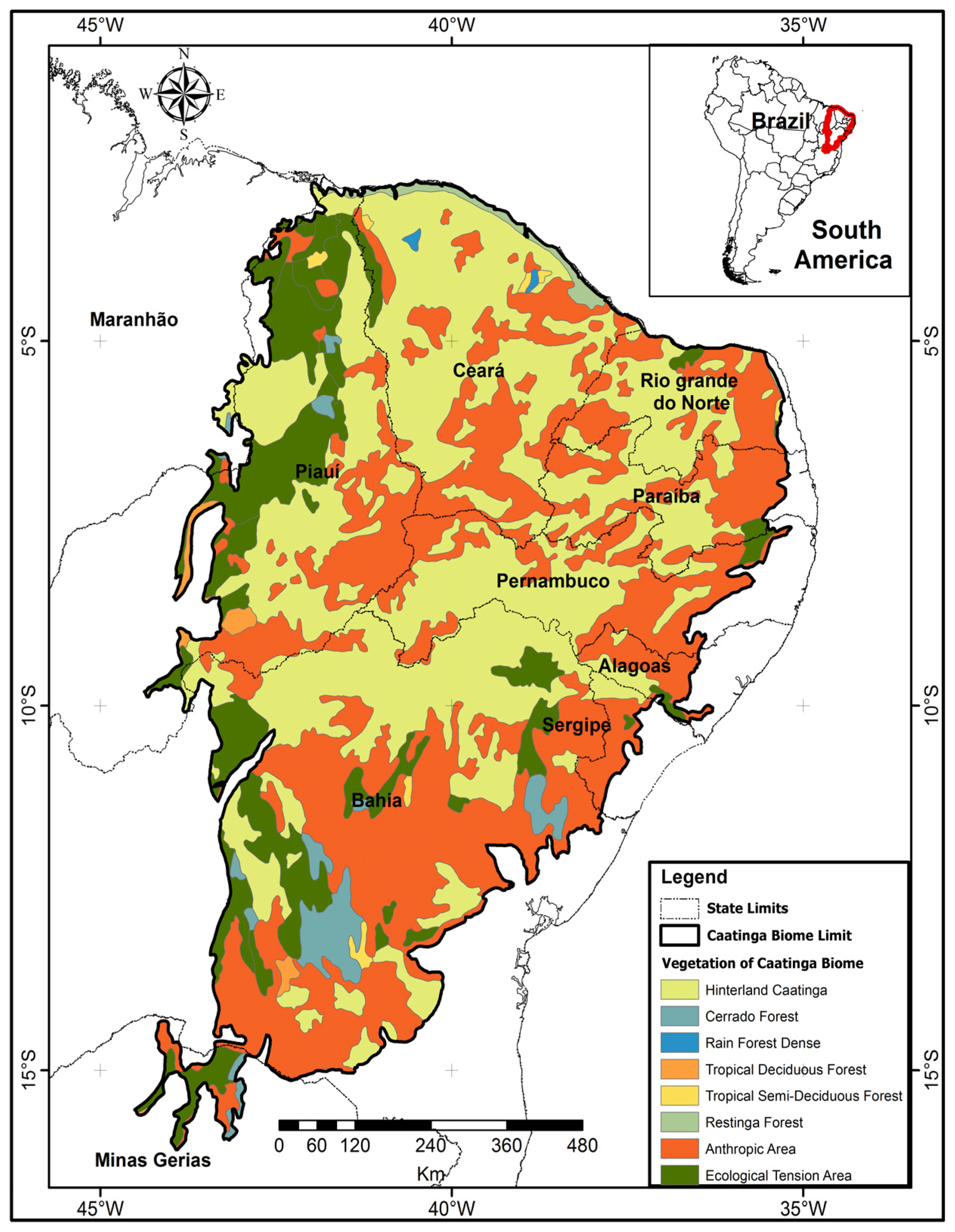
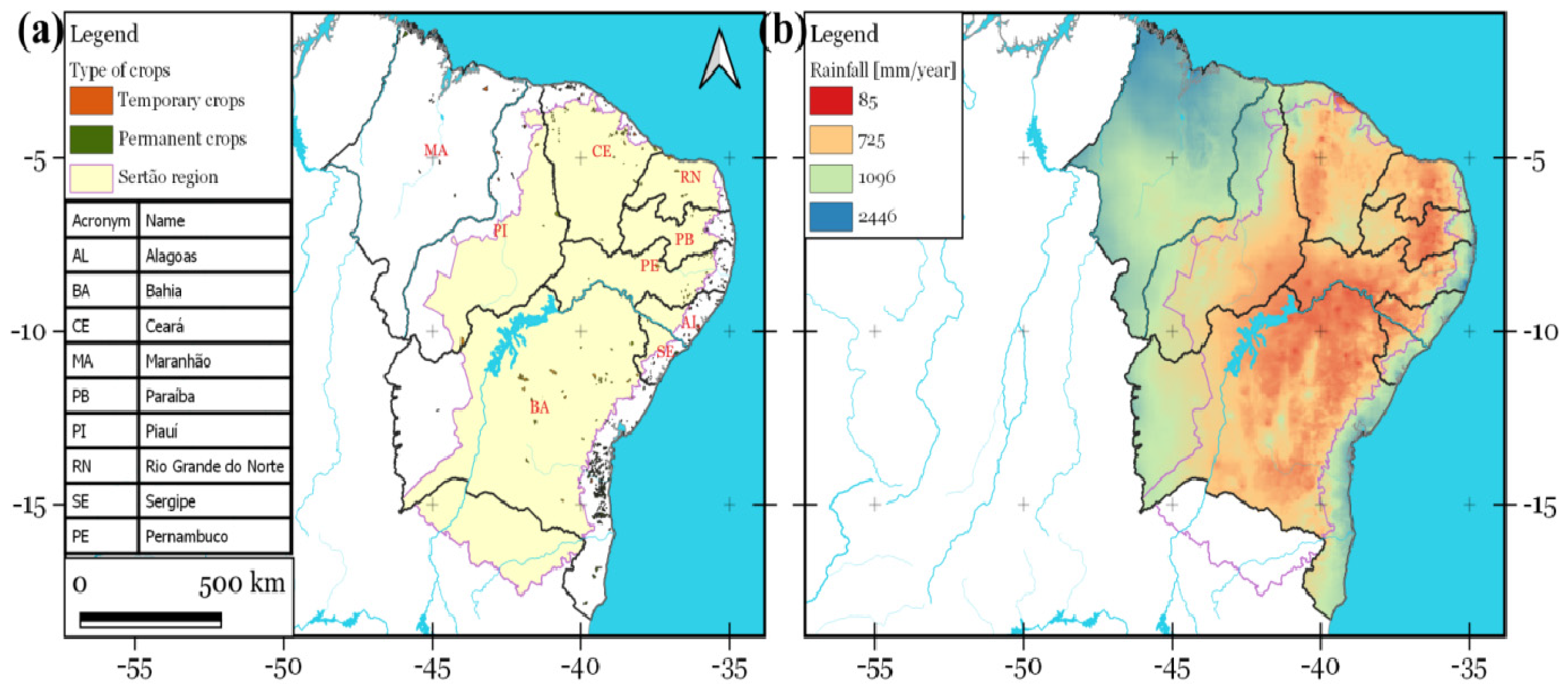
2.1. Study Area

The northeastern South America region is taken to encompass mainland South America between the parallels 1° and 18° S and the meridians 35° and 47° W and spans a total area of 1.6 million km2 (see Figure 1). It is home to around 53.1 million individuals [47]. It represents a large geographical area covering a semi-arid climate with low and irregular rainfall, high temperatures, and high evaporation rates [48]. Within the region, other types of climates exist, depending on location, relief, and vegetation influences [11].
The climate pattern of the northeastern South America region is characterized by a transition in rainfall from the dry inland (Caatinga biome; Figure 1) to the humid Atlantic coast (Mata Atlântica biome). Mean annual rainfall increases steadily from less than 800 mm in the semi-arid interior to 1800 mm at the coast (Figure 2b). The semi-arid area covers 60% of the region. Within the northeastern South America region, the wettest season typically occurs from December to April, while the dry season extends from July to October [49]. The rainfall regime is mainly influenced by the seasonal migration of the Intertropical Convergence Zone (ITCZ), the El Niño Southern Oscillation (ENSO), and the Tropical North Atlantic sea surface temperature. Severe droughts happened during El Niño events in 1983, 1998, and 2016, and due to warm surface waters in the Tropical North Atlantic between 2012 and 2018 [50].
Vegetation within the northeastern South America region was classified into several land cover types, including both unmanaged native and managed agricultural vegetation (Figure 1 and Figure 2a). The four most prevalent land cover types within the northeastern South America are Caatinga, Cerrado, Atlantic Forest, and Amazon Forest, covering 52.5%, 29.4%, 10.7%, and 7.4% of land area, respectively [30]. The Caatinga ecosystem (Figure 1) covers 735,000 km2 of northeastern South America region and is characterized by a mosaic of xerophytic vegetation [49]. The term “Caatinga” (Caa = forest, tinga = white) comes from the Tupi language and is used synonymously with Steppe Savannah as defined by Trochain [50]. Typical Caatinga is composed of woody vegetation with a discontinuous canopy (three to nine meters). Most Caatinga plants are formed with a fearsome array of thorns that emerge from microphyllous foliage lost during periodic droughts. The ground layer is rich in bromeliads, annual herbs, and geophytes. Typical species include Amburana cearensis, Anadenanthera colubrina, Aspidosperma pyrifolium, Poincianella pyramidalis, and Cnidoscolus quercifolius [11].
One prominent feature observed in the Caatinga land cover during a prolonged period of drier-than-normal rainfall conditions is a gradual weakening in vegetative greenness [51]. The vulnerability of the Caatinga to periodic droughts is further exacerbated by high levels of habitat degradation [29]. Indeed, the biome is one of the most threatened in the northeastern South America region due to widespread deforestation for farming and mineral extraction [52]. Despite the fauna and flora of the Caatinga biome region being clearly adapted to periodic droughts, some scientists believe that they may already be operating at their physiological limits [50]. Prolonged and frequent occurrences of droughts present significant challenges to flora and fauna [53].

2.2. Datasets

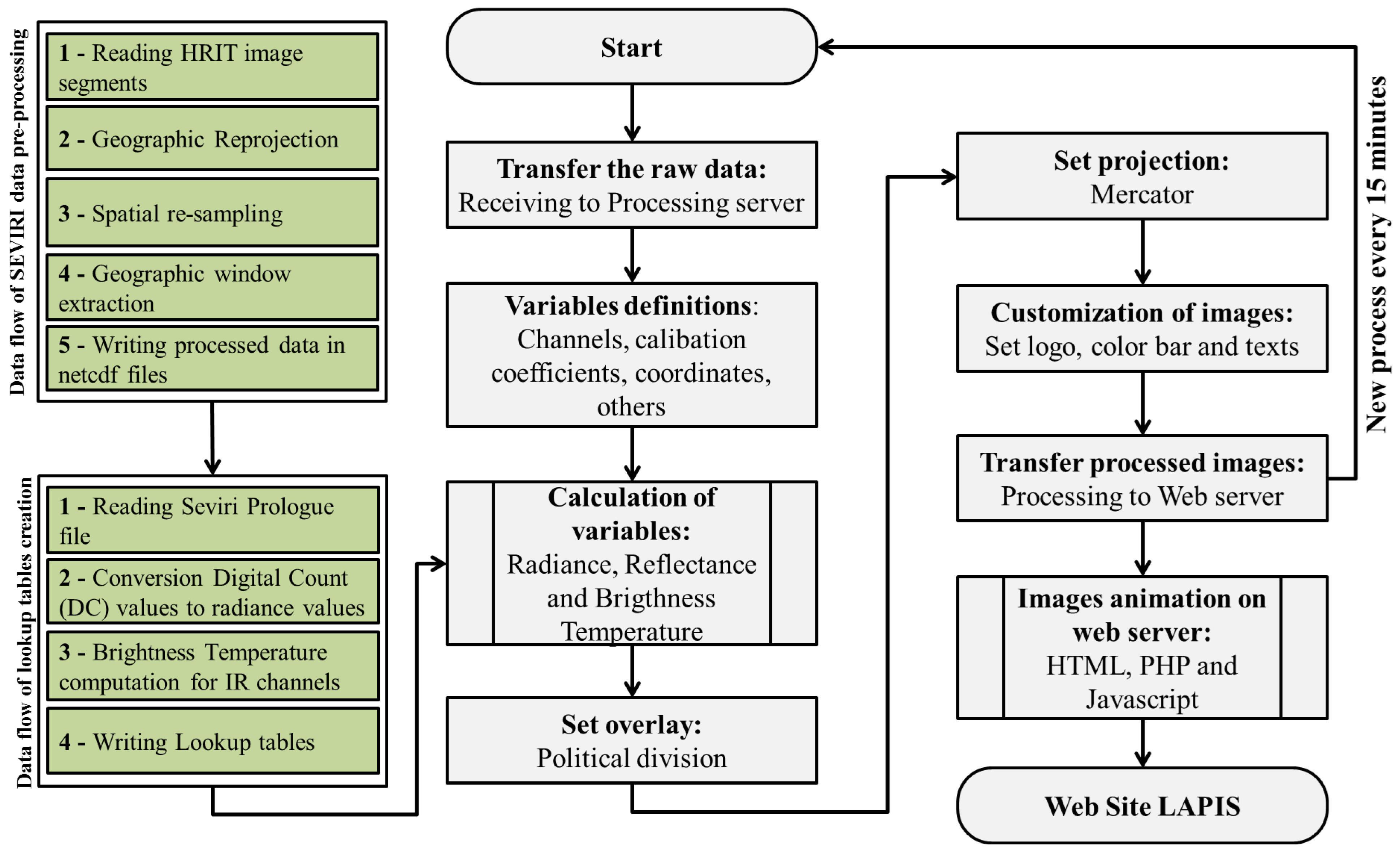
2.2.1. Meteosat SEVIRI NDVI Data from EUMETCast Service

Meteosat second generation (MSG) spinning enhanced visible and infrared imager (SEVIRI) NDVI-derived pentad NDVI data used in this study are composed of daily NDVI data [51,54]. These data are produced by the European Organization for the Exploitation of Meteorological Satellites in Darmstadt, Germany, which uses the processing method originally proposed by Ertürk et al. [55]. They are then uplinked to the SES-6 communication satellite in wavelet compressed format. The Laboratório de Análise e Processamento de Imagens de Satélites (LAPIS) of the Universidade Federal de Alagoas (UFAL) receives and archives these data in compressed form on drivers accessible through personal computers on the network (Figure 3).
MSG satellites have measured operationally shortwave and longwave radiation from the Earth and its atmosphere on eleven instrument channels with a time frequency of 15 min since 2003 [56]. Data from the operational missions of the MSG 1-4 satellites, located near 0° longitude (Gulf of Guinea), were used for the purpose of this study. A pentad data frequency (i.e., the mean over 5 days) was chosen for the correct sign of the vegetation-precipitation relationship at a regional scale to provide sufficient statistical significance with a moderate computational effort [31]. Over the entire study area and 18-year period, we composited daily SEVIRI NDVI to the monthly one for comparison with the drought index by computing the average value of daily NDVI within a single month.
18 years of monthly-pentad MSG SEVIRI NDVI were obtained through the LAPIS/UFAL (https://lapismet.com.br/dados/ accessed on 25 September 2023). The operational NDVI product derived from the SEVIRI Level 1.5 image data for VIS0.6, VIS0.8, and IR10.8 data is part of an automatic processing approach developed by [31,55]. The original data were corrected: (1) for all data, (2) atmospheric correction performed, (3) Bidirectional Reflectance Distribution Function (BRDF), (4) adjacency correction performed, and (5) low or average aerosol quantities. The MSG SEVIRI NDVI was defined by Barbosa et al. [31].
For the MSG images, NDVI was extracted from the single grid cell that encompasses the northeastern South America boundaries as a mask; a total of 18,399 grid cells were extracted and resampled as a numerical matrix (number of grid cells versus one column for each monthly composite). The NDVI time series was denoted as NDVIijk, where i is the month (i = 1…12) or i is the five days (pentad) (i = 1…73), j is the year (j = 2004…2022), and k is the grid cells (k = 1…18,399), and was transformed to a matrix of monthly NDVI anomalies (NDVIaijk) with respect to the 2004–2022 base period. NDVIa time series [17] were then scaled by the standard deviation, as follows:
N D V I a i j k = N D V I i j k N D V I i k ¯ 1 ( n 1 ) ( N D V I i j k N D V I i k ¯ ) 2
The matrix of standardized NDVI anomalies (i.e., SDVI [17,57]) was referred to as the NDVIa matrix (number of grid cells versus number of months, pentads, or days). Because spatially complete information at high temporal resolution is of crucial importance to support the statistical analysis, the choice of SEVIRI-calculated grid size resolution is a compromise between achieving the highest possible resolution at the daily timescale and still maintaining regional to local scales to guarantee pixel information in almost all grid cells. Most importantly, however, a previous study by Barbosa et al. [31] showed that the SEVIRI NDVI derived from the daily 1.5-data serves as a good proxy for rainfall activity in the northeastern South America region during the rainy season months.
In the next step, linear least squares trend analysis of visible (0.64 µm) and infrared thermal (10.8 µm) radiances from the pentad-SEVIRI spectral images was performed on the 5-daily composite for each pixel (see Figure A1 in Appendix A). The calibrated and geolocated (level 1.5) radiance is a compressed version of the original data with a resolution of 3 km under the nominal field of view of Meteosat at 0 degrees longitude, every 15 min for the 2004–2022 period. A few pentads are missing in the level 1.5 dataset, which, together with the high-resolution resampling, occasionally resulted in pixel cells without information. Daily 1.5-data for a full scan were only used at 1200 UTC (late morning) because it leads to near-polar orbiting time that crosses over the equator at approximately 1200 UTC. Only trends with Pearson correlation coefficients significantly different from zero (at significance level p < 0.05) are considered significant trends.

2.2.2. SMOS Surface Soil Moisture Data

Soil moisture and ocean salinity (SMOS) mission is an L-band passive microwave satellite dedicated to global surface soil moisture (SSM) measurements [58]. It contains global daily soil moisture data with a spatial resolution of ~25 km, in 0–5 cm of the soil layer, in m3/m3, from June 2000 to the present. SSM is a vital index for many applications concerned with monitoring drought events [22]. For this study, the daily SSM estimates were extracted from the SMOS-level-3 product provided by the Barcelona Expert Center (https://bec.icm.csic.es/ accessed on 25 September 2023). These data were averaged considering their ascending and descending orbits to minimize the effect of radio frequency interference (RFI) on the retrieved SSM values [59]. The level-3 SSM product is a set of several algorithms. A short summary of the main features of this product is provided in [59]. The choice of this product was based on its acceptable performance in the identification of drought when compared to in situ measurements in the study area [60].

2.2.3. Climate Data

For the study area, rainfall and temperature data were extracted from the single grid cell that encompasses its geographical coverage in the ERA5–Land and IMERG late run (integrated multi-Satellite retrievals) datasets, respectively. Both datasets were produced by the ECMWF (European Center for Medium-Range Weather Forecasts) and the Global Precipitation Mission (GPM) with a spatial resolution of 0.1°, respectively. The IMERG v6 product provides daily estimations of rainfall from multiple satellite-based observations and is commonly used in hydrological studies [61]. This version of IMERG was selected because it has shown a good rainfall representation over the study region, improving on other satellite and reanalysis products (e.g., [62]). Hence, the final IMERG v6 product is a gauge-corrected product, but here it was not further corrected with its station data. Since the meteorological observation network in the study area is sparse and depends on the availability of archives [50].
The IMERG (version 6 on a half-hour 0.1°) gridded product was accessed on NASA’s Goddard Space Flight Center (https://pmm.nasa.gov/data-access/downloads/gpm accessed on 25 September 2023) [63]. In this study, the IMERG gridded data were averaged to daily timescales and then to a monthly resolution. This gridded data was averaged following the same interpolation procedure as the one used in the SEVIRI-derived NDVI data. Additionally, daily rainfall data from 30 weather stations across the study area were used as reference data for qualitative assessment. The stations were selected from a set of rainfall data belonging to the Brazilian Meteorological Institute and available from the official webpage (https://portal.inmet.gov.br accessed on 25 September 2023). Specifically for the ERA-gridded product, temperature data were averaged to a monthly resolution and then used to calculate climatology and anomalies. All the datasets above have a time range of 2004–2022.

2.3. The Standardized Precipitation Index (SPI)

The SPI, proposed by McKee et al. [64], is an index that monitors drought conditions by exclusively considering rainfall data. It is commonly used to monitor meteorological droughts. In this study, the SPI was calculated based on the quarterly scale (SPI-3), because the NDVI lags rainfall [65]. This lag correction between both variables is related to the water storage capacity of the soils [49], but this aspect is beyond the scope of this study. The rainfall time series is initially fit to a gamma distribution, which is then transformed into a normal distribution using an equal probability transformation [36]. Daily rainfall estimates (mm) from the IMERG v6 product over the study area were used over the period 2004–2022 for the construction of the SPI [64]. In general, negative SPI values indicate a dry period, and positive values indicate a wet period. The SPI-3 time series were structured in one numerical matrix referred to as the SPI3 matrix, based on Barbosa et al. [51]. The probability density function for the gamma distribution is given by the expression:
g ( x ) = x α 1 e x / β β α Γ ( α ) ,       f o r     x > 0
where α > 0 is the shape parameter, β > 0 is the scale parameter, and x > 0 is the total accumulated precipitation over a three-month period (called the time scale). Γ(α) represents the gamma function, which is defined by the integral [66]:
Γ ( α ) = 0 y α 1 e y d y
The gamma function was evaluated either numerically or using tabulated values depending on the value of α. A maximum-likelihood estimation based on the method of L moments was used to estimate parameters α and β [67]. The probability density function, g(x), is then integrated with respect to x to obtain an expression for the cumulative density function, G(x), which represents the accumulated rain that has been observed for a given month and time scale:
G ( x ) = 0 x g ( x )     d x = 0 x x α 1 e x / β β α Γ ( α ) d x
Although negligible rainfall amounts are frequent in northeastern South America [68], G(x) is not defined at x = 0 [69]; therefore, G(x) was calculated following the approach of Stagge et al. [70]:
p o = n p n + 1
D ( x ) = p 0 + ( 1 p 0 )   G ( x ) ,       f o r   x > 0
D ( x ) = n p + 1 2 ( n + 1 ) ,       f o r   x = 0
where np refers to the number of zero-rainfall events, n is the sample size, po is the observed likelihood of zero-rainfall events, and D(x) is the cumulative density function for observed precipitation. Finally, D(x) is transformed into a normal standardized distribution using a zero mean and unit variance, from which the SPI drought index using the 3-pentad time scale (SPI3) was obtained.

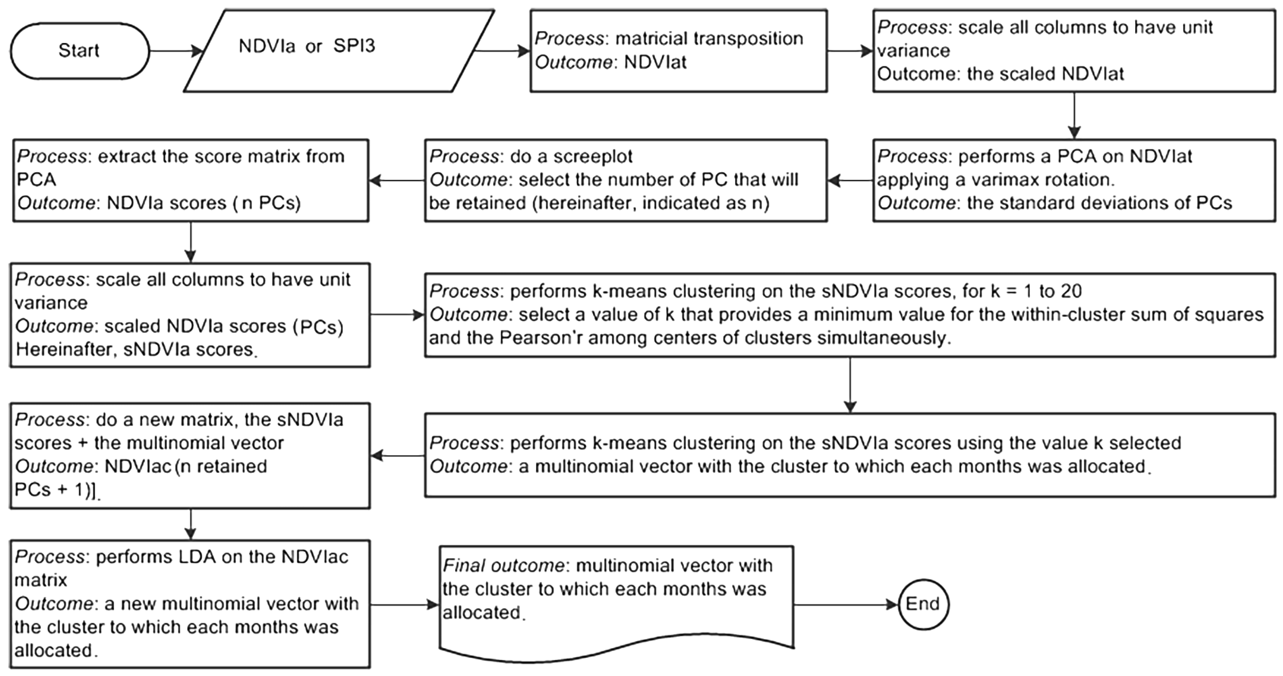
2.4. Statiscal Analyses

To understand the regional scale on vegetation response to rainfall extremes on the magnitude of anomalies in NDVI and SPI3, the statistical analyses over northeastern South America were computed using the 18-year NDVI rainfall anomalies from 2004 to 2022. The approach was carried out in four main steps as a response to seasonal and interannual variations in hydroclimatic conditions across space. The first step involved rearranging the NDVIat and SPI3t matrices to obtain two matrices that are referred to as NDVIat and SPI3t, respectively. During the second step, a principal component analysis (PCA) was applied to the NDVIat and SPI3t matrices. PCA was performed by computing the eigenvectors of the covariance matrix, while the varimax method was used to provide an orthogonal rotation.
It is important to note that the original PCs were associated with an arbitrary coordinate system. The rotation procedure changes the PCs to another coordinate system that yields a better separation of the PCs in the spatial context [51]. Unlike other orthogonal rotations, the rotation maximizes the sum of the variances of the squared loadings (squared correlations between variables and PCs) [71]. The number of PCs retained was based on screen plots for NDVIa and SPI3, which show the variances for each against the number of PCs (criterion known as the Kaiser’s rule).
The principal component scores for the retained PCs were computed and resulted in two matrices, which are referred to here as NDVIat and SPI3t scores, respectively. Each score matrix has a dimension equal to rows × n PCs, where n is the number of retained PCs. The score matrices were scaled by column during the third step of this approach by the mean and the standard deviation.
A canonical analysis (CA) was then performed on the NDVIat and SPI3t score matrices. The k groups used are based on two criteria: (a) minimization of the sum of squares of distances between each grid cell and the assigned cluster center, and (b) verifying that the linear correlation coefficient between the centers of clusters is less than 0.36 [72]; if the algorithm did not converge based on this criterion, then the first relative minimum that was found was selected [73]. The algorithm of Hartigan and Wong [74] was used to perform the iterations, and the Euclidean distance was used as the distance measure.
The fourth and final step involved combining the NDVIat scores matrix (216 × n retained PCs) with the NDVIa clusters defined by the CA (represented by a row × 1 multinomial vector), which resulted in a matrix that is referred to as NDVIac [column × (n retained PCs + 1)]. A discriminant model that considers the multinomial vector as a factor specifying the class for each observation and the scores of retained PCs as discriminators was then fit [75]. The moment method has been used to standardize estimators of the mean and variance. The clusters with different classifications were re-coded according to discrimination based on linear discriminant analysis (LDA). The LDA was then applied to the SPI3 score matrix as well. The final products of this approach were two multinomial vectors containing the classifications for NDVIa and SPI3 variables at monthly scales.
Overall, eight PCs retained 46 percent of the variance for NDVIa, while eight PCs retained 80 percent of the variance for SPI3. The clustering based on the k-means method identified eight similar groups for the NDVIa and SPI3 variables. The LDA-based classifier improved the CA-based discrimination; e.g., the NDVIa variable has been structured in the groups N1, N2, N3, N4, N5, N6, N7, and N8, which contain 20, 55, 36, 40, 30, 15, 82, and 104 members, respectively, while the SPI3 variable has been reduced to the groups S1, S2, S3, S4, S5, S6, S7, and S8, which contain 44, 62, 56, 32, 49, 57, 49, and 33 members, respectively. Figure 4 shows a flowchart that illustrates the procedure described above.
It should be noted that the order of the identified clusters (N1 to N8) is not related to the spatial average of the NDVIa or SPI3 in the northeastern South America region; the order has been defined randomly by the applied algorithms used during the discrimination process while only considering the similarity between members as a criterion for clustering. Therefore, these clusters have been reclassified based on the median calculated from spatially averaged SPI3 and NDVIa values over NE South America (Figure 5 and Figure 6) and will be referred to as patterns throughout the remainder of this study. The median was chosen for this purpose as it allows splitting the upper half of the NDVIa or SPI3 time series averaged over the entire northeastern South America region from the lower half.
This approach has linked the clusters N1, N2, N3, N4, N5, N6, N7, and N8 with the NDVIa patterns F5, F4, F7, F1, F6, F8, F2, and F3; and the clusters S1, S2, S3, S4, S5, S6, S7, and S8 with the SPI3 patterns F2, F6, F1, F8, F4, F7, F3, and F5. It is important to note that this new order provides information concerning the dominant process that is taking place, e.g., regarding the NDVIa patterns, F1 indicates the occurrence of a widespread greening over all northeastern South America region (highest median), while F8 indicates the occurrence of a widespread browning in the entire study area (lowest median). Similarly, for the SPI3 patterns, F1 indicates the occurrence of widespread wet conditions over the northeastern South America region (highest median), while F8 indicates the occurrence of widespread drought conditions over the northeastern South America (lowest median).

3. Results and Discussions

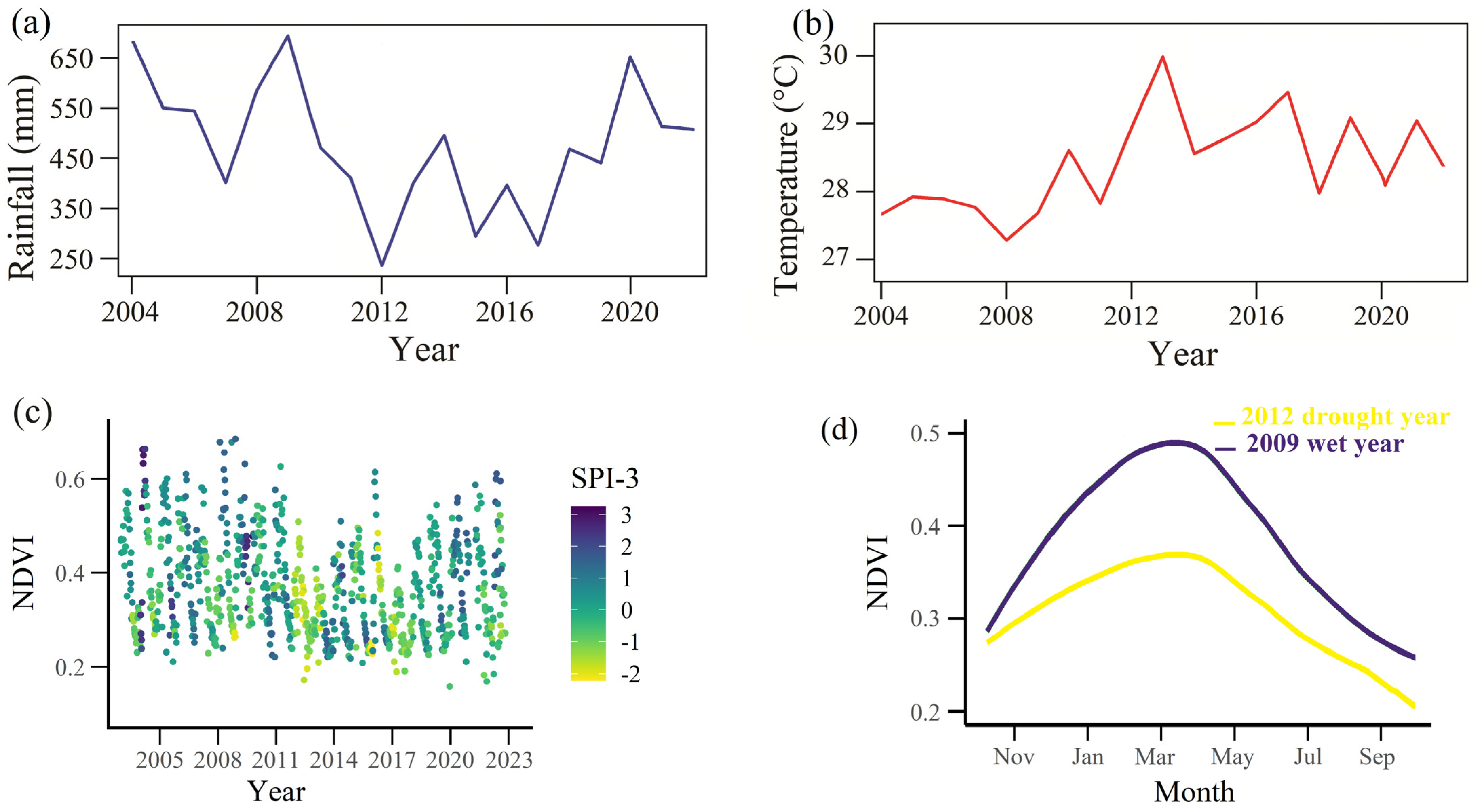
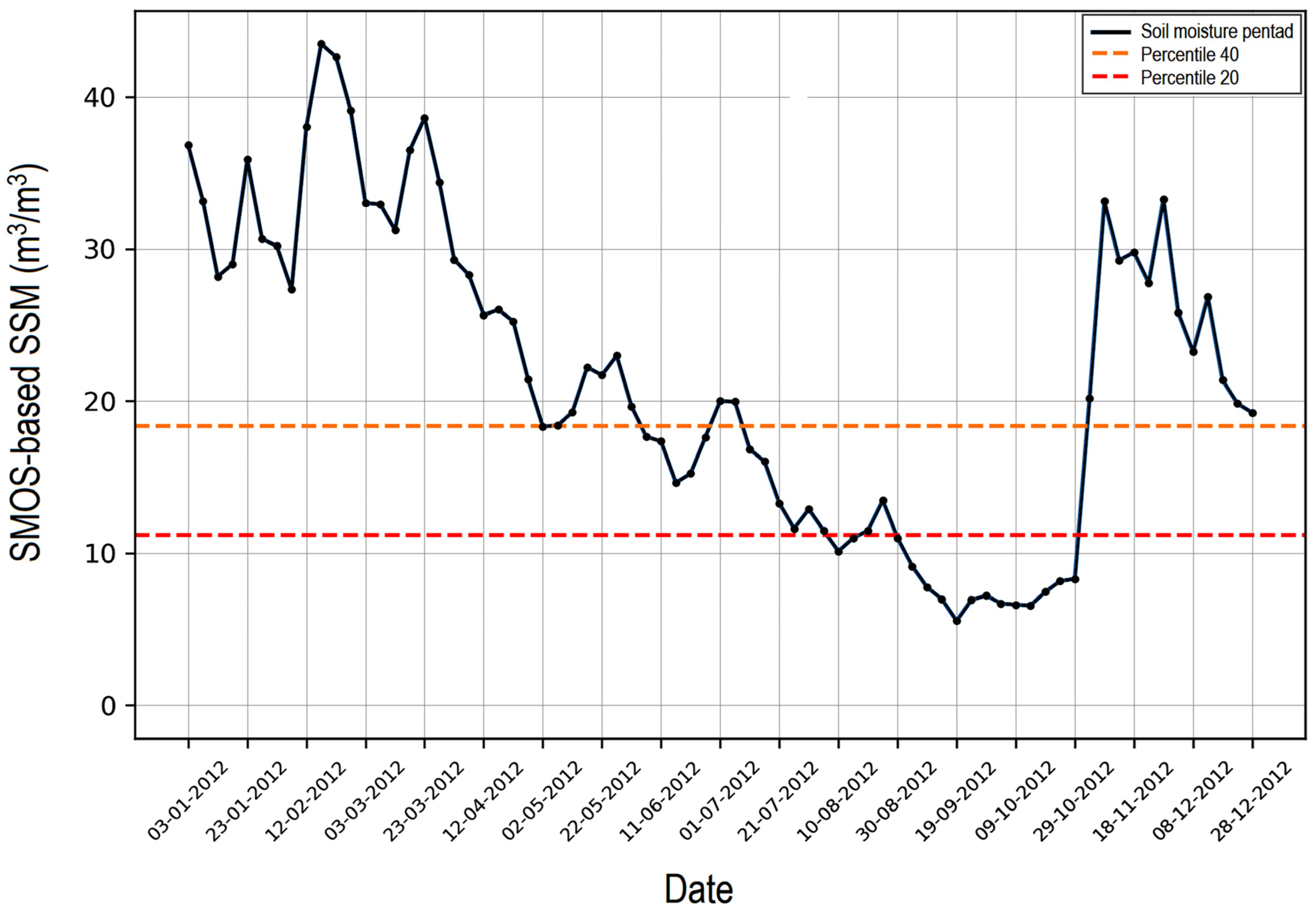
3.1. The Impacts of Flash Drought Events on Vegetation Dynamics

A visual inspection of Figure 7c,d shows the seasonal and interannual variations in NDVI and SPI-3 indices over the entire northeastern South America region from 2004 to 2022. Regional analysis revealed that drought and wet cycles had considerable impacts on vegetation dynamics (i.e., here defined as fluctuations in phenology and biomass). The SPI-3 drought index shows that the study region experienced intensified drought in the second decade of the 2000s, with 2012 and 2017 among two of the three worst droughts since 2004 (Figure 7). Annual rainfall was below the 18-year term average during the entire 2012–2017 period. This dry period was broken dramatically by a moderate La Niña event in 2020, with regional average annual rainfall surpassing the 18-year term average by nearly 190 mm. These findings were also supported by a linear least squares trend analysis of visible (0.64 µm) and infrared thermal (10.8 µm) radiance images from the time series of pentad-SEVIRI spectral channels revealed a negative trend in measured radiances for the visible radiances over large areas of the northeastern South America region, which was suggested as a reduction in clouds in the 18 years of the study. Increased radiative losses are clearly implicated in this enhanced drying, which enhanced atmospheric evaporative demand, coupled with below-average rainfall in 2012 and 2017 (see Figure A1 in Appendix A). This could explain vegetation stress or vegetative drought [33,34], mostly in the Caatinga biome, induced by increased temperature and radiation and amplified by a reduction in rainfall [50].
Overall, the second decade of the 2000s warm and dry periods spanning the northeastern South America region were characterized by below-average rainfall and anomalously higher temperatures, representing a drought response to warming. Significant negative trend (p < 0.05) in annual rainfall of −1307 mm·year−1 and significant positive trend (>95th percentile) in annual air temperature of 0.762 °C·year−1 were identified for the period 2004–2022 (Figure 7a,b).
There is ample evidence of differential responses of vegetation phenology to drought (i.e., SPI-3 < −1) and wet extremes (i.e., SPI-3 > +1) over the northeastern South America region; growth enhancement in vegetation is strongly controlled by water availability (Figure 7c). An overall reduced seasonality of vegetation phenology was detected from 2012 to 2017 (Figure 7c). In contrast, a general increase in vegetation seasonality, dominated by the wetter-than-average periods of 2004–2011 and 2018–2022, was identified. Additional changes in rainfall not only affect vegetation activity but also decrease vegetation phenology, as indicated in the shape and magnitude of seasonal NDVI profiles on the regional scale (Figure 7d).
Yet there is evidence that there is some correspondence between the interannual variability of rainfall and noticeable seasonal differences in the NDVI extreme profiles. Over the entire study area and 18-year period, there was a decreasing trend in NDVI of over 17%. The results showed abrupt shifts in vegetation activity between dry and wet rainfall variations. Periods of drought breaks and the persistence of low vegetation growth were prominent, particularly after the onset, thus exposing the region to the impacts of flash droughts. The rapid and sudden responses of ecosystems to droughts have been found in Australia (e.g., [76]) and other global regions (e.g., [5]). These findings together highlight the need for models to explicitly consider drought-induced abrupt shifts in vegetation activity and vegetation dynamics for predicting future ecosystem states, particularly in tropical semiarid regions where rainfall is highly variable and vegetation dynamics is limited by soil moisture.
The drought that affected this study area in 2012 was the most extreme in the period from 2004 to 2022, as indicated by consecutive negative SPI-3 lasting for 9–10 months (Figure 7c). Another way to look at the 2012 drought year is by computing soil moisture derived from remote sensing observations to describe the onset and termination times of this drought. The duration and interval of the data set processed is presented in Figure 8. Rapid and dramatic declines in soil moisture resulted from a period of abnormally warm-dry weather conditions over the northeastern South America region with a peak SPI-3 intensity of −2.50 (Figure 7b). A notable bimodal distribution was observed, with the dry-wet abrupt transition (i.e., nearly-flat line below the 20th percentile that is equivalent to NDVI ≈ 0.3). This is shown in Figure 8 for the timing when soil moisture reaches the value equal to the 20th percentile after drying of soil moisture (i.e., onset time of a drought event) and the increases in the soil moisture prior to the 20th percentile plus the 20th percentile amplitude during the wetting-up phase (i.e., the end time of a drought event). Here, the length of the soil moisture deficit is calculated as the difference between the end time and onset times of a drought event.
A more quantitative method to identify the timing, duration, and intensification of the 2012 drought year can be computed through the rate of intensification using weekly soil moisture percentiles on the regional analysis [7,77]. This method may not analyze changes in drought per se, but changes in mean soil moisture can be inferred to be related to the occurrence of events with high soil moisture deficits. Under conditions of critical soil moisture deficits, the threshold adopted here is twofold: (1) soil moisture is less than the 40th percentile, and (2) the peak drought intensity must fall below the 20th percentile. Two relevant flash droughts were identified, which occurred from 4 June to 28 June (duration = 24 days) and 11 July to 31 October (duration = 114 days). The two flash drought events were a subset of the 2012 drought year (the SPI = 303 days from January to October). The rate intensification for the short-duration event (24 days) was relatively lower as compared to the high magnitude resulting from the long-duration event (114 days). In this analysis, flash droughts represented 46% of all droughts (SPI-3). A flash drought event was recognized when the absolute value of rate intensification of soil moisture retreated to the 20th percentile per week. Of the flash drought events over the 2004–2022 period, 88.9% experienced rapid intensification within 4 weeks of drought onset (Figure 8).
Here, SPI-3 variability is mostly driven by rainfall variability. SPI-3 is not intended to be a proxy of soil moisture but rather a flexible metric of vegetation water stress. Regardless of the time scale of the SPI-3, a drought event begins when SPI-3 ≤ −1.00 and persists until SPI-3 > −1.00; the value of −1.00 is the threshold value that differentiates dry vs. non-dry. In general, the lower the time scale, the higher its capacity to identify short-term droughts [48]. When the soil moisture content drops from the 40th percentile to below the 20th percentile are not less than 4 pentads (20 days), the NDVI exhibits values lower than 0.20. For example, if temperatures are abnormally high, evaporation increases, drying out soils beyond what would have occurred just from the lack of precipitation. This is particularly true for flash drought. Vegetation may play a critical role in flash drought self-intensification under dry conditions because it modulates soil moisture drying.
Spatial patterns in soil moisture and vegetation conditions are shown in Figure 9 and Figure 10 by the average pentad data of soil moisture content and values of NDVI over the two sub-seasonal changing periods in the 2012 flash-drought events. The results of the spatial analysis revealed a differential impact of flash drought events on vegetation dynamics, primarily over the Caatinga vegetation (highlighted by red areas in Figure 10). The drought resulted in reduced vegetation dynamics across 88% of the study area, of which 96% showed surface soil moisture content below 10 (m3/m3). The persistence of low soil moisture content is still prominent, thus exposing the northeastern South America region to the strong effects of flash droughts on vegetation dynamics, particularly over the Caatinga biome.
As shown in the Figure 9 and Figure 10 the values of NDVI are not changing uniformly over the study area, decreasing dramatically from the northwestern dry interior (where the vegetation was classified as xerophytic or Caatinga) to the open savanna (the Cerrado vegetation). Overall, the contrast of NDVI values between the eastern-coastal-forested areas and the Caatinga has strong spatial variability. Different locations with the same value of NDVI do not necessarily have the same vegetation greenness. However, regional changes in NDVI are not only governed by changes in soil moisture but also influenced by changes in land use (human signal). Yet, NDVI may be increased by irrigation, which can enhance vegetation activity in the short-medium term but may reduce resilience by increasing the risk of soil salinization. In much of the study region, flash drought events were identified if the values of NDVI were less than 0.3 and soil moisture became less than 10 (m3/m3) (i.e., the rate of soil drying). Robust declines in soil moisture occurred over Caatinga areas where the radiance in the solar measured by Meteosat decreased by about 0.608 W m−2 relative to the 2004–2022 period.
An additional and unique finding of this study is that soil moisture may play a role in drought self-intensification under dry conditions in which vegetation growth is dormant and leads to higher atmospheric evaporative demand, yet still maintains capability to contribute to the length of flash droughts [7,30,77]. In addition, a higher soil organic content normally promotes larger water holding capacity and a capacity to buffer against water deficits during flash droughts [78]. It further suggests that these mechanisms are not mutually exclusive and that their relative contributions to land-atmosphere coupling need to be assessed in future studies.

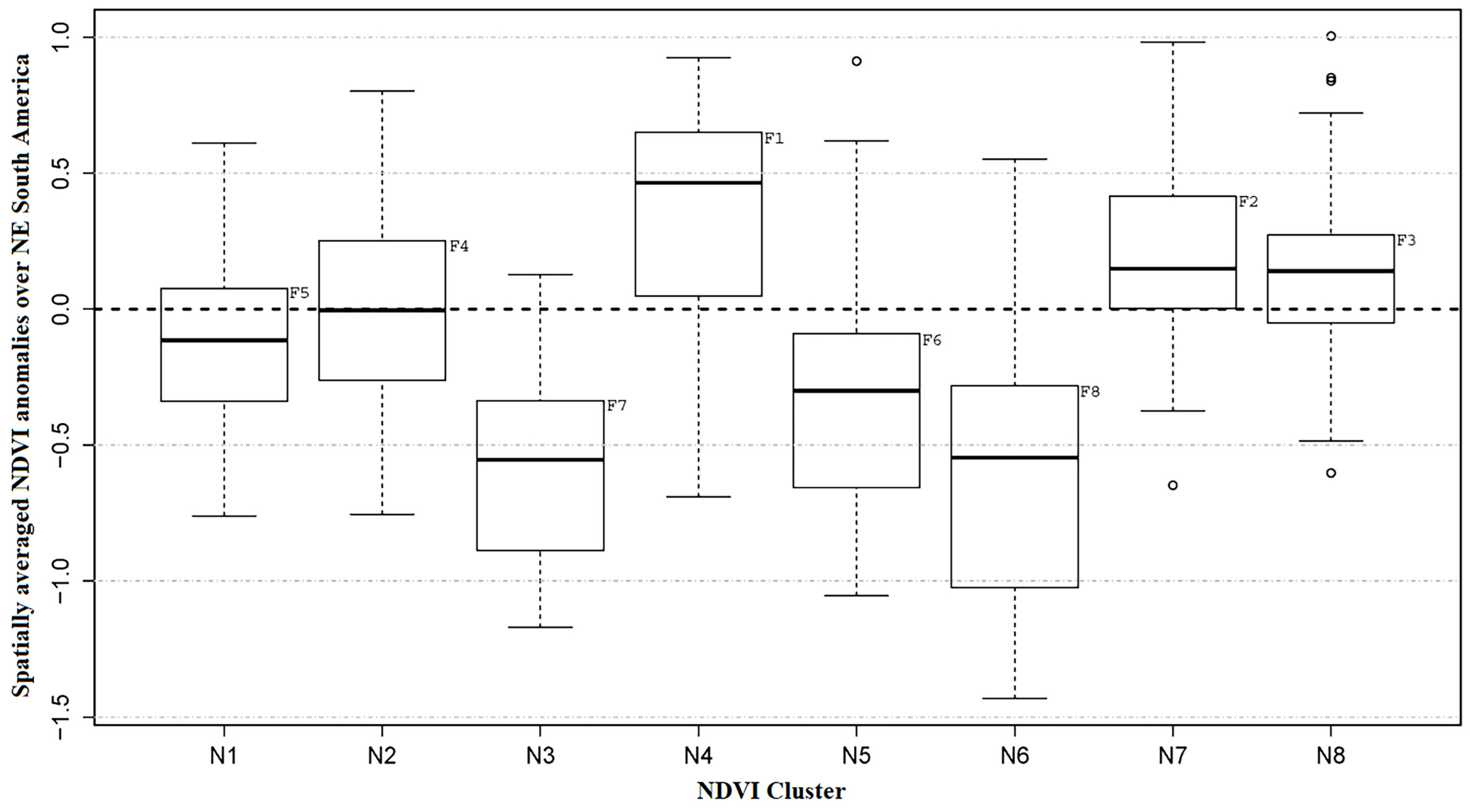
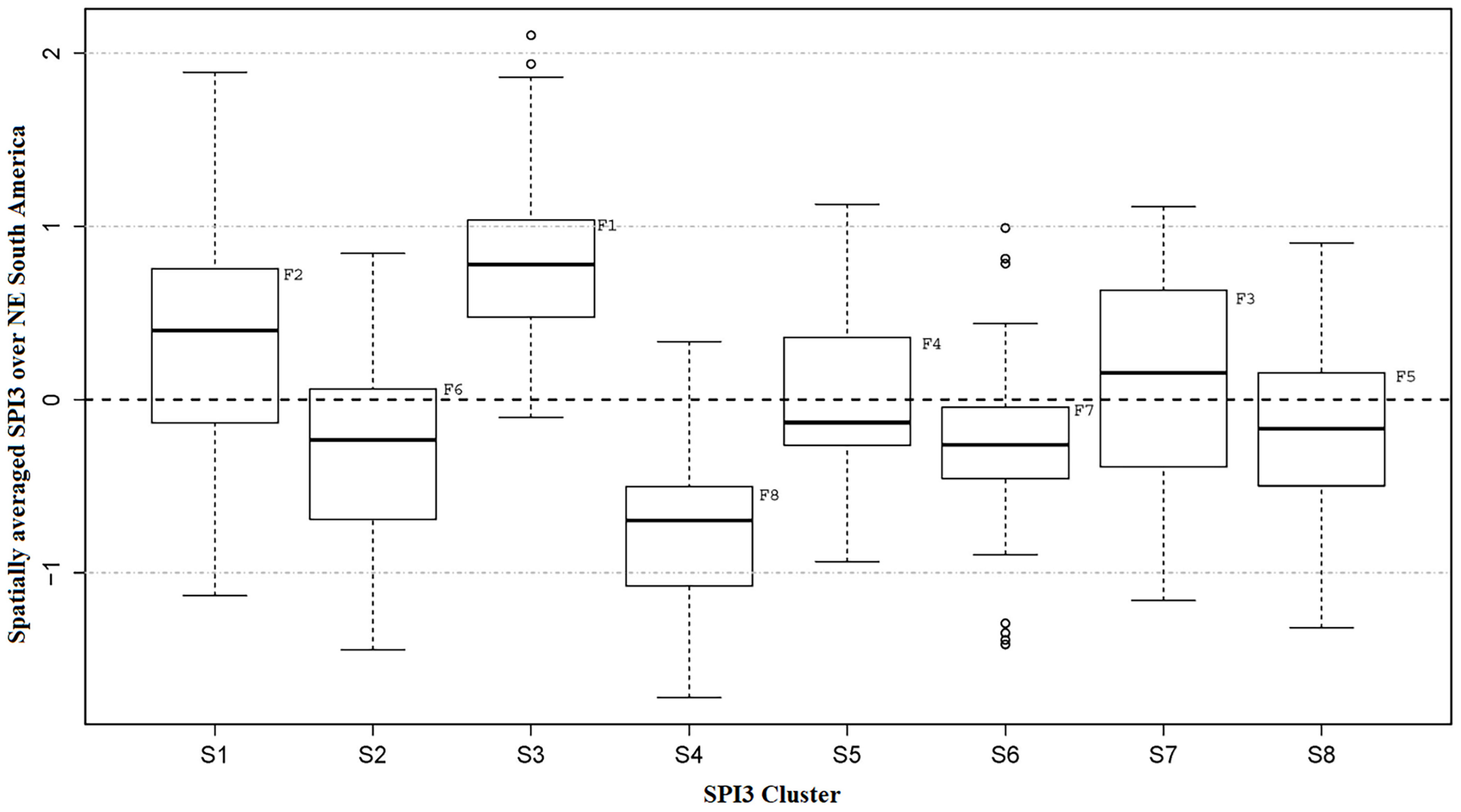
3.2. Ecogeographic Patterns in Vegetation Dynamics

Regional maps were generated to assess large-scale ecogeographical patterns in vegetation growth (monthly averaged NDVI anomalies; see Section 2.4) over the northeastern South American region (Figure 11). Changes in large-scale clusters of vegetation activity are difficult to isolate from local scales based on the pixel, thus justifying the use of statistical methods to capture the spatial and temporal features of gridded-NDVI anomalies. As a result, within the 2004–2022 period, eight sub-regions (N) were identified based on the cluster analysis. The regional centroids ranged from −0.55 to 0.47, whose seasonal domains (F) are defined in Figure 5. The corresponding maximum, median, and minimum area averaged-NDVI anomalies are shown in Figure 5. The regional response of the NDVI anomalies varies widely and is also dependent on its ecogeographical environment. The ecogeographical distribution of these sub-regions can be classified as N4, N7, or N8 (with positive centroids) for greening vegetation, and the distribution can be classified as N1 to N3, and N5 or N6 (with negative centroids) for browning vegetation.
Among the eight sub-regions through multivariate analyses, the sub-region where the average anomaly of NDVI is greater (cluster centroid) is N4, and it is associated with the green-up pattern (F1). Nonetheless, it is clear from Figure 5 and Figure 11 that N6 is characterized by the lowest anomaly of NDVI; it has the brown-down pattern (F8). Visually comparing variations of the NDVI anomalies (Figure 11) shows that ecogeographical transition zones between green-up and brown-down environments are identified, which also exhibit differential responses of ecosystems to humid and drought conditions across space and among the main land cover types (Caatinga, Cerrado, Atlantic Forest, and Tropical Rainforest) of the study area. It is apparent that changes in the brown-down areas were dependent on land cover types, increasing dramatically from the northeastern dry interior (where the vegetation was classified as xeric scrubland and open thorn forest) to open shrub woodland. Additionally, these brown-down areas are dominated by Caatinga’s species, which are highly sensitive to drought variability, land use, soil properties, and topography. For example, vegetation on loamy soils responded much more to drought conditions than other soils [11,48,49].
Given that northeastern South America’s ecosystems are affected by rainfall variability on a sub-regional level, it is natural to consider to what extent this variability can be attributed to either climatic variability or human-induced environmental change. This variability was evaluated through a multivariate analysis of the spatial distribution for NDVI (Figure 11) and SPI-3 (Figure 12) anomalies. The size and magnitude of the different clustering groups did not differ much between the NDVI and SPI3 data analyses. The intra-regional variability (F1 and F8 ecogeographic patterns) between NDVI and SPI3 anomalies across extreme humid and drought conditions were very similar, as shown in Figure 7. However, the spatial distribution was not always the same. All the F2, F3, F4, F5, F6, and F7 patterns for the NDVI and SPI3 anomalies were found to considerably differ among them. This is largely attributed to the fact that an increase in rainfall does not result in higher green-up because northeastern South America’s ecosystems are also covered with evergreen species, or, the other way around, a decrease in rainfall does not result in further brown-down because these ecosystems are already covered with minimal vegetation growth. The influence of rainfall on the variations of NDVI was low, and perhaps human factors (land use change and landscape disturbance) have a stronger impact on all the patterns from F2 to F7.
Quantitative results from multivariate analysis showed that vegetation activity (the NDVI signal) across the Caatinga biome was highly sensitive to flash drought events. Additionally, despite their typically xerophytic characteristics, the plants of Caatinga react strongly and rapidly to low rainfall [49]. This is largely attributed to its highly drought-adapted hydraulic architecture and its ability to plug deep soil moisture reserves with its lengthy root systems [79]. For instance, grassland, xerophytic thorn savanna (shallowly rooted plants), and shrub woodland (deeply rooted plants) responded differently to drought conditions. Most of the studies based on the rainfall and NDVI relationship are valid for woody vegetation, but herbaceous vegetation composition also seems to be responsive to drought conditions in a similar way [80]. Here, it was also found that the negative NDVI anomaly pattern identified the influence of flash droughts on Caatinga vegetation stress because water scarcity can negatively affect vegetation activity, thus corresponding to NDVI below 0.30. Although based on different methods, this finding agreed well with a recent study [81] that found that Caatinga vegetation within the study region is highly sensitive to soil moisture.

4. Conclusions

To characterize the impact of flash droughts on vegetation coverage, this study assessed the influence of soil water deficits on vegetation dynamics in the northeastern South America region by combining time series of the vegetation index, rainfall, and soil moisture based on satellite remote sensing products at a daily time scale. An 18-year analysis, from 2004 to 2022, of the Normalized Difference Vegetation Index (NDVI), Standard Precipitation Index (SPI), and surface soil moisture (SSM) was performed based on three different satellite remote sensing estimates: the spinning enhanced visible and infrared imager (SEVIRI), the integrated multi-satellite retrievals algorithm (IMERG), and the soil moisture and ocean salinity (SMOS).
All analyses revealed that flash drought events exerted dramatic impacts on terrestrial ecosystems in the northern South America region during the first two decades of the 2000s, with changes in seasonal and regional vegetation dynamics. The fixed-threshold values to characterize flash drought events were suggested as the timing when the water deficit was less than −1.0 units and vegetation index reached a value equal to +0.3 during five consecutive weeks or more, coupled with soil moisture rates below 40% percentile, leading to a strong region-wide drought.
Furthermore, the linear least squares trend analysis of visible (0.64 µm) and infrared thermal (10.8 µm) radiances from the pentad-SEVIRI spectral images revealed a negative trend in measured radiances for the visible radiances along the entire central area of the study region, which was suggested as a reduction in clouds in the 18 years of the study. Radiance at 10.8 µm showed significant (p < 0.05) positive trends in large areas in the northern part and the coastal areas of the study region. The negative relationship (Pearson correlation of −0.62) between visible and infrared thermal in the study region’s semi-arid ecosystem (i.e., the Caatinga biome), where biomass production is determined by the amount of rainfall, and the opposite in its coast areas, where rainfall is not the limiting factor for vegetation growth, is consistent with findings of other authors, such as [82]. An alternative explanation was due to decreases in aerosol concentrations in the study region (e.g., [83]).
Nevertheless, the trend analysis must be considered very carefully since SEVIRI spectral radiances are affected by considerable uncertainties (e.g., instrumentation change, satellite drift, merging techniques) when compared with ground-based observations. And the uncertainty in the use of proxy-based, reconstructed SPI metrics from IMERG data also needs to be accounted for. For instance, the NDVI-rainfall relationship depicts a quasi-linearity without consideration of nonlinear factors (like soil moisture and soil types), especially in tropical semi-arid areas where soil erosion is highly sensitive to vegetation cover and drought variability [29].
Considering these results, it would seem advantageous to develop more studies in which such flash drought analyses form part of investigations of vegetation stress-dependent soil moisture, mostly in semi-arid tropical regions. In some regions with sparse data coverage, the SEVIRI NDVI data offers complementary data to in situ measurements and the opportunity for more spatially homogeneous, albeit shorter temporal coverage (i.e., subdaily data for NDVI).

Funding

This work was supported by the Coordenação de Aperfeiçoamento de Pessoal de Nível Superior (CAPES 01/2022), Brazil, through PEPEEC (Programa Emergencial de Prevenção e Enfretamento de Desastres Relacionados a Emergências Climáticas, Eventos Extremos e Acidentes Ambientais), under the Grant/Award Number (88881.7050501/2022-01 to H.A.B).

Institutional Review Board Statement

Not applicable.

Informed Consent Statement

Not applicable.

Data Availability Statement

LAPIS: https://www.lapismet.com.br accessed on 27 September 2023.

Acknowledgments

The author is grateful for the comments from four reviewers who helped to significantly improve the quality of the manuscript. José I. Prieto Fernández and Catarina de O. Buriti are gratefully acknowledged for their helpful comments in Figure A1 (Appendix A). This study was undertaken as part of the PEPEEC project supported by CAPES (Grant # 88881.7050501/2022-01 to H.A.B). The author wishes to thank the EUMETSAT (European Organization for the Exploitation of Meteorological Satellites) for making the MSG data publicly available through the EUMETCast Service. Data generated as part of this study are available from the author upon request.

Conflicts of Interest

The author declares no conflict of interest.

Appendix A

Figure A1. It shows the slope of the significant linear trends of (a) visible (0.64 µm) and (b) infrared thermal (10.8 µm) radiances from the pentad-SEVIRI spectral images over the 2004–2022 period. Green slopes show a significant positive trend in visible radiance (0.64 µm) coupled to an increase in infrared thermal radiance (10.8 µm). Red slopes show a coupling between a decrease in both radiances. For instance, the northeastern South American region shows a patchy result, with some areas showing a decrease in visible radiance, although the infrared thermal increases (orange areas in Figure A1) are probably related to a reduction in clouds in the 18 years of the study.
Atmosphere 14 01629 g0a1

References

  1. Zhang, X.; Chen, N.; Sheng, H.; Ip, C.; Yang, L.; Chen, Y.; Sang, Z.; Tadesse, T.; Lim, T.P.Y.; Rajabifard, A.; et al. Urban drought challenge to 2030 sustainable development goals. Sci. Total Environ. 2019, 693, 133536. [Google Scholar] [CrossRef]
  2. Lobell, D.B.; Deines, J.M.; Di Tommaso, S. Changes in the drought sensitivity of us maize yields. Nat. Food 2020, 1, 729–735. [Google Scholar] [CrossRef]
  3. Jiang, J.; Zhou, T. Agricultural drought over water-scarce central asia aggravated by internal climate variability. Nat. Geosci. 2023, 16, 154–161. [Google Scholar] [CrossRef]
  4. Tramblay, Y.; Koutroulis, A.; Samaniego, L.; Vicente-Serrano, S.M.; Volaire, F.; Boone, A.; Le Page, M.; Llasat, M.C.; Albergel, C.; Burak, S.; et al. Challenges for drought assessment in the mediterranean region under future climate scenarios. Earth-Sci. Rev. 2020, 210, 103348. [Google Scholar] [CrossRef]
  5. Gampe, D.; Zscheischler, J.; Reichstein, M.; O’Sullivan, M.; Smith, W.K.; Sitch, S.; Buermann, W. Increasing impact of warm droughts on northern ecosystem productivity over recent decades. Nat. Clim. Chang. 2021, 11, 772–779. [Google Scholar] [CrossRef]
  6. Hunt, E.D.; Svoboda, M.; Wardlow, B.; Hubbard, K.; Hayes, M.; Arkebauer, T. Monitoring the effects of rapid onset of drought on non-irrigated maize with agronomic data and climate-based drought indices. Agric. For. Meteorol. 2014, 191, 1–11. [Google Scholar] [CrossRef]
  7. Otkin, J.A.; Svoboda, M.; Hunt, E.D.; Ford, T.W.; Anderson, M.C.; Hain, C.; Basara, J.B. Flash droughts: A review and assessment of the challenges imposed by rapid-onset droughts in the United States. Bull. Am. Meteorol. Soc. 2018, 99, 911–919. [Google Scholar] [CrossRef]
  8. Ault, T.R.; Cole, J.E.; Overpeck, J.T.; Pederson, G.T.; Meko, D.M. Assessing the Risk of Persistent Drought Using Climate Model Simulations and Paleoclimate Data. J. Clim. 2014, 27, 7529–7549. [Google Scholar] [CrossRef]
  9. Cook, B.I.; Cook, E.R.; Smerdon, J.E.; Seager, R.; Williams, A.P.; Coats, S.; Stahle, D.W.; Diaz, J.V. North American megadroughts in the Common Era: Reconstructions and simulations. Wiley Interdiscip. Rev. Clim. Chang. 2016, 7, 411–432. [Google Scholar] [CrossRef]
  10. Garreaud, R.D.; Alvarez-Garreton, C.; Barichivich, J.; Boisier, J.P.; Christie, D.; Galleguillos, M.; LeQuesne, C.; McPhee, J.; Zambrano-Bigiarini, M. The 2010–2015 megadrought in central Chile: Impacts on regional hydroclimate and vegetation. Hydrol. Earth Syst. Sci. 2017, 21, 6307–6327. [Google Scholar] [CrossRef]
  11. Buriti, C.D.O.; Barbosa, H.A.; Paredes-Trejo, F.J.; Kumar, T.V.; Thakur, M.K.; Rao, K.K. Un Siglo de Sequías: ¿Por qué las Políticas de Agua no Desarrollaron la Región Semiárida Brasileña? Rev. Bras. Meteorol. 2020, 35, 683–688. [Google Scholar] [CrossRef]
  12. Jiang, J.; Zhou, T. Human-induced Rainfall reduction in drought-prone northern central Asia. Geophys. Res. Lett. 2021, 48, e2020GL092156. [Google Scholar] [CrossRef]
  13. Samaniego, L.; Thober, S.; Kumar, R.; Wanders, N.; Rakovec, O.; Pan, M.; Zink, M.; Sheffield, J.; Wood, E.F.; Marx, A. Anthropogenic warming exacerbates european soil moisture droughts. Nat. Clim. Chang. 2018, 8, 421–426. [Google Scholar] [CrossRef]
  14. Xia, H.; Chen, Y.; Quan, J. A simple method based on the thermal anomaly index to detect industrial heat sources. Int. J. Appl. Earth Obs. Geoinf. 2018, 73, 627–637. [Google Scholar]
  15. Douville, H.; Plazzotta, M. Midlatitude Summer Drying: An Underestimated Threat in CMIP5 Models? Geophys. Res. Lett. 2017, 44, 9967–9975. [Google Scholar] [CrossRef]
  16. Schubert, S.D.; Stewart, R.E.; Wang, H.; Barlow, M.; Berbery, E.H.; Cai, W.; Hoerling, M.P.; Kanikicharla, K.K.; Koster, R.D.; Lyon, B.; et al. Global Meteorological 26 Drought: A Synthesis of Current Understanding with a Focus on SST Drivers of Precipitation Deficits. J. Clim. 2016, 29, 3989–4019. [Google Scholar] [CrossRef]
  17. Herrera-Estrada, J.E.; Martinez, J.A.; Dominguez, F.; Findell, K.L.; Wood, E.F.; Sheffield, J. Reduced Moisture Transport Linked to Drought Propagation Across North America. Geophys. Res. Lett. 2019, 46, 5243–5253. [Google Scholar] [CrossRef]
  18. Zhang, Z.; Zhou, Y.; Ju, W.; Chen, J.; Xiao, J. Accumulated soil moisture deficit better indicates the effect of soil water stress on light use efficiency of grasslands during drought years. Agric. For. Meteorol. 2023, 329, 109276. [Google Scholar] [CrossRef]
  19. Li, Y.; Luo, L.; Chang, J.; Wang, Y.; Guo, A.; Fan, J.; Liu, Q. Hydrological drought evolution with a nonlinear joint index in regions with significant changes in underlying surface. J. Hydrol. 2020, 585, 124794. [Google Scholar] [CrossRef]
  20. Cheval, S. The standardized precipitation index—An overview. Rom. J. Meteorol. 2015, 12, 17–64. [Google Scholar]
  21. Jiao, W.; Wang, L.; McCabe, M.F. Multi-sensor remote sensing for drought characterization: Current status, opportunities and a roadmap for the future. Remote Sens. Environ. 2021, 256, 112313. [Google Scholar] [CrossRef]
  22. Paredes-Trejo, F.; Barbosa, H. Evaluation of the SMOS-Derived Soil Water Deficit Index as Agricultural Drought Index in Northeast of Brazil. Water 2017, 9, 377. [Google Scholar] [CrossRef]
  23. Osman, M.; Zaitchik, B.F.; Badr, H.S.; Christian, J.I.; Tadesse, T.; Otkin, J.A.; Anderson, M.C. Flash_Droughts: Flash Droughts—SMVI (Version v1.0.0) [Data set], Flash drought onset over the Contiguous United States: Sensitivity of inventories and trends to quantitative definitions. Hydrol. Earth Syst. Sci. 2021, 25, 565–581. [Google Scholar] [CrossRef]
  24. Sehgal, V.; Gaur, N.; Mohanty, B.P. Global surface soil moisture drydown patterns. Water Resour. Res. 2020, 57, e2020WR027588. [Google Scholar] [CrossRef]
  25. Nguyen, H.; Wheeler, M.C.; Otkin, J.A.; Cowan, T.; Frost, A.; Stone, R. Using the evaporative stress index to monitor flash drought in Australia. Environ. Res. Lett. 2019, 14, 064016. [Google Scholar] [CrossRef]
  26. Noguera, I.; Domínguez-Castro, F.; Vicente-Serrano, S.M. Characteristics and trends of flash droughts in Spain, 1961–2018. Ann. N. Y. Acad. Sci. 2020, 1472, 155–172. [Google Scholar] [CrossRef]
  27. Lisonbee, J.; Woloszyn, M.; Skumanich, M. Making sense of flash drought: Definitions, indicators, and where we go from here. J. Appl. Serv. Climatol. 2021, 1–19. [Google Scholar] [CrossRef]
  28. Zhuang, Q.; Shao, Z.; Gong, J.; Li, D.; Huang, X.; Zhang, Y.; Xu, X.; Dang, C.; Chen, J.; Altan, O.; et al. Modeling carbon storage in urban vegetation: Progress, challenges, and opportunities. Int. J. Appl. Earth Obs. Geoinf. 2022, 114, 103058. [Google Scholar] [CrossRef]
  29. Barbosa, H.A.; Lakshmi Kumar, T.V.; Silva, L.R.M. Recent trends in vegetation dynamics in the South America and their relationship to rainfall. Nat. Hazards 2015, 77, 883–899. [Google Scholar] [CrossRef]
  30. Otkin, J.A.; Anderson, M.C.; Hain, C.; Svoboda, M.; Johnson, D.; Mueller, R.; Tadesse, T.; Wardlow, B.; Brown, J. Assessing the evolution of soil moisture and vegetation conditions during the 2012 United States flash drought. Agric. For. Meteorol. 2016, 218–219, 230–242. [Google Scholar] [CrossRef]
  31. Barbosa, H.A.; Kumar, T.L.; Paredes, F.; Elliott, S.; Ayuga, J. Assessment of Caatinga response to drought using Meteosat SEVIRI Normalized Difference Vegetation Index (2008–2016). ISPRS J. Photogramm. Remote Sens. 2019, 148, 235–252. [Google Scholar] [CrossRef]
  32. Kim, K.; Wang, M.-C.; Ranjitkar, S.; Liu, S.-H.; Xu, J.-C.; Zomer, R.J. Using leaf area index (lai) to assess vegetation response to drought in yunnan province of china. J. Mt. Sci. 2017, 14, 1863–1872. [Google Scholar] [CrossRef]
  33. Kogan, F.; Gitelson, A.; Zakarin, E.; Spivak, L.; Lebed, L. AVHRR-based spectral vegetation index for quantitative assessment of vegetation state and productivity: Calibration and validation. Photogramm. Eng. Remote Sens. 2003, 69, 899–906. [Google Scholar] [CrossRef]
  34. Li, M.; Ge, C.; Zong, S.; Wang, G. Drought assessment on vegetation in the loess plateau using a phenology-based vegetation condition index. Remote Sens. 2022, 14, 3043. [Google Scholar] [CrossRef]
  35. Bachmair, S.; Tanguy, M.; Hannaford, J.; Stahl, K. How well do meteorological indicators represent agricultural and forest drought across Europe? Environ. Res. Lett. 2018, 13, 034042. [Google Scholar] [CrossRef]
  36. Tian, Y.; Xu, Y.P.; Wang, G. Agricultural drought prediction using climate indices based on Support Vector Regression in Xiangjiang River basin. Sci. Total Environ. 2018, 622, 710–720. [Google Scholar] [CrossRef] [PubMed]
  37. Souza, V.M.; Lopez, R.E.; Jauer, P.R.; Sibeck, D.G.; Pham, K.; Da Silva, L.A.; Marchezi, J.P.; Alves, L.R.; Koga, D.; Medeiros, C.; et al. Acceleration of radiation belt electrons and the role of the average interplanetary magnetic field Bz component in high speed streams. J. Geophys. Res. Space Phys. 2017, 122, 10084–10101. [Google Scholar] [CrossRef]
  38. Dai, A.; Zhao, T.; Chen, J. Climate Change and Drought: A Precipitation and Evaporation Perspective. Curr. Clim. Chang. Rep. 2018, 4, 301–312. [Google Scholar] [CrossRef]
  39. Philip, S.; Kew, S.F.; Jan van Oldenborgh, G.; Otto, F.; O’Keefe, S.; Haustein, K.; King, A.; Zegeye, A.; Eshetu, Z.; Hailemariam, K.; et al. Attribution Analysis of the Ethiopian Drought of 2015. J. Clim. 2018, 31, 2465–2486. [Google Scholar] [CrossRef]
  40. Trenberth, K.E.; Dai, A.; Van Der Schrier, G.; Jones, P.D.; Barichivich, J.; Briffa, K.R.; Sheffield, J. Global warming and changes in drought. Nat. Clim. Chang. 2014, 4, 17–22. [Google Scholar] [CrossRef]
  41. Willett, K.M.; Dunn, R.J.H.; Thorne, P.W.; Bell, S.; de Podesta, M.; Parker, D.E.; Jones, P.D.; Williams, C.N., Jr. HadISDH land surface multi-variable humidity and temperature record for climate monitoring. Clim. Past. 2014, 10, 1983–2006. [Google Scholar] [CrossRef]
  42. Azorin-Molina, C.; Vicente-Serrano, S.M.; McVicar, T.R.; Jerez, S.; Sanchez-Lorenzo, A.; López-Moreno, J.I.; Revuelto, J.; Trigo, R.M.; Lopez-Bustins, J.A.; Espirito-Santo, F. Homogenization and assessment of observed near-surface wind speed trends over Spain and Portugal, 1961–2011. J. Clim. 2014, 27, 3692–3712. [Google Scholar] [CrossRef]
  43. Dorigo, W.A.; Wagner, W.; Hohensinn, R.; Hahn, S.; Paulik, C.; Xaver, A.; Gruber, A.; Drusch, M.; Mecklenburg, S.; van Oevelen, P.; et al. The International Soil Moisture Network: A data hosting facility for global in situ soil moisture measurements. Hydrol. Earth Syst. Sci. 2011, 15, 1675–1698. [Google Scholar] [CrossRef]
  44. Bento, V.A.; Gouveia, C.M.; DaCamara, C.C.; Trigo, I.F. A climatological assessment of drought impact on vegetation health index. Agric. For. Meteorol. 2018, 259, 286–295. [Google Scholar] [CrossRef]
  45. Chen, J.; Shao, Z.; Huang, X.; Zhuang, Q.; Dang, C.; Cai, B.; Zheng, X.; Ding, Q. Assessing the impact of drought-land cover change on global vegetation greenness and productivity. Sci. Total Environ. 2022, 852, 158499. [Google Scholar] [CrossRef]
  46. Wardlow, B.D.; Anderson, M.C.; Verdin, J.P. Remote Sensing of Drought: Innovative Monitoring Approaches (Drought and Water Crises); CRC Press: Boca Raton, FL, USA, 2012. [Google Scholar]
  47. IBGE- Brazilian Institute of Geography and Statistics 2023. Available online: http://www.ibge.gov.br/home/ (accessed on 27 September 2023). (In Portuguese)
  48. Paredes-Trejo, F.; Barbosa, H.A.; Daldegan, G.A.; Teich, I.; García, C.L.; Kumar, T.V.L.; Buriti, C.d.O. Impact of Drought on Land Productivity and Degradation in the Brazilian Semiarid Region. Land 2023, 12, 954. [Google Scholar] [CrossRef]
  49. Barbosa, H.; Huete, A.; Baethgen, W. A 20-year study of NDVI variability over the Northeast Region of Brazil. J. Arid Environ. 2006, 67, 288–307. [Google Scholar] [CrossRef]
  50. Novaes, R.L.M.; Felix, S.; Souza, R.D.F. Save Caatinga from drought disaster. Nature 2013, 498, 170. [Google Scholar] [CrossRef]
  51. Barbosa, H.A.; Kumar, T.L. Influence of rainfall variability on the vegetation dynamics over Northeastern Brazil. J. Arid. Environ. 2016, 124, 377–387. [Google Scholar] [CrossRef]
  52. Correia Filho, W.L.F.; De Oliveira-Júnior, J.F.; De Barros Santiago, D.; De Bodas Terassi, P.M.; Teodoro, P.E.; De Gois, G.; Blanco, C.J.C.; De Almeida Souza, P.H.; da Silva Costa, M.; Gomes, H.B.; et al. Rainfall variability in the Brazilian Northeast Biomes and their interactions with meteorological systems and ENSO via CHELSA product. Big Earth Data 2019, 3, 315–337. [Google Scholar] [CrossRef]
  53. Marengo, J.A.; Torres, R.R.; Alves, L.M. Drought in Northeast Brazil-past, present, and future. Theor. Appl. Climatol. 2017, 129, 1189–1200. [Google Scholar] [CrossRef]
  54. EUMETSAT. A Planned Change to the MSG Level 1.5 Image Production Radiance Definition. 2007. Available online: https://www-cdn.eumetsat.int/files/2020-05/pdf_ten_05105_msg_img_data.pdf (accessed on 27 September 2023).
  55. Ertürk, A.G.; Elliott, S.; Barbosa, H.A.; Samain, O.; Heinemann, T.; Yıldırım, A.; van de Berg, L. Pre-operational NDVI Product Derived from MSG SEVIRI. 2014, pp. 1–7. Available online: https://www-cdn.eumetsat.int/files/2020-04/pdf_conf_p57_s1_05_erturk_p.pdf (accessed on 27 September 2023).
  56. Schmetz, J.; Pili, P.; Tjemkes, S.; Just, D.; Kerkmann, J.; Rota, S.; Ratier, A. An Introduction to Meteosat Second Generation (MSG). Bull. Am. Meteorol. Soc. 2002, 83, 977–992. [Google Scholar] [CrossRef]
  57. Barbosa, H.A. Vegetation dynamics over the Northeast region of Brazil and their connections with climate variability during the last two decades of the twentieth century. Ph.D. Thesis, University of Arizona, Tucson, AZ, USA, 2004. [Google Scholar]
  58. Kerr, Y.H.; Waldteufel, P.; Richaume, P.; Wigneron, J.P.; Ferrazzoli, P.; Mahmoodi, A.; Bitar, A.A.; Cabot, F.; Gruhier, C.; Juglea, S.E.; et al. The SMOS Soil Moisture Retrieval Algorithm. IEEE Trans. Geosci. Remote Sens. 2012, 50, 1384–1403. [Google Scholar] [CrossRef]
  59. González-Zamora, Á.; Sánchez, N.; Martínez-Fernández, J.; Gumuzzio, Á.; Piles, M.; Olmedo, E. Long-term SMOS soil moisture products: A comprehensive evaluation across scales and methods in the Duero Basin (Spain). Phys. Chem. Earth Parts A/B/C 2015, 83–84, 123–136. [Google Scholar] [CrossRef]
  60. Spatafora, L.R.; Vall-Llossera, M.; Camps, A.; Chaparro, D.; Alvalá, R.C.D.S.; Barbosa, H. Validation of SMOS L3 AND L4 Soil Moisture Products in The Remedhus (SPAIN) AND CEMADEN (BRAZIL) Networks. Rev. Bras. Geogr. Física 2020, 13, 691. [Google Scholar] [CrossRef]
  61. Pradhan, R.K.; Markonis, Y.; Godoy, M.R.V.; Villalba-Pradas, A.; Andreadis, K.M.; Nikolopoulos, E.I.; Papalexiou, S.M.; Rahim, A.; Tapiador, F.J.; Hanel, M. Review of GPM IMERG performance: A global perspective. Remote Sens. Environ. 2022, 268, 112754. [Google Scholar] [CrossRef]
  62. Salles, L.; Satgé, F.; Roig, H.; Almeida, T.; Olivetti, D.; Ferreira, W. Seasonal Effect on Spatial and Temporal Consistency of the New GPM-Based IMERG-v5 and GSMaP-v7 Satellite Precipitation Estimates in Brazil’s Central Plateau Region. Water 2019, 11, 668. [Google Scholar] [CrossRef]
  63. Huffman, G.J.; Bolvin, D.T.; Braithwaite, D.; Hsu, K.-L.; Joyce, R.J.; Kidd, C.; Nelkin, E.J.; Sorooshian, S.; Stocker, E.F.; Tan, J.; et al. Integrated Multi-satellitE Retrievals for the Global Precipitation Measurement (GPM) mission (IMERG). In Satellite Precipitation Measurement; Chapter 19 in Advances in Global Change Research; Levizzani, V., Kidd, C., Kirschbaum, D.B., Kummerow, C.D., Nakamura, K., Turk, F.J., Eds.; Springer Nature: Dordrecht, The Netherlands, 2020; Volume 67, pp. 343–353. ISBN 978-3-030-24567-2/978-3-030-24568-9. [Google Scholar] [CrossRef]
  64. McKee, T.B.; Doesken, N.J.; Kleist, J. The relationship of drought frequency and duration to time scales. 8th Conference on Applied Climatology. Am. Meteorol. Soc. 1993, 17, 179–183. [Google Scholar]
  65. Hunink, J.E.; Immerzeel, W.W.; Droogers, P. A High-resolution Precipitation 2-step mapping Procedure (HiP2P): Development and application to a tropical mountainous area. Remote Sens. Environ. 2014, 140, 179–188. [Google Scholar] [CrossRef]
  66. Stacy, E.W. A generalization of the gamma distribution. Ann. Math. Stat. 1962, 33, 1187–1192. [Google Scholar] [CrossRef]
  67. Hosking, J.R.M.; Wallis, J.R. Regional Frequency Analysis: An Approach Based on L-Moments; Cambridge University Press: Cambridge, UK, 2005. [Google Scholar]
  68. Rao, V.B.; Hada, K.; Herdies, D.L. On the severe drought of 1993 in northeast Brazil. Int. J. Climatol. 1995, 15, 697–704. [Google Scholar] [CrossRef]
  69. Belayneh, A.; Adamowski, J. Standard precipitation index drought forecasting using neural networks, wavelet neural networks, and support vector regression. Appl. Comput. Intell. Soft Comput. 2012, 6, 794061. [Google Scholar] [CrossRef]
  70. Stagge, J.H.; Tallaksen, L.M.; Gudmundsson, L.; Van Loon, A.F.; Stahl, K. Candidate distributions for climatological drought indices (SPI and SPEI). Int. J. Climatol. 2015, 13, 4027–4040. [Google Scholar] [CrossRef]
  71. Jolliffe, I.T. Rotation of principal components: Choice of normalization constraints. J. Appl. Stat. 1995, 22, 29–35. [Google Scholar] [CrossRef]
  72. Ghil, M. Cluster analysis of multiple planetary flow regimes. J. Geophys. Res. 1988, 93, 10927–10952. [Google Scholar]
  73. James, G.; Witten, D.; Hastie, T.; Tibshirani, R. An Introduction to Statistical Learning; Springer: New York, NY, USA, 2013. [Google Scholar]
  74. Hartigan, J.A.; Wong, M.A. Algorithm AS 136: A k-means clustering algorithm. J. R. Stat. Society. Ser. C Appl. Stat. 1979, 28, 100–108. [Google Scholar] [CrossRef]
  75. Kemp, F. Modern Applied Statistics with S. J. R. Stat. Soc. 2003, 52, 704–705. [Google Scholar] [CrossRef]
  76. Fensham, R.J.; Fairfax, R.J.; Ward, D.P. Drought-induced tree death in savanna. Glob. Chang. Biol. 2009, 15, 380–387. [Google Scholar] [CrossRef]
  77. Ford, T.W.; Labosier, C.F. Meteorological conditions associated with the onset of flash drought in the eastern United States. Agric. For. Meteorol. 2017, 247, 414–423. [Google Scholar] [CrossRef]
  78. Rossel, R.A.V.; Webster, R.; Bui, E.N.; Baldock, J.A. Baseline map of organic carbon in Australian soil to support national carbon accounting and monitoring under climate change. Glob. Chang. Biol. 2004, 20, 2953–2970. [Google Scholar] [CrossRef]
  79. Eamus, D.; Boulain, N.; Cleverly, J.; Breshears, D.D. Global change-type drought-induced tree mortality: Vapor pressure deficit is more important than temperature per se in causing decline in tree health. Ecol. Evol. 2013, 3, 2711–2729. [Google Scholar] [CrossRef] [PubMed]
  80. Santos, J.C.; Leal, I.R.; Almeida-Cortez, J.S.; Fernandes, G.W.; Tabarelli, M. Caatinga: The scientific negligence experienced by a dry tropical forest. Trop. Conserv. Sci. 2011, 4, 276–286. [Google Scholar] [CrossRef]
  81. Lopes Ribeiro, F.; Guevara, M.; Vázquez-Lule, A.; Cunha, A.P.; Zeri, M.; Vargas, R. The Impact of Drought on Soil Moisture Trends across Brazilian Biomes. Nat. Hazards Earth Syst. Sci. 2021, 21, 879–892. [Google Scholar] [CrossRef]
  82. Fernánez, J.I.P.; Georgieve, C.G. Evolution of Meteosat Solar and Infrared Spectra (2004–2022) and Related Atmospheric and Earth Surface Physical Properties. Atmosphere 2023, 14, 1354. [Google Scholar] [CrossRef]
  83. de Oliveira, A.M.; Souza, C.T.; de Oliveira, N.P.M.; Melo, A.K.S.; Lopes, F.J.S.; Landulfo, E.; Elbern, H.; Hoelzemann, J.J. Analysis of Atmospheric Aerosol Optical Properties in the Northeast Brazilian Atmosphere with Remote Sensing Data from MODIS and CALIOP/CALIPSO Satellites, AERONET Photometers and a Ground-Based Lidar. Atmosphere 2019, 10, 594. [Google Scholar] [CrossRef]
Figure 1. Location map of the Caatinga biome and its geographic features (topography) within the northeastern South America region. It covers approximately 735,000 km2 and comprises the following states: Alagoas (AL), Bahia (BA), Ceará (CE), Maranhão (MA), Paraíba (PB), Piauí (PI), Pernambuco (PE), Rio Grande do Norte (RN), and Sergipe (SE).
Atmosphere 14 01629 g001
Figure 2. Northeastern South American region: (a) its nine states, including the Caatinga biome, along with the spatial distribution of temporary and permanent crops in 2006 [29]; (b) Spatial distribution of average annual rainfall (mm) over the region based on the long-term means from 2004 to 2022 with data from IMERG.
Atmosphere 14 01629 g002
Figure 3. Near real-time SEVIRI data flow processing at Laboratório de Análise e Processamento de Imagens de Satélites (LAPIS: https://www.lapismet.com.br. Accessed on 25 September 2023).
Atmosphere 14 01629 g003
Figure 4. Procedure applied for reducing the high dimensionality of the NDVIa or SPI3 matrices.
Atmosphere 14 01629 g004
Figure 5. Spatially averaged NDVIa over the entire northeastern South America region grouped by the NDVI clusters for the period 1982–2012. The labels F1 to F8 located in top-right of each box indicates the decreasing order each NDVI cluster according to median calculated from spatially averaged NDVIa over the entire region. Each box shows the median and first and third quartiles, while the whiskers extend to the last values that are 1.5 times the inter-quartile range above or below the quartiles. The medians are equal to −0.115, −0.004, −0.554, 0.466, −0.301, −0.547, 0.149, and 0.140 by the clusters N1, N2, N3, N4, N5, N6, N7, and N8, respectively. Circles are outliers.
Atmosphere 14 01629 g005
Figure 6. As in Figure 5, but here for the SPI clusters. The medians are equal to 0.400, −0.232, 0.781, −0.699, −0.132, −0.260, 0.155, and −0.169 by the clusters S1, S2, S3, S4, S5, S6, S7, and S8, respectively. Circles are outliers.
Atmosphere 14 01629 g006
Figure 7. Regional mean changes in annual mean rainfall (mm), annual mean air temperature (°C), and the impact of rainfall anomalies on the vegetation greenness response for northeastern South America region from 2004 to 2022. (a) Annual variability of mean rainfall amount (mm) over the 512 grid cells within study region. (b) Annual variability of mean air temperature (°C) over the 512 grid cells within study region. (c) Five-day averaged SEVIRI NDVI over the 512 grid cells within study region from 2004 to 2022. A drought pentad (5-day mean) is defined as when SPI-3 was less than −1.0, and a wet week is defined as when SPI-3 was greater than 1.0. Mean drought severity, defined as the mean SPI of drought period (SPI-3 < −1.0). Each pentad SEVIRI NDVI is marked with a circle from 2004 to 2012. (d) Seasonal variations of SEVIRI NDVI profile during 2009 (wet year; the solid blue line) and 2012 (drought year; the solid yellow line) for study region for the entire period 2004–2022.
Atmosphere 14 01629 g007
Figure 8. Time series of 5-day averaged soil moisture in 2012 from SMOS-based SSM (m3/m3) over northeastern South America region. The pentad is the mean over 5 days of consecutive soil moisture. The orange and red dashed lines denote the 40th–20th percentile range of soil moisture values.
Atmosphere 14 01629 g008
Figure 9. Regional comparison of (a) averaged soil moisture from 4 June 2012 to 28 June 2012 and (b) averaged soil moisture from 9 July 2012 to 31 October 2012 for major flash drought events over the period 2004–2022. Blue line area within the northeastern South America region highlights its semi-arid domain (Caatinga biome).
Atmosphere 14 01629 g009
Figure 10. Regional comparison of (a) averaged SEVIRI NDVI from 4 June 2012 to 28 June 2012 and (b) averaged SEVIRI NDVI from 9 July 2012 to 31 October 2012 for major flash drought events over the period 2004–2022. Blue line area within the NE South America highlights (a) its semi-arid domain and (b) its Caatinga biome, respectively.
Atmosphere 14 01629 g010
Figure 11. Monthly averaged SEVIRI NDVI anomalies for each NDVIa pattern over the 2004–2022 period. The N1 to N8 label located in the top-center in each panel indicates the NDVI cluster. The F1 to F8 label located in the bottom-right in each panel indicates the decreasing order of each NDVI cluster according to the median calculated from spatially averaged NDVIa over the entire northeastern South American region.
Atmosphere 14 01629 g011
Figure 12. As in Figure 11, but here for the SPI3 patterns. The S1 to S8 label located in the top-center in each panel indicates the SPI3 cluster.
Atmosphere 14 01629 g012
Disclaimer/Publisher’s Note: The statements, opinions and data contained in all publications are solely those of the individual author(s) and contributor(s) and not of MDPI and/or the editor(s). MDPI and/or the editor(s) disclaim responsibility for any injury to people or property resulting from any ideas, methods, instructions or products referred to in the content.

