Article

The Response of Southwest Atlantic Storm Tracks to Climate Change in the Brazilian Earth System Model

by
Juliana Damasceno Dos Santos
,
Jeferson Prietsch Machado
* and
Jaci Maria Bilhalva Saraiva
Oceanology Post-Graduate Program, Institute of Oceanography, Federal University of Rio Grande, Av. Itália km 8, Carreiros 96203-900, RG, Brazil
*
Author to whom correspondence should be addressed.
Atmosphere 2023, 14(7), 1055; https://doi.org/10.3390/atmos14071055
Submission received: 25 April 2023 / Revised: 16 June 2023 / Accepted: 16 June 2023 / Published: 21 June 2023
(This article belongs to the Special Issue Climate Variability and Change in Brazil)

Abstract

:
The Earth’s weather and climate are strongly influenced by synoptic-scale systems such as extratropical cyclones. From this point of view, extratropical cyclones are very important for Equator–Pole heat exchange, and their positions are relevant to the understanding of the behavior of this system under current conditions and in the context of climate change. Baroclinic instability (BI), meridional heat flux (MHF), and kinetic energy (KE) are among the ways of calculating storm tracks (the regions in which extratropical cyclones most often occur). Forecasting is important for predicting the evolution of these phenomena and preparing future political decisions. In this study, we used ERA5 reanalysis data and BESM model forecasts to calculate BI, MHF, and KE. Overestimation of the BESM BI at lower and higher latitudes and underestimation of BI at medium latitudes were observed. In general, KE and MHF were underestimated and were displaced southward in the BESM. The analyses show a tendency towards poleward displacement of these tracks for all variables studied in in this paper. The scenarios show the same bias, with RCP8.5 having more extreme changes in all situations.

1. Introduction

Extratropical cyclones are responsible for transporting heat and moisture toward the poles (Peixoto and Oort, 1992 [1]), and as such represent an important mechanism involved in the balance between energy and water vapor in the atmosphere. Thus, extratropical cyclones act to minimize the temperature gradient between the equator and the polar regions due to the heat flow that propagates towards the poles (Yin, 2005 [2]).
The preferential regions for the formation of extratropical cyclones, known as storm tracks (STs) (Blackmond et al., 1977 [3]), directly affect weather and climate conditions, as they cause changes in the air temperature and winds as well as large volumes of precipitation. Thus, extratropical cyclones act to minimize the temperature gradient between the equator and the polar region from the heat flow that propagates towards the pole (Yin, 2005 [2]). They play a key role in the general circulation of the atmosphere through their strong influences on vertical and horizontal heat, water vapor, and momentum exchanges (Lau, 1988 [4]; Justino et al., 2004 [5]).
According to Blackmond et al., 1977 [3], STs are regions that present maximum variance in the geopotential height in the middle and upper tropospheres, resulting from disturbances within a period of approximately one week (Hoskins and Valdes, 1990 [6]; Justino et al., 2004 [5]). Berbery and Vera, 1996 [7] mentioned that baroclinic instability (BI) is important for the generation of STs. This type of instability occurs at medium latitudes, in the so-called baroclinic zones, where the maximum horizontal temperature gradients are located on a large scale and where jets are consequently observed in the upper troposphere. According to Holton, 2004 [8]), BI is the main source of energy for synoptic scale disturbances at the mid-latitudes, being the mechanism responsible for the development of synoptic-scale systems in these regions.
The study of STs in the Southern Hemisphere (SH) compared to the Northern Hemisphere (NH) presents a umber of facilitators, as pointed out by Berbery and Vera, 1996 [7] and Trenberth, 1991 [9], which is due to the absence of a more pronounced surface zonal contrast because of the land–ocean distribution, making the relationship between the mean runoff and disturbances over the ST more clear.
For the NH, there are studies relating, for example, BI and STs with the El Niño–Southern Oscillation (ENSO), mainly in the North Pacific region (Leung and Zhou, 2016 [10] and Eichler and Higgins, 2016 [11]), with the latter including climatology. the seasonal frequency and intensity of cyclonic activity, and the relationship with ENSO. Eichler and Higgins, 2016 [11], based on reanalysis data, highlighted that there is an increase in ST activity as well as displacement of storms towards the equator during the positive phase of ENSO.
In the SH, Rao et al., 2003 [12] and Carmo and Souza, 2009 [13] respectively analyzed the relationship between the Antarctic Oscillation and the role of the sea surface temperature (SST) with the ST. According to Carmo and Souza, 2009 [13], during La Niña events there is a shift to the south of the ST in relation to its climatological position, mainly in the Indian Ocean and the West Pacific. Other studies have evaluated STs in the SH from the Lagrangian point of view; for example, Reboita et al., 2015 [14] determined the climatology of extratropical cyclones in the SH using a cyclone identification and tracking algorithm. It was shown that ENSO does not affect the number of systems, rather affecting the preferential position of extratropical cyclones.
Using the Eulerian approach, Machado et al., 2020 [15] studied the influence of ENSO on the ST distribution in the Southern Hemisphere, and their results corroborated those Reboita et al., 2015 [14]. Machado et al., 2020 [15] concluded that during El Niño periods there is a change in ST position in relation to that in neutral periods and La Niña periods. Machado et al., 2012 [16] and Machado et al., 2015 [17] evaluated BI and STs in the SH for climate change scenarios. According to the authors, warmer conditions in the SH favor a reduction in the thermal gradient between the poles and the equatorial region, with a consequent reduction in baroclinic activity.
Gramcianinov et al., 2019 [18] analyzed the seasonal distribution of extratropical cyclones in the South Atlantic region using ERA5 reanalysis data and a tracker. Gramcianinov et al, 2020 [19], again in the SA region, separated the biggest ST wave generator events and studied their particular characteristics. Freitas et al., 2019 [20] investigated the meridional heat flux (MHF) and kinetic energy (KE) in present and future scenarios, and concluded that global warming may displace STs poleward in both seasons analyzed (winter and summer).
The present study aims to characterize the ST region in the Southwestern Atlantic using BI, KE, and MHF. These variables are used to compare our results with those of previous papers, and we intend for the current model to be part of an ensemble of models. In this paper, we use ERA5 reanalysis to understand the bias in the historical scenario of the BESM model by comparing both, considering the ERA5 as a real scenario. After obtaining the BESM trend and comparing it with ERA5, the historical scenario of the model is used to make a comparison with the forecasts of the model. For this comparison, the RCP scenarios (RCP4.5 and RCP8.5) are used.
The present paper is organized as follows. Section 2 presents a description of the data and the methodology used. Section 3 provides a discussion of the results with reference to the climatology of BI and STs (KE and MHF) and compares the present situation with future scenarios. Final considerations are presented in Section 4, and the references are provided in Section 5.

2. Materials and Methods

2.1. Study Area

The study was carried out in the South Atlantic Ocean, where the southwest part is considered the preferential region for the formation of extratropical cyclones (Reboita et al., 2010 ([21])) and frontal systems can reach the southern and southeastern regions of South America; we emphasize this latter sector. According to Pezzi and Souza, 2009 [22], the Southwest Atlantic is characterized by an encounter between the Brazilian Current (warm and salty) and the Malvinas Current (cold and less saline), generating a great contrast in the thermal conditions, which results in intense momentum and heat gradients as well as in vertical flows in the discontinuity between the oceanic and atmospheric fluids. In addition, the Brazil–Malvinas convergence (BMC) is considered as one of the most energetic regions of these oceans. Therefore, changes in atmospheric and oceanic circulations due to projected scenarios with a continued increase in C O 2 over the coming decades favor changes in the baroclinic activity in the study region, mainly influencing the climate in the south of Brazil.

2.2. Reanalysis of Data

ERA5 is the latest reanalysis design. It is the fifth generation of the ECMWF described by Hersbach et al., 2020 [23]. The reanalysis has a 31 km resolution with 137 atmospheric levels from the surface (10 m) to 80 km, reaching 0.01 hPa. In addition to the potential temperature data, which are three-dimensional data, it also uses two-dimensional data, such as the radiation at the top of the atmosphere and the precipitation, interpolated across the entire atmospheric column. Data are currently available for hourly departures from 1950 to the present day. Updates can be found at https://cds.climate.copernicus.eu (accessed on 15 June 2023). In this study, we used different ERA5 datasets, as described below.

2.3. Brazilian Earth System Model (BESM)

In this study, version 2.5 of the Brazilian Earth System Model was used (BESM–OA 2.5), as described in Veiga et al., 2019 [24]. According to Figueroa et al., 2016 [25], the atmospheric component of the BESM was formed by the Brazilian Global Atmospheric Model (BAM) from the Center for Weather Prediction and Climatic Studies (CPTEC/INPE), which is a Eulerian spectral model with T62 truncation (approximately 1875 ° in latitude and longitude) and with 28 vertical levels. The previous version of this model (BESM–OA 2.3) was first evaluated by Nobre et al., 2013 [26]. The oceanic component of the BESM is composed of the Modular Ocean Model version 4p1 (MOM4p1) of the Geophysical Fluid Dynamics Laboratory Climate via GFDL’s Flexible Modular System (Griffies, 2009 [27]). The horizontal resolution of the ocean model S1 ° in longitude and varies according to the latitude (1/4 ° between 10 ° S and 10 ° N, 1 ° to 45 ° and 2 ° to 90 ° latitudes in both hemispheres). The vertical resolution of the ocean model features fifty unevenly spaced levels with a resolution of 10 m for the first 220 m of the depth. More details regarding the parameterization and dynamics of the BESM model can be obtained from Nobre et al., 2013 [26] and Veiga et al., 2019 [24]. It is noteworthy that in the present study we used available data from simulations carried out by BESM. We used data from the following scenarios:
  • Historical: simulation data covering the period between 1850 and 2005 based on observations of the CO 2 concentration in the same period.
  • RCP4.5 and RCP8.5: the model ran for 100 years throughout the 21st century, showing variations in the CO 2 concentration according to Representative Concentration Projection Pathways 4.5 (RCP4.5) and 8.5 (RCP8.5).
The data are available at http://dm2.cptec.inpe.br/thredds/catalog/esgcet/1/output.INPE.BESM-OA2-5-1.rcp85.day.atmos.ua.r1i1p1.v1.html#output.INPE.BESM-OA2-5-1.rcp85.day.atmos.ua.r1i1p1.v1—for RCP8.5 scenario; http://dm2.cptec.inpe.br/thredds/catalog/esgcet/1/output.INPE.BESM-OA2-5-1.rcp45.day.atmos.ua.r1i1p1.v1.html#output.INPE.BESM-OA2-5-1.rcp45.day.atmos.ua.r1i1p1.v1—for RCP4.5 scenario and http://ftp.cptec.inpe.br/pesquisa/oceanmc/CMIP5/output/INPE/BESM-OA2-5/historical/ for historical scenario (accessed on 15 June 2023). In the present study, data from the historical simulations were used for determination of the climatology of BI and ST from the BESM. For the evaluation of BI in future scenarios, we used the RCP4.5 and RCP8 scenarios.

2.4. Datasets

ERA5 data and BESM data were divided in two parts, the first containing the BI and the second the KE and MHF. Each of these parts was divided into climatology and future scenarios. For climatology, the ERA5 was compared with the historical scenario of the BESM. Climatology data from 1955 and 2005 were used in the BI calculation, while those from 1975 to 2005 were used for KE and MHF. Future projections were made using the historical data by comparing these data with the future changes identified in the RCP scenarios. For the future scenarios, we used data from 2055 and 2105 to calculate the BI and from 2075 to 2105 to calculate the KE and MHF. All variables for all scenarios were separated by season: summer (DJF), autumn (MAM), winter (JJA), and spring (SON). To calculate the BI, monthly mean scale variables such as the geopotential height and the zonal and meridional wind components at 850 and 500 hPa height levels were used. For the air temperature, we used 1000 and 500 hPa height levels. To calculate the MHF and the KE, the 500 hPa level was chosen in order to facilitate comparison with previous papers (Machado et al., 2020 [15]). The variables used to calculate the MHF were the air temperature and the meridional wind velocity, while the meridional and zonal wind velocities were used to calculate the KE. All daily data were filtered using the Morlet wavelets method, as explained in Blackmon, 1976 [28] and more recently in Simmonds and Lim, 2009 [29], after which the results were compared with the BI.

2.4.1. Baroclinic Instability

According to Hoskins and Valdes, 1990 [6], BI occurs due to the increase in the amplitude of atmospheric disturbances as a function of vertical wind shear at mean levels of the troposphere, and consists of the conversion of available potential energy from the background state to the disturbances. For the study of BI, we used the equation of the Eady Growth Rate method described by Lindzen and Farrell, 1980 [30] (Equation (1)), which determines the potential of the atmosphere with respect to the instability of cyclone growth (Hoskins and Valdes, 1990 [6]; Paciorek et al., 2002 [31]). Here, the BI was calculated using the methodology described in Simmonds and Lim, 2009 [29].
σ B 1 = 0.31 f N V Z
where f is the Coriolis parameter (=2 Ω sin ϕ ), N is the Brunt–Väisälä frequency (or frequency thrust), and V Z is the vertical wind shear. This method is a convenient way of determining the baroclinicity at each grid point, as synoptic systems at mid-latitudes originate from processes associated with the theory of BI (Carmo, 2004) [32]).
For the study of BI, we used the equation of the Eady Growth Rate method described by Lindzen and Farrell, 1980 [30] (Equation (1)), which determines the potential of the atmosphere with respect to instability of cyclone growth (Hoskins and Valdes, 1990 [6]; Paciorek et al., 2002 [31]).
Calculations of the BI and ST were performed in order to analyze their behaviors under current climatic conditions and in future projections according to each aforementioned scenario. Therefore, the calculations were divided by seasonality (DJF—December, January, and February; MAM—March, April, and May; JJA—June, July, and August; SON—September, October, and November). Soon, the climatology associated with the current period will only be associated with global warming scenarios. The differences in climatology between the current period and future scenarios represent anomalies in the behaviors of BI and ST. Therefore, it is possible to determine the impact of an increase in CO 2 on baroclinic activity in the Southwest Atlantic under different conditions, namely, an intermediate scenario (RCP4.5) and another scenario with very high CO 2 emissions (RCP8.5). To test the statistical significance of the anomalies, the Student’s t-test was conducted at the 95 % confidence level (Wilks, 2011 [33]).

2.4.2. Kinetic Energy

Only the 500 hPa level was used for the calculation of STs, and the zonal and meridional temperatures and wind data were used on the daily scale. The rationale for choosing the 500 hPa level for the calculation of STs can be found in DalPiva, 2008 [34]. According to the authors, this level is ideal for identifying upper-level troughs that affect the lower troposphere. In addition, this facilitates comparison with previous studies. According to Raupp, 2004 [35], BI occurs due to an increase in the amplitude of atmospheric disturbances as a function of vertical wind shear at mean levels of the troposphere, and consists of the conversion of available potential energy from the background state to the disturbances. The ST analyses were based on the KE (m 2 s 2 ) and the meridional heat flow calculations (Kms 1 ), all at 500 hPa (Equations (2) and (3), respectively), from which the location was estimated.
The variables S u , v , and T respectively represent the zonal and meridional components of wind and temperature at 500 hPa. All data involved were previously submitted to a filtering process; thus, the obtained results are indicative of systemic meteorological events lasting between two and eight days. A band-pass filter was used to remove both high and low frequencies, meaning that only those of interest were considered in the study. In order to carry out the filtering process, however, it was necessary for the different frequencies in the range to have previously been described. This process allows filtering to occur within the same ensemble of variations, as the synoptic events do not necessarily have the same length or wave period; considering the range, these events can be grouped by Morlet wavelets.
The KE and MHF were calculated as shown in Freitas et al., 2019 [20].
K E = 1 2 v + u

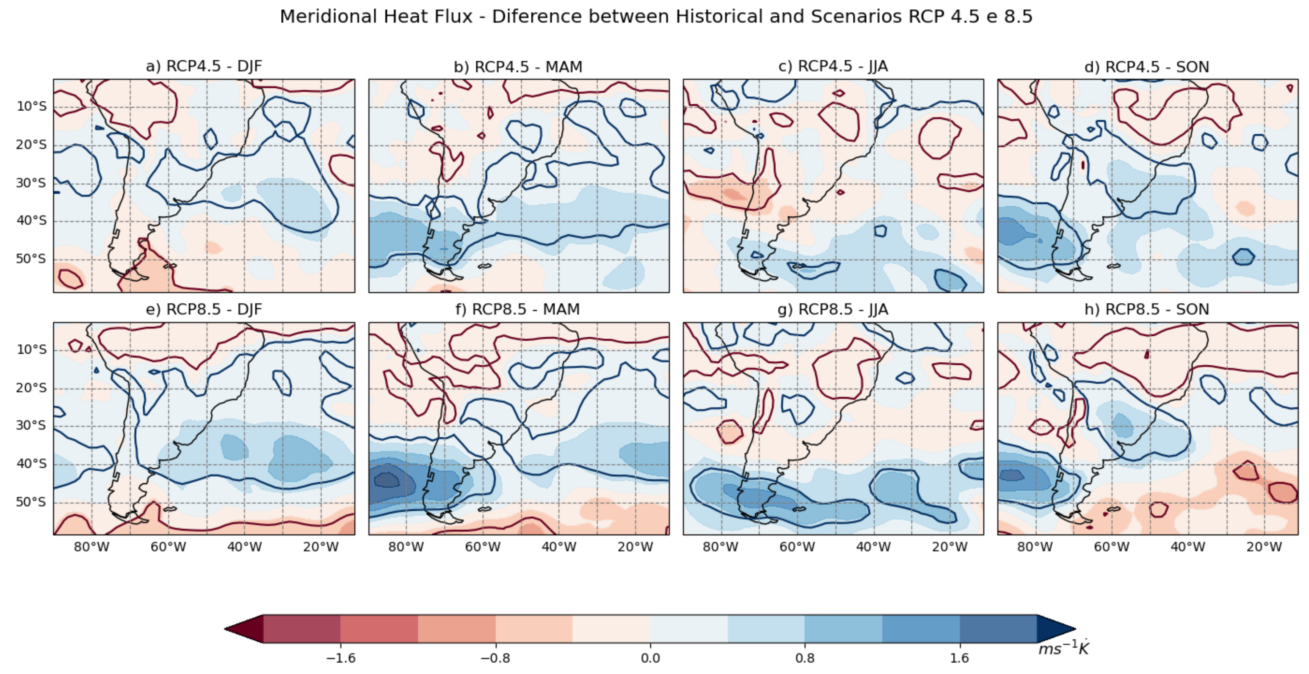
2.4.3. Meridional Heat Flux

The MHF was calculated using
M H F = v T ¯ .
It is important to highlight that v T represents the exchange between the basic state potential energy and the potential energy available for disturbances; here, u v ¯ characterizes the exchange between the KE of the disturbances and the KE of the basic state (Carmo, 2004 [32]).

3. Results

3.1. ERA5–BESM Comparison

To better understand the results, it is valid to reinforce the idea that BI and MHF have negative signals, meaning that larger values are more negative, while KE is read as usual.

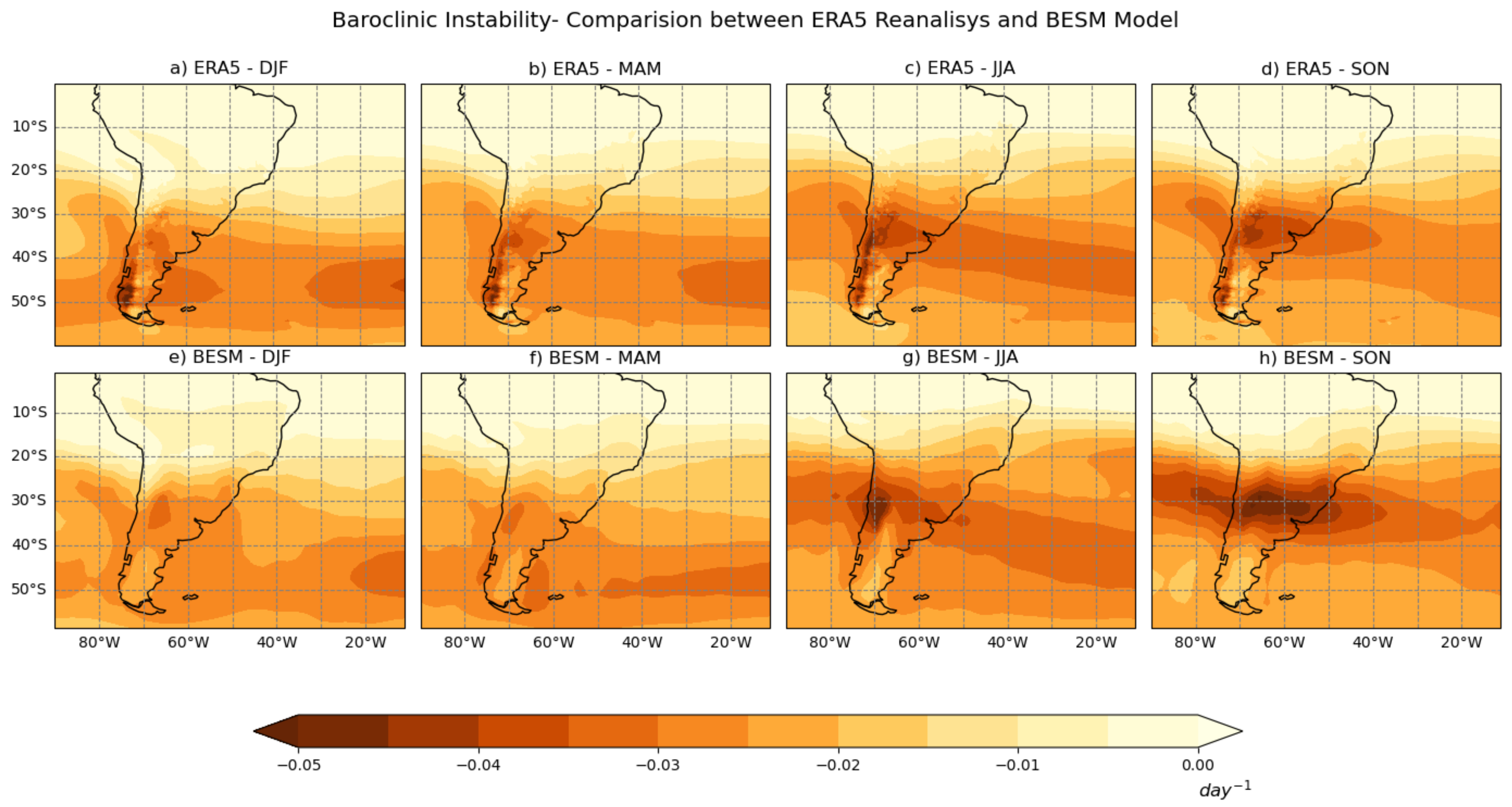
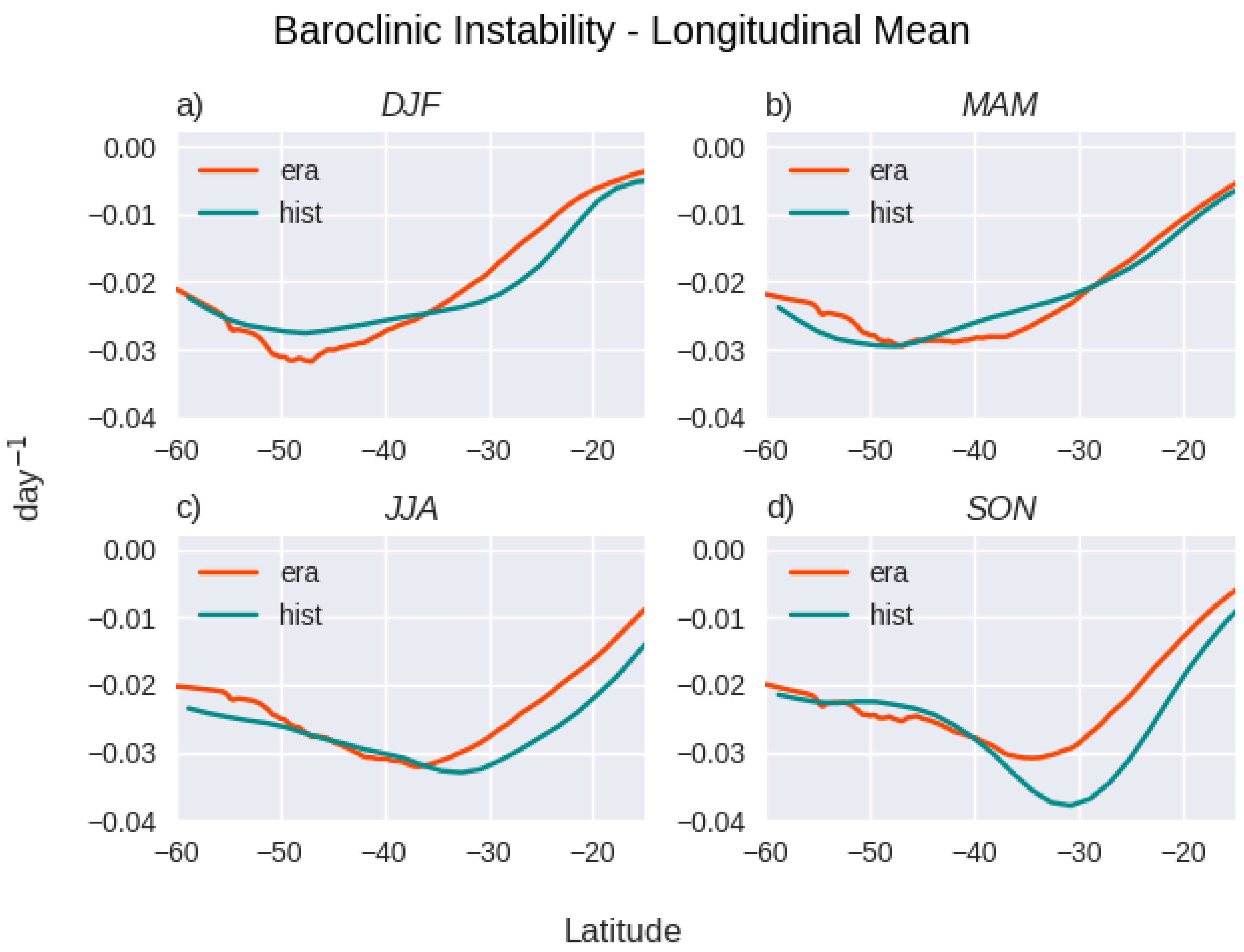
3.1.1. Baroclinic Instability

In the summer season (Figure 1a), ERA5 shows a BI track with values of −0.025 day 1 . This track covers the area above 35 to 55 ° S. The BESM model (Figure 1e) shows a similar pattern, though with more variation in the intensity on the area. Between the longitudes of 0 ° and 33 ° W and 40 ° S to 52 ° S, the baroclinicity value increases to 0.030 , with a higher intensity ( 0.035 ) near 45 ° S and at 0 to 4 ° W. In the east of the figure, there is a region with larger numbers in the south and southeast of South America extending to the ocean. The BESM model shows this increase in BI, but with a smaller longitudinal extension without this region of higher intensity and with an area of smaller values ( 0.025 ) in the south of South America (Argentina and Chile).
In the autumn (MAM), cyclogenesis is represented in the south of South America, while in the west of South America there is a region of intense baroclinicity over the whole region of Chile that is not represented by the BESM model. The ERA-MAM image (Figure 1b) shows a very similar feature to the ERA-DJF, though with lower values over the east coast in the south of South America. In the BESM model on MAM (Figure 1f), there are a number of relevant difference compared with the ERA-MAM. The region with the maxima BI is a narrowed and longer strip; on the ERA5, it covers from 40 ° S to 50 ° S and from 10 ° W to 30 ° W, while in the BESM it covers the area from 45 ° S to 50 ° S and from 10 ° W to 50 ° W. Another point of note is that the BI is reasonably high over the southwest coast of South America on the ERA, and the BESM does not show these larger values. Instead, over the east coast by Argentina there is a small region where the BESM overestimates the values of the ERA5.
In the winter (JJA), in Figure 1c,g the ERA shows a region with larger values of BI from 40 ° S to 50 ° S at 10 ° W to 30 ° S to 40 ° S at 70 ° W, with values decreasing in a westward direction. There is a similar feature in the BESM, although the area covered is from 35 ° S to 50 ° S at 10 ° W. It follows the same pattern as the ERA5, except that it stays westward. Another difference is that there is a maximal region on the coast of Chile between 25 ° S and 35 ° S that is not shown on the ERA5. In this season, the BESM overestimates the intensity of BI in this area.
For the spring season (SON) shown in Figure 1d,h, on the ERA5 (Figure 1d), the BI area, which, in JJA covers a large region of the Atlantic, is restricted to the south of South America and covers from 40 ° W to 80 ° W and from 30 ° S to 40 ° S. This area covers the land over Chile, Argentina, Uruguay, and the south of Brazil, and has a BI value of −0.035 day 1 . The BESM overestimates ERA values, providing values of −0.040 day 1 for the same area.
In Figure 2, the graphic shows the longitudinal mean of BI for the area studied (10 ° W to 90 ° ). For the summer season, Figure 2a shows that the BESM overestimates the BI from 15 ° S until nearly 40 ° S, where the BESM start to underestimate the BI until reaching 55 ° S. In autumn (Figure 2b), the BESM shows a slight overestimation, with similar values to the ERA5. From 30 ° S to 50 ° S, the BESM underestimates the BI of the ERA, and from 50 ° S to 60 ° S there is a BESM overestimation for the BI again. For the winter (figure Figure 2c), the BESM underestimates the BI from 15 ° S to 35 ° S. From 35 ° S to 50 ° S, the ERA5 and BESM values are similar, although there is a slight underestimation in the BESM values. From 50 ° S to 60 ° S, the BESM overestimates the BI. In the spring, as shown in Figure 2d, this occurs from 15 ° S to 40 ° S. From 40 ° S to 55 ° S, there is a slight underestimation of the BI, and moving southward this bias is inverted, meaning that from 55 ° S to 60 ° S there is a slight overestimation.

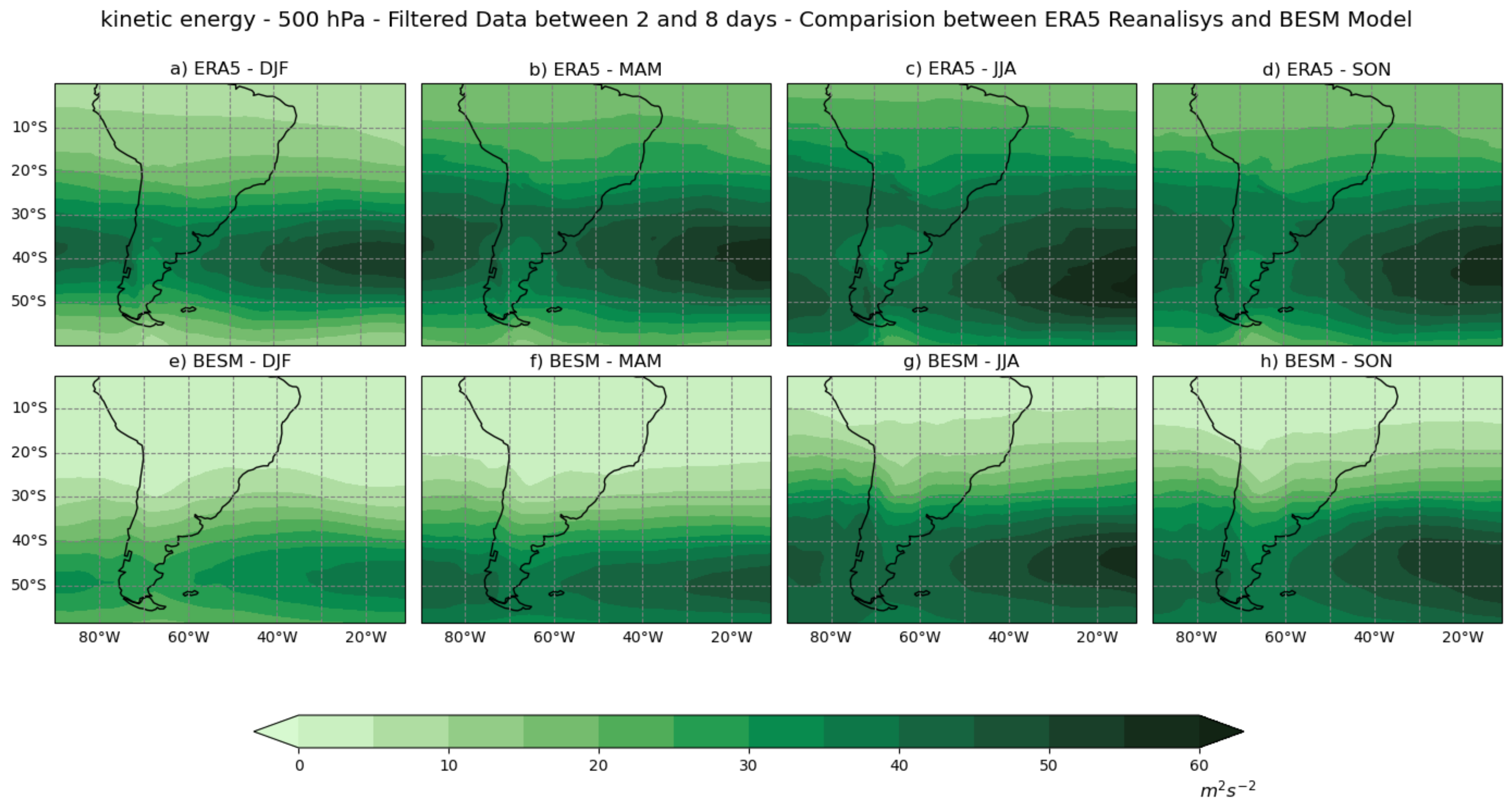
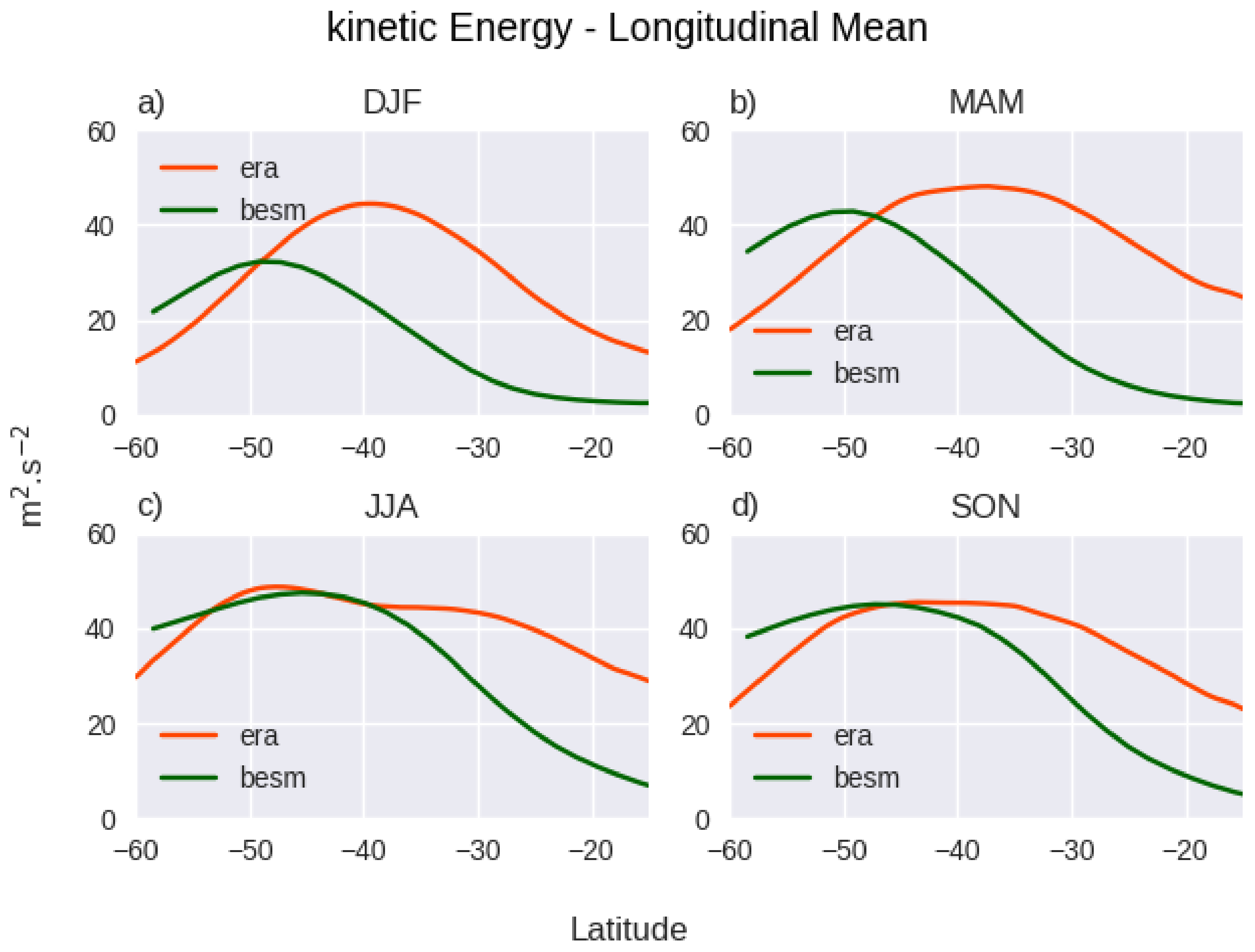
3.1.2. Kinetic Energy

In the ERA summer (DJF) dataset (Figure 3a), the maximum value of 50 m 2 s 2 occurs on the east side of the region from 35 ° S to 45 ° S and from 10 ° W to 30 ° W. There is a negative gradient moving away from this area. There is a local maximum on the west side of the frame (45 m 2 s 2 ) at latitudes of 35 ° S to 40 ° S and longitudes of 87 ° W to 90 ° W. In this image, there is a line with a value of 10 m 2 s 2 along the latitude of 10 ° S, growing to 35 ° S at a latitude of 30 ° S. This value stays the same on the continent, and there are two maximums that were cited previously in this text. Moving southward, there is a decrease in energy reaching a value of 15 m 2 s 2 at 60 ° S. In the BESM image (Figure 3e), there are smaller values of kinetic energy. In summer, there are larger differences compared to all other seasons. The east side maximum is 35 m 2 s 2 from 42 ° S to 52 ° S and from 10 ° W to 33 ° W. On the west side, the maximum value is 30 m 2 s 2 2 in the region of 46 ° S to 51 ° S and from 80 ° W to 90 ° W. The northern limit does not capture values of KE; these start at a latitude of nearly 25 ° S, with values of 5 m 2 s 2 growing to 25 m 2 s 2 near 40 ° S, where there is a maximal area.
On the ERA5 autumn (MAM) image (Figure 3b), at the latitude of 10 ° S the KE value is 20 m 2 s 2 . This value grows to 40 m 2 s 2 at the latitude of 25 ° S before increasing toward the borders, with a maximum of 55 m 2 s 2 in the region from 35 ° S to 45 ° S and 10 ° W to 23 ° W (the east side of the map), and is 50 m 2 s 2 in the region from 35 ° S to 38 ° S and 86 ° W to 90 ° W. These values decrease in the center direction as well as northward and southward. From the latitude of 80 ° S to 90 ° S, the KE decreases from 40 to 20 m 2 s 2 . The BESM dataset (Figure 3f) shows no KE northward on the map until the latitude of 20 ° S, where there is a value of 5 m 2 s 2 . This value increases to 35 m 2 s 2 at 20 ° S. The maximum value is 45 m 2 s 2 in the regions from 45 ° S to 55 ° S and 10 ° W to 30 ° W and from 43 ° S to 53 ° S and 73 ° W to 90 ° W. From the latitude of 60 ° S southward in South America, there are values of 35 m 2 s 2 . The maximum is located approximately 10 degrees southward, and there is a difference of 10 m 2 s 2 between the maximums on both sides.
The winter season (JJA), shown in Figure 3c,g, is the most similar to the region of maximum KE. On the ERA5 image (Figure 3c), there is a line of 25 m 2 s 2 at approximately 5 ° S. These values increases to 40 m 2 s 2 in the range of 25 ° S, and extend to approximately 55 ° S in this latitude range. There is a maximum on both sides. On the east side, there is a maximum of 60 m 2 s 2 from 43 ° S to 50 ° S and 10 ° W to 15 ° W, and on the west side of the map there is a maximum of 45 m 2 s 2 in the area from 43 ° S to 55 ° S and from 80 ° W to 90 ° W. The values of KE then start to decrease. On the BESM image (Figure 3g), there is a value of 5 m 2 s 2 at a latitude of nearly 10 ° S. This value increases to 40 m 2 s 2 at the latitude of 35 ° S. On the west side, there is a maximum value of 45 m 2 s 2 in the area from 40 ° S to 50 ° S and 82 ° W to 90 ° W, while on the east side there is a maximum from 40 ° S to 48 ° S and 10 ° W to 20 ° W.
In the ERA5 dataset for the spring season (SON), as shown in Figure 3d, at the latitude of 40 ° S, there is a line of 20 m 2 s 2 . This value increases to 35 m 2 s 2 at nearly 35 ° S. The east side maximum value is 55 m 2 s 2 , which occurs in the area from 37 ° S to 47 ° S and 10 ° W to 20 ° W. This value decreases to 40 m 2 s 2 on the east coast of South America. The western maximum can be seen at latitudes from 30 ° S to 47 ° S and 70 ° W to 90 ° W, with a value of 40 m 2 s 2 . This value diminishes on the west coast of South America. On the layer between 50 ° S and 60 ° S, the KE decreases from 35 to 25 m 2 s 2 . The BESM results (Figure 3h) at approximately 15 ° S show a line with values of 5 m 2 s 2 that grow to 30 m 2 s 2 when moving to 30 ° S. The east side maximum is 50 m 2 s 2 at 53 ° S and from 10 ° W to 35 ° W, which decreases to 40 m 2 s 2 near the east coast of South America. The western maximum value is 40 m 2 s 2 from 43 ° S to 57 ° S and 73 ° W to 90 ° W, stopping in Chile.
The KE longitudinal mean (Figure 4) for summer (Figure 4a) in the BESM has a lower intensity than that in the ERA5. The maximum mean value in the BESM is about 30 m 2 s 2 at 50 ° S, while that of the ERA is about 45 m 2 s 2 at 40 ° S. Locally, the BESM underestimates KE values from 15 ° S to 50 ° S. From 50 ° S to 60 ° S, the BESM overestimates the ERA values. Figure 4b shows the autumn season; in this season the BESM underestimates KE from 15 ° S to 45 ° S, while from 45 ° S and southward the BESM overestimates KE values. For the winter season (Figure 4c), the BESM underestimates the KE values from 15 ° S to 40 ° S, as in the previous seasons. From 40 ° S to 45 ° S, the BESM and ERA present the same values for KE, while from 45 ° S to 55 ° S the BESM slightly underestimates KE. From 55 ° S to 60 ° S, there is a change and the BESM overestimates the ERA5 KE values. In the spring, the BESM underestimates ERA5 from 15 ° S to 45 ° S and overestimates it from 45 ° S to 60 ° S. The largest KE values are similar in both methods, at approximately 45 m 2 s 2 .

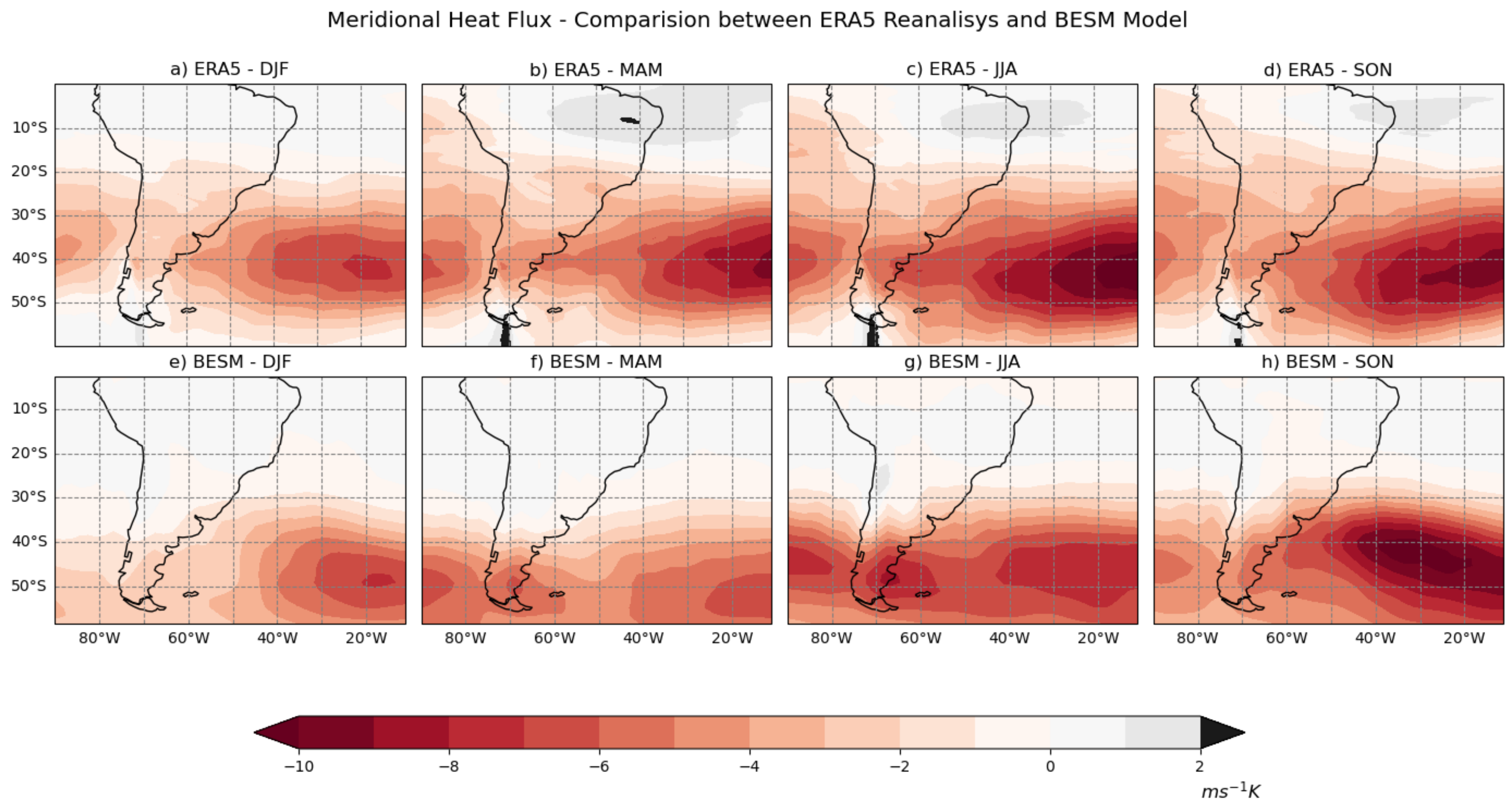
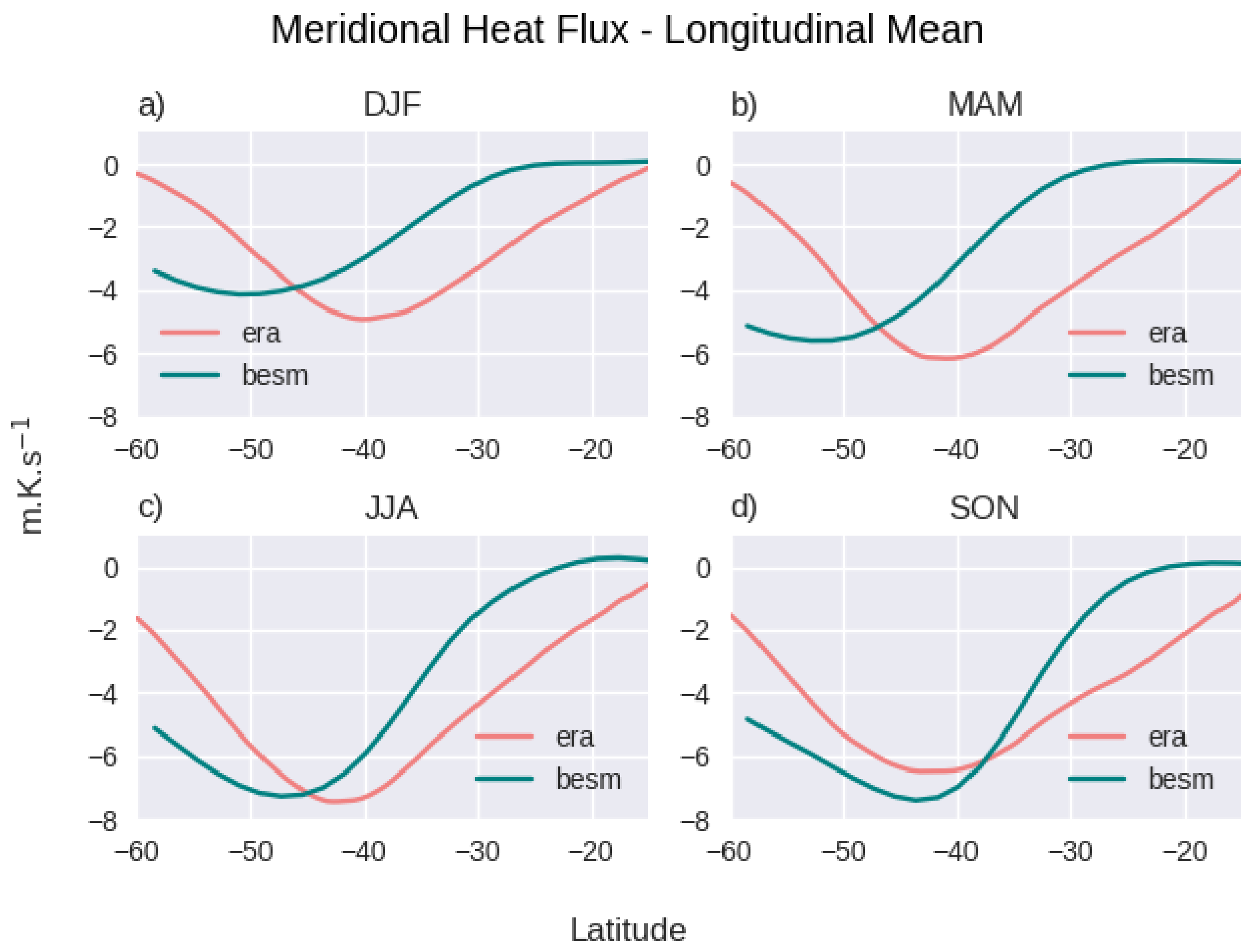
3.1.3. Meridional Heat Flux

For the summer (DJF), as presented in Figure 5a, in the region between 10 ° S and 20 ° S the MHF value is 0 Kms 1 . This value grows to −2 Kms 1 in the area from 20 ° S to 30 ° S. The west maximum value is −6 Kms 1 for the region from 37 ° S to 43 ° S and 87 ° W to 90 ° W. This value decreases to −4 Kms 1 on the west coast of South America. On the east side of the map, the maximum value is −9 Kms 1 in the region from 37 ° S to 43 ° S and 10 ° W to 15 ° W, and decreases to −3 Kms 1 on the east coast of South America. From the region between 50 ° S and 60 ° , the southward heat flux decreases from −2 to 0 Kms 1 . The BESM model (Figure 5e) shows a value of 0 Kms 1 in a wavy pattern that stays in the range of 10 ° S to 30 ° S, and the value increases to −2 Kms 1 , remains wavy, and remains from 30 ° S to 50 ° S. There is no western maximum, and the east has a maximum value of −7 Kms 1 and stays above the area from 45 ° S to 50 ° S and 10 ° W to 20 ° W. This value decreases to −3 Kms 1 adjacent to the east coast of South America.
In the ERA5 for autumn (MAM), as shown in Figure 5b, there is a northward heat flux in the northeast of Brazil with values of +2 Kms 1 , followed by a layer without significant heat flux, then a southward heat flux with a value of −1 Kms 1 in the northwest of South America that extends southward while bypassing the center of Brazil and remaining at the latitude of 20 ° S. This value increases to −3 Kms 1 from 20 ° S to 30 ° S. The western maximum (−6 Kms 1 ) is located in the region from 36 ° S to 43 ° S and 87 ° W to 90 ° W. This value decreases to −4 Kms 1 near the west coast of South America. On the east side of the map, the maximum is −9 Kms 1 in the same latitude range as the west maximum, though above 10 ° W to 15 ° W, decreases to −3 Kms 1 in the area that covers the southern part of South America, and moves in the direction of the other maximum. Below, the value decreases to −1 Kms 1 at the latitude of 60 ° S. The BESM dataset (Figure 5f) does not have positive values (northward heat flux), and the rate of 0 Kms 1 , as in the summer image, is wavy and stays above the layer between 20 ° S and 33 ° S. This value increases to −4 at around 40 ° S. The west maximum value stays just under this layer, at 45 ° S to 55 ° S and 83 ° W to 90 ° W. The maximum on the east side is −6 Kms 1 from 47 ° S to 58 ° S and 10 ° W to 17 ° W, and decreases westward.
In the ERA5 (JJA) for winter shown in Figure 5f there is a northward trend in the northeast of Brazil, with a value of +1 Kms 1 and with a smaller size. The zero line starts above the northern region of South America, moves down, and remains eastward near to the latitude of 15 ° S. The lines of −1 and −2 Kms 1 start in the north part of the map on the west side and move downward along the west coast of South America, and extend longitudinally near the latitudes of 18 ° S and 22 ° S. The MHF grows to −4 Kms 1 at around 30 ° S. The western maximum has −6 Kms 1 , is slightly larger than the western maximum of the ERA5 for autumn, and diminishes in the direction of South America. The east side has the largest value among the seasons (−10 Kms 1 ), and extends from 37 ° S to 48 ° S and 10 ° W to 20 ° W. This value decreases to westward and reaches a value of −5 Kms 1 above the south of South America. The MHF decreases southward, reaching −3 Kms 1 on the east side of South America and −1 Kms 1 on the west side. In the BESM for winter (Figure 5f), as for the first two seasons described above, the north part of the map is wavy. The value of 0 Kms 1 is on the layer between 20 ° S and 30 ° S. This value increases to −6 Kms 1 at 37 ° S. The west maximum is Kms 1 , and it remains in the area from 40 ° S to 48 ° S and 78 ° W to 90 ° W. The east side is more uniform; the maximum (−7 Kms 1 ) covers a bigger area (40 ° S to 50 ° S, 10 ° W to 43 ° W), and the gradient is smaller than in the other seasons. The maximum value covers almost all of this range at latitudes from 40 ° S to 50 ° S.
For spring (SON), on the ERA5 (Figure 5d) there is a northward heat flux on the northeast coast of Brazil, which covers a smaller area than in other seasons. The southward flux (−1 Kms 1 ) starts in the northwest of the map (0 ° S, 90 ° W) and extends in the southeast direction (18 ° S, 10 ° W). This value increases to −3 Kms 1 at around 20 ° S. The western maximum (-5 Kms 1 ) occurs in the region from 33 ° S to 45 ° S and 83 ° W to 90 ° W. On the east side (−9 Kms 1 ), the area from 38 ° S to 46 ° S and 10 ° W to 30 ° W is elongated, and the value decreases to −4 Kms 1 above the south of South America. In the BESM model (Figure 5h), the values for spring are very similar to those in the ERA5 in the mid-latitude area. The main difference is the direction of the eastern maximum feature, which has its shape turned in the southeast direction and has a maximum value of −10 Kms 1 in the BESM. In this season, northward of the map, the isolines are wavier than the ERA5 ones. There is no northward flux; the southward flux starts near the latitude 28 ° S, and increases south- and westward as well as eastward. The west maximum (−5 Kms 1 ) occurs from 41 ° S to 49 ° S and 80 ° W to 90 ° W. The east maximum, as cited above, is elongated and has a northwest—southeast direction covering the area from 18 ° S to 40 ° S and 38 ° W to 47 ° W, and has a strong negative gradient outside of this area.
The MHF longitudinal mean is shown in Figure 6; it can be seen that summer (Figure 6a), autumn (Figure 6b), and winter (Figure 6c) all present the same bias in that the BESM underestimates the southern MHF from nearly 15 ° S to 45 ° S, while from 450 to 60 ° S the BESM overestimates the southern MHF. The values vary; in DJF, the maximum MHF in the ERA occurs at 40 ° S, with a value of −5 Kms 1 , while in the BESM the maximum is 4 Kms 1 at 50 ° S. The MAM presents an ERA5 maximum of −6 Kms 1 at 40 ° S, while the BESM produces a value of approximately −5.5 Kms 1 at 50 ° S. For JJA, they present very similar values (7.5 Kms 1 ) in close latitude positions (ERA at 43 ° S and BESM at 47 ° S). For spring (Figure 6d), the BESM underestimates MHF values from 15 ° S to approximately 37 ° S while overestimating them from 37 ° to 60 ° S. In SON, the BESM presents the largest values of all seasons (7 Kms 1 ), and has larger values than the ERA5 (6 Kms 1 ), while both present the same location for their maximums of 45 ° S.

3.2. Comparison of Scenarios

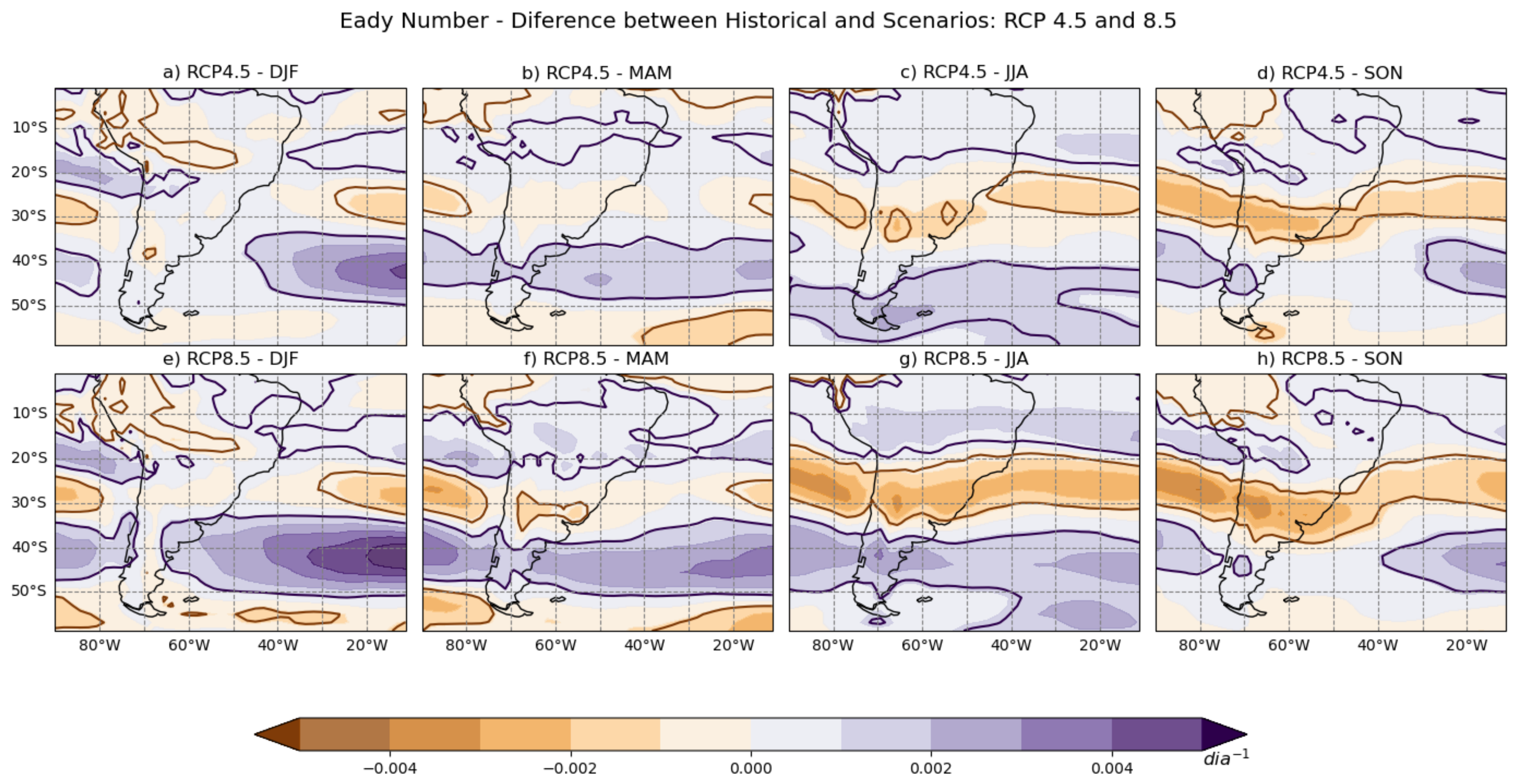
3.2.1. Baroclinic Instability

In RCP 4.5, for summer (DJF), as shown in Figure 7a, there is a reduction in the BI in the area from 34 ° S to 50 ° S and 10 ° W to 45 ° W. This reduction is more intense when the values are bigger. In the RCP 8.5 (Figure 7e) scenario, the reduction covers a bigger area (32 ° S to 50 ° S, 10 ° W to 65 ° W) and is more intense, reaching the south of South America.
In the autumn (MAM), as shown in Figure 7b,f, both scenarios present a continuous region between 34 ° S and 50 ° S with a reduction in baroclinicity. For RCP 8.5 (Figure 7e) the values are larger, leading to a larger reduction.
In winter (JJA), the RCP 4.5 scenario (Figure 7c) presents an increase in baroclinicity from 20 ° S to 30 ° S and 10 ° W to 45 ° W. There are two small areas, one above the south region of Brazil and the other above Argentina. As in the autumn, there is a layer of reduction; in this case, however, it is located southward (40 ° S to 60 ° S). In RCP 8.5 (Figure 7f), the increased area covers the whole region between 20 ° S and 30 ° S, and the reduction occurs in the same area as for the RCP 4.5 scenario, except that in this case it is more intense.
For the spring (SON), RCP 4.5 (Figure 7d) presents a region of intensification between 20 ° S and 30 ° S until 45 ° W on the southeast coast of Brazil. This layer of increase in baroclinicity continues between 28 ° S and 35 ° S and moves in the northwest direction to the west border of the map at latitudes from 20 ° S to 30 ° S. This layer is maintained in the RCP 8.5 scenario (Figure 7h), except that it is wider and has larger values. There is a decrease in baroclinicity from 35 ° S to 48 ° S and 10 ° W to 30 ° W in RCP 4.5. This decrease in values covers a larger area in the RCP 8.5 scenario (37 ° S to 50 ° S, 10 ° W to 40 ° W).

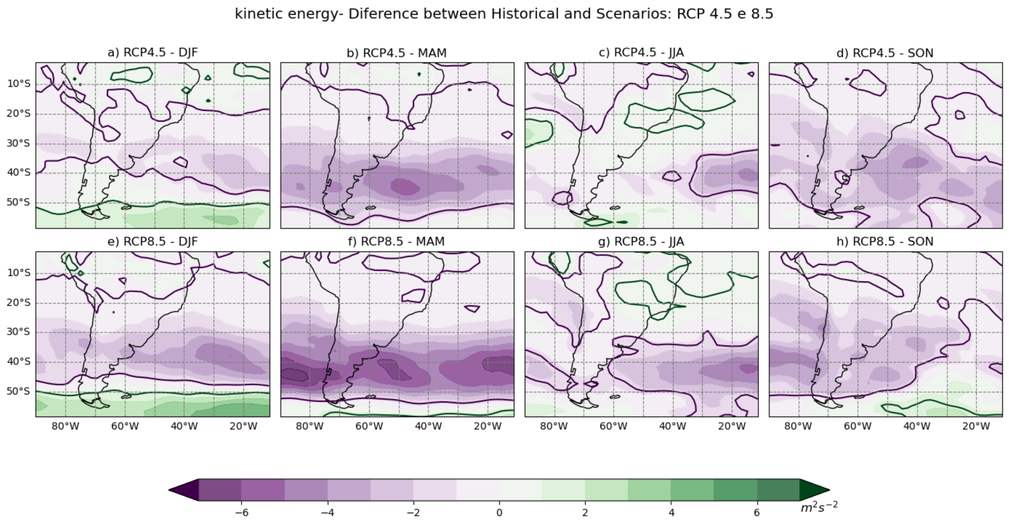
3.2.2. Kinetic Energy

For summer (DJF), in the RCP 4.5 scenario (Figure 8a) there is a decrease in KE at 500 hPa between 20 ° S and 45 ° S. The anomaly is larger on the South Brazilian coast and from 35 ° S to 45 ° S and 10 ° W to 34 ° W (−3 m 2 s 2 ). This is the same region in which there is a reduction in the BI. Below (between 50 ° S and 60 ° S) this reduction is above the same area in which there is a reduction in the BI. There is an area in which the KE increases in the layer form 50 ° S to 60 ° S, with larger values (5 m 2 s 2 ) occurring from around 30 ° W to 40 ° W. Very similar behavior is seen from 10 ° S to 47 ° S, though the reduction area is wider and the values are more negative (−5 m 2 s 2 ). The increased area occupies the same latitude layer, and the larger values (5 m 2 s 2 ) occupy a larger area, from 55 ° S to 60 ° S and 10 ° W to 38 ° W.
In autumn (MAM), as shown in Figure 8b,f, the KE in the RCP 4.5 scenario (Figure 8b) decreases throughout the whole map layer from 10 ° S to 55 ° S, with larger values (−6 Kms 1 ) near Argentina and the Uruguayan coast. For the RCP 8.5 scenario (Figure 8f), the reduction layer occupies the area from 0 ° S to 53 ° S with three maximum points: one in the extreme east of the map at around 37 ° S to 43 ° S and 10 ° W to 22 ° W, the second in the same latitude range near the south of the South American coast, and the third again at the same latitude at the extreme west the map. Almost the same situation occurs in RCP 8.5, as shown in Figure 8f; the main difference is that the reduction is larger, and there is an area with increased KE in the extreme southward part of the map.
In the RCP 4.5, for winter (JJA), as shown in Figure 8c, there is a region of decreased KE in the northeast of the map, covering the coast of the northwest part of South America as far as the northeast coast of Brazil. Down the central western part of the map from 22 ° S to 31 ° S and 80 ° W to 90 ° W and from 12 ° S to 26 ° S and 12 ° W to 26 ° W, there is a small region of increase in the south of the extreme south part of South America. On the east side of the map from 33 ° S to 48 ° S and 10 ° W to 35 ° W, there is a region of decrease in the southward heat flux. For the RCP 8.5 scenario (Figure 8g), the decrease in KE occupies three areas: the first from 0 ° S to 31 ° S and 60 ° W to 90 ° W, the second from 37 ° S to 49 ° S and 72 ° W to 90 ° W, and the third from 30 ° S to 60 ° S and 10 ° W to 60 ° W. The increased area is limited to the northeast, and is separated into two parts.
For spring (SON), in the RCP 4.5 scenario (Figure 8d) there are only neutral areas; the major part of the map is covered by decreases in KE, mainly including the area of STs. RCP 8.5 (Figure 8h) shows a major area with a reduction in KE from 0 to 50 ° S at all longitudes, and an area in the southeast (30 ° S to 60 ° S, 10 ° W to 60 ° W) of the map that is neutral from 10 ° W to 60 ° W. For spring, in the RCP 4.5 scenario only neutral areas are shown, and the major part of the map is covered by regions of decreased kinetic energy, mainly including the area of STs. RCP 8.5 has a major area covered with a reduction in KE, from 00 to 50 ° S at all longitudes, as well as an area in the southeast (20 ° S to 50 ° S, 10 ° W to 30 ° W) without significant change. Moving southward, for this neutral bias there is an area (10 ° S to 52 ° S, 55 ° W to 60 ° W) of increased KE.

3.2.3. Meridional Heat Flux

In RCP 4.5, for summer (DJF) there is a reduction in the area from 20 ° S to 40 ° S and 15 ° W to 65 ° W, as shown in Figure 9a. In the extreme south part of South America from 45 ° S to 60 ° S and 60 ° W to 72 ° W, there is an increase in southward heat flux. In RCP 8.5, the decreased area covers the area from 10 ° S to 43 ° S and 10 ° W to 70 ° W. The southward heat flux reduction occupies the whole layer from 55 ° S to 60 ° S.
In autumn (MAM), in RCP 4.5 (Figure 9b) the area of reduction in the southward heat flux is greater than in summer. It occupies an area that is wide on the east side, from 20 ° S to 40 ° S (with an appendix that goes northward), and that narrows on the coast of South America at 60 ° W, where it covers from 33 ° S to 50 ° S and extends until the end of the western side. Very similar behavior is shown for RCP 8.5 (Figure 9f), where the region of reduction starts on the east side from 15 ° S to 45 ° S, narrows at 40 ° W, and extends to the south of Brazil until 65 ° W. Southward, it covers from 33 ° S to 52 ° S, starting at 58 ° W and maintaining the reduction tendency until 90 ° W.
For RCP 4.5 for winter (JJA), as shown in Figure 9c, there are increases at dispersed points: two on the east of the map, one centered on 30 ° S, and one extended from the extreme east to 23 ° W. Northwest of this point (13 ° S to 23 ° S, 17 ° W to 28 ° W), there is another in the northeast of Brazil (9 ° S to 19 ° S, 45 ° W to 53 ° W). In the western part of South America, there is an area of higher increase from 28 ° S to 37 ° S and 65 ° W to 90 ° W. Even with the anomaly showing a larger area of reduction in the southward heat flux (at the south of the map), t-tests showed two small areas, from 53 ° S to 60 ° S and 15 ° W to 25 ° W and from 50 ° S to 55 ° S and 50 ° W to 62 ° W. For RCP 8.5 (Figure 9g), the increase in the southward heat flux occupies smaller areas in the east of the map in the northeast of Brazil. Where it occupies a larger area in western South America, the increase is smaller in this scenario and is divided into two parts. The reduction area is bigger, and is separated into three parts: an eastern one from 38 ° S to 45 ° S and 10 ° W to 17 ° W, a center one from 41 ° S to 56 ° S and 19 ° W to 41 ° W, and a larger one that covers the south of South America from 41 ° S to 58 ° S and 41 ° W to 88 ° W.
For RCP 4.5 (Figure 9d) and RCP 8.5 (Figure 9h), for spring (SON) there is very similar behavior, with two major areas of decrease in the MHF in the south and southeast regions of Brazil. This region starts on the east side (25 ° S to 38 ° S, 38 ° W) and extends northward (15 ° S, 60 ° W to 70 ° W). The other is in the southwest of the map and advances above the south of South America (33 ° S to 52 ° S, 58 ° W to 90 ° W). The main difference between the two scenarios is the size of the major region of increase in MHF over the northeast of Brazil. RCP 4.5 shows a smaller area (1 ° S to 20 ° S, 28 ° W to 60 ° W), while the RCP 8.5 scenario shows a wider one (1 ° S to 20 ° S, 28 ° W to 60 ° W).

4. Discussion

4.1. Comparison of ERA and BESM 

By observing the BI longitudinal mean (Figure 2), it is possible to see that the BESM follows the ERA5 bias, though in certain cases the BESM overestimates values and in other cases underestimates them. The largest difference occurs in SON at low latitudes, where BESM shows high BI overestimation. This can be seen on the map (Figure 1), where there is a large area over South America where this difference is notable. This can be seen in JJA as well, though to a lesser degree. The BESM underestimates the BI in DJF, MAM, and SON at medium latitudes; in this case, the largest difference is in DJF.
The BESM KE values are displaced southward in DJF, MAM, and SON, and in DJF and MAM, the values are underestimated as well, with larger differences in DJF. In JJA, the ERA presents a larger area with higher values, meaning that the KE is underestimated in this season. In the summer (Figure 3a,e) there are very similar features, except with underestimation in the southwest part of the South Atlantic and in the south of South America on both sides of the coast. Both of these regions are important for the genesis and density of extratropical cyclones, as already noted by Reboita, 2008 [36] and Gramcianinov et al., 2019 [18]. For SON, only a southward displacement is shown, with very similar values.
The ERA5 MHF presents a regular increase southward in all seasons, while the BESM presents no southward heat flux from the 0 to 30 ° S in DJF and MAM and from the 0 to 25 ° S in JJA and SON. Both the model and reanalysis show an increase in MHF followed by a decrease poleward. In DJF and MAM, the model is displaced 10 ° southward, and both underestimate the values. For KE, DJF shows the biggest difference. For winter (JJA), similar magnitudes and a 5 ° displacement are shown. The MHF values in SON present the same latitude locations in both datasets, which the BESM overestimates from 40 ° S southward.
Both the KE and MHF BESM datasets show a 10 ° displacement southward in summer and autumn in relation to the reanalysis. For the BESM, in winter and spring the areas present stronger KE and MHF values when compared with the ERA5, and they are located in the same area in both the model and reanalysis, although the BESM dataset presents a more uniform maximum area with a smaller gradient. The differences between ERA5 and BESM vary according to the season and property. For the BESM, the summer KE values are lower than the ERA5 ones, without differences in the MHF. For autumn, the BESM presents lower values in both properties for the KE and MHF. For the winter, the BESM underestimates the KE and MHF. For spring, while there is an underestimation of the KE by the BESM, the BESM overestimates the MHF.
On the wind maps Figures S1–S4, the BESM overestimates the wind magnitude, and as this value increases as the altitude increases, the differences are higher with an increased altitude, directly influencing the BI, KE, and MHF. The model presents a smaller temperature gradient at 1000 hPA (Figure S5). This could be another factor explaining the differences between the model and reanalysis.
In addition to these differences, the model reasonably represents the shape of the features. This means that the model area of the largest BI is the same as in the reanalysis, even with the difference in magnitude (which must be considered). Both the reanalysis and the model show the areas over the South American coast with biggest incidence of cyclogenesis, as already studied by Reboita et al., 2010 [21]. It is possible to see the South Atlantic region of cyclogenesis described in Gramcianinov et al., 2020 [18] as well.
In general, the Eulerian approach used in this paper has a high correlation with the Lagrangian methods used by Reboita et al. (2015) [14] and Gramcianinov et al. (2020) [18]. They mentioned an area that is separated into three, each having a different intensity of cyclone incidence throughout the year (i.e., summer and winter). This means that as it becomes colder (warmer), the maximum cyclogenesis position is more northward (southward).
It is important to observe that the calculation of the BI was conducted with mean data and the vorticity; consequently, cyclogenesis is included in the formula. On the other hand, the MHF and KE were determined with filtered data after first removing the values that were not related to extratropical cyclones. It should additionally be considered that there are differences between the model and reanalysis resolutions; these processes could interfere with the final results, as smaller features might be underestimated or even not considered at all. This difference between the methods may interfere with the forecast analysis (i.e., displacement southward in the warm seasons).
As seen in other papers, such as those by Machado et al., 2020 [15] Reboita et al., 2018, and Reboita et al., 2018 [37], the model has a lower resolution and underestimates the mean storm track areas, mainly in the warm seasons. This can be seen by comparing the graphs of MHF and KE. Another possible explanation for the summer differences between the reanalysis and the model is in relation to the SST. An EOF analysis of the BESM’s SST was conducted (Figure S2), and a discrepancy between the tendency of BESM and ERA5 was found. This may be the reason for the southward displacement of the STs on filtered data. Menendez et al. (1999) [38] analyzed the influence of the ice conditions in Antarctica under controlled conditions and their contribution to extratropical cyclones. It was verified that this coverage has high significance for the atmospheric thermodynamics, changing the balance of the transference in heat and consequently affecting this rate and modifying the ST position, as occurred in this work.

4.2. Scenarios

The BI in summer (DJF) contracts above the area of the STs. In this area, there is a reduction in KE as well. The KE is reduced in a wider area, not only in this one. The reduction covers almost all of the mid-latitude area, with a larger reduction over the STs. This whole reduction is mainly related to STs, though it is not restricted to this phenomenon. The MHF has a reduction northward of the region of the STs. In RCP 8.5, the reduction occupies a wider area, including the ST area. For RCP 8.5, the BI has the same bias as in RCP 4.5, though with higher values and over larger areas. The same occurs with the KE and MHF. An important highlight is that there is a small increase in the baroclinicity in RCP 8.5. The KE shows an increase southward of the whole map in RCP 4.5, and this increase grows in RCP 8.5. The same bias is seen for the meridional heat flux.
In MAM, in the ST zone of the RCP 4.5 BESM scenario, there is a band of decrease in BI. This reduction can be seen in KE and MHF as well; however, this diminution in KE extends for almost the whole map, while the lessening of MHF occupies almost the same band as BI. Southeast of the zone of decrease in BI, there is a zone of increase in BI, suggesting a southward relocation of the ST. Similar atmospheric behavior is seen in the RCP 8.5 BESM scenario for the same season, where the figure shows the same features plus additions, and the BI shows an increased zone southwestward on the KE map. In the extreme south, there is what can be considered the beginning of an increasing area, in agreement with the BI, although the MHF data show a disruption in the band of decrease in the MHF, suggesting the maintenance of flux in the extreme south of Brazil and north of Uruguay. There is an increase in MHF in the extreme south part of the map for KE, though only in the central region, again indicating a southward increase in the polar heat flux.
For winter (JJA), a characteristic northward ST and stronger cyclones are shown due the lower incidence of sunlight and the higher temperature gradient between the equator and pole. Both the RCP 4.5 and RCP 8.5 scenarios show the same bias, with small differences and a general intensification of the bias. The KE increases northward and decreases southward in both RCPs, with the differences being higher for RCP 8.5. The RCP 8.5 scenario presents a KE decrease southeast of the map above the same area over the ocean where there is a decrease in BI, leaving only the part on the Brazilian continent. In the extreme south of South America, there is a decrease in MHF as well. The difference in this measurement is that for RCP 4.5, on the west of the map there is a region of increase that is occupied by a neutral area, while southward of this region in RCP 8.5 there is a region that in RCP 4.5 is neutral, which becomes negative in RCP 8.5. In RCP 4.5, the MHF demonstrates small areas of decrease in the southeastern part of the map and small areas of increase in northeastern Brazil and in the west of the map, which are located southward of the region of increases in baroclinicity and KE. Both scenarios show growth in the BI, although in RCP 8.5, there is a continuous band, while in RCP 4.5 there are isolated smaller bands. Above and northward of this area there is an increase in KE and small areas of increase in MHF southward.
For spring (SON), there is an increase in the BI just above the area of the STs in the whole region between 20 ° S and 30 ° S. This behavior occurs in both scenarios, although this bias is not accomplished by the other measurements. The KE presents no variation in the east area of baroclinic increase, and decreases starting at 30 ° W; this bias is maintained westward, and occurs in both RCP 4.5 and RCP 8.5. The MHF presents a decrease above South America and in the latitude range cited above. Over this area, there is no variation in any of the scenarios. Eastward of the map, just under the region of increase of BI, there is a region of reduction in the BI in both scenarios. Above this area, the KE presents a reduction in RCP 4.5 and a neutral bias in RCP 8.5. The increase in MHF in the extreme south part of the figure is not accomplished by the other measurements. Additionally, the reduction is prevalent in the RCP 8.5 scenario.
In general, these forecasts are similar to those found in Freitas et al., 2019 [20] and Yin, 2005 [2], where there was a bias towards poleward displacement of the STs due to troposphere warming. Even with the southward displacement of the filtered data, the forecasts show a bias for displacement even more to southward. This could be part of the model in addition to the real bias that has already been described. Certain cyclones move to lower latitudes; in South America, the most important ones are formed in the Antarctic Peninsula. These cyclones contribute to mid-latitude cyclones in South Atlantic (Hoskins and Valdes, 1990 [6]). During the winter, the cyclones have longer life cycles and larger displacement compared with the summer season, and contribute more to the area studied in this paper. Another point of view is that the model presents a smaller temperature gradient in summer and a larger gradient in winter, which can shift values of BI in both cases.
Another point of view is the possibility that the atmosphere, which is under constant warming, is readapting to the new configuration; even though this paper used the last 50 years of the model’s output, the equilibrium is dynamic and the increase in greenhouse gas (GHG) emissions is predicted to grow until 2100, meaning that it is currently in the process of reaching an equilibrium. Wu et al., 2013 [39], in an experiment in which the GHGs were abruptly duplicated, concluded that a change in wind velocity alters the jet position, changing the position of the STs as well. This adaptation to new conditions may contribute to the differences between the variables analyzed here. Thus, it is necessary to study these events further using complementary methodologies and different models. One suggestion of ours is to conduct a complementary study of global models with regional models in order to better investigate these features and possible changes in them.
In general, in all seasons there is a reduction in the BI in regions of maximum values for this parameter. By analyzing the Southern Hemisphere map (Figures S6–S9),it is possible to see that this value decreases in almost all seasons in the ST region and increases southward near Antarctica. The brown lines are the contours of areas where there is a significant reduction in the BI and the purple lines are the contours of areas with significant increase, remembering that as negative values indicate more intense baroclinicity, more negative values indicate the intensification of this phenomenon.
The KE is represented in Figure 3. In general, the filtered ERA5 Figure 3a–d data have larger values than the BESM data Figure 3e–h, showing the largest differences. The smallest differences occur for JJA (Figure 3c,g), which in general has the largest values of KE. In all seasons, there are two regions of maximum KE, one on the west side of the map, with maximum values varying between 35 and 45 m 2 s 2 (30 and 45) and a latitude centered between 40 ° S and 50 ° S (50 ° S) m 2 s 2 on the ERA5 (BESM), and one on the east side, with maximum values centered at 40 ° S for all seasons except for JJA, where the maximum is centered at 45 ° S in both the reanalysis and the model. The values vary between 50 ° S and 60 ° S (35 ° S and 55 ° S) m 2 s 2 on the ERA5 (BESM). It is important to highlight that the boundaries of the image are not the same as the features, which may continue outside the limits established in this study.
In general, the BESM model (Figure 5e–h) underestimates the southward heat flux, and the maximum MHF values are located more southward than in the ERA5 reanalysis (Figure 5a–d). In addition, there is a northward flux in autumn, winter, and spring in the ERA5 in the northeast of Brazil that is not represented in the BESM. As in the KE analysis, there is a maximum on the west and another on the east side of the study field in all scenarios in the ERA5. In the BESM, for the summer scenario there is no maximum on the west side of the map. A final note concerns the transition seasons (spring and autumn), which are often not shown in other papers as they behave very similarly to the previous seasons; autumn is similar to summer and spring to winter in essentially all cases, with only slight differences.

5. Conclusions

The model presents a tendency to overestimate the BI at lower and higher latitudes, while the values for medium latitudes are either overestimated or very similar. Even though the model is capable of capturing the bias at higher and lower values, it maintains the tendencies of ERA5 with respect to BI, while for MHF and KE the model shows southward displacement compared with ERA5. In addition to these differences, the method presented here is capable of reasonably representing this genesis region using the BI, while the density distribution of cyclones across the whole study area is well represented by the KE and MHF.
The results show similar differences in both the RCP 4.5 and RCP 8.5 scenarios, with all changes being more intense in RCP 8.5. In summer and autumn, the BI decreases in the storm track areas, with KE and MHF following the propensity of BI. Winter and autumn show increased BI in the already high-intensity areas, while KE and MHF are neutral or have decreased intensity across nearly the entire region.
For better clarification of storm track locations, the use of other models might be useful. This variation could confirm or deny the BESM bias found in this paper, resulting in higher accuracy than the predictions presented herein.

Supplementary Materials

The following supporting information can be downloaded at: https://www.mdpi.com/article/10.3390/atmos14071055/s1, Figure S1: Wind speed for the level of 200 hPa (ms 1 ); seasonal comparison of ERA5 reanalysis with BESM historical data; Figure S2: Wind speed for the level of 500 hPa (ms 1 ); seasonal comparison of ERA5 reanalysis with BESM historical data; Figure S3: Wind speed for the level of 850 hPa (ms 1 ); seasonal comparison of ERA5 reanalysis with BESM historical data; Figure S4: Wind speed for the level of 925 hPa (ms 1 ); seasonal comparison of ERA5 reanalysis with BESM historical data; Figure S5: Air temperature at 1000 hPa ( ° C); seasonal comparison of ERA5 reanalysis with BESM historical data; Figure S6: Baroclinic instability in DJF (day 1 ); comparison of RCPs 4.5 and 8.5 with historical data. The lines represent the t-test and the shaded areas represent the anomalies; Figure S7: Baroclinic instability in MAM (day 1 ); comparison of RCPs 4.5 and 8.5 with historical data. The lines represent the t-test and the shaded areas represent the anomalies; Figure S8: Baroclinic instability in JJA (day 1 ); comparison of RCPs 4.5 and 8.5 with historical data. The lines represent the t-test and the shaded areas represent the anomalies; Figure S9: Baroclinic instability in SON (day 1 ); comparison of RCPs 4.5 and 8.5 with historical data. The lines represent the t-test and the shaded areas represent the anomalies.

Author Contributions

Conceptualization, J.D.D.S. and J.P.M.; methodology, J.D.D.S.; writing—original draft preparation, J.D.D.S.; writing—review and editing, J.D.D.S., J.P.M. and J.M.B.S.; funding acquisition, J.P.M. All authors have read and agreed to the published version of the manuscript.

Funding

We are grateful to Higher Education Improvement Coordination (CAPES) for providing a Master’s scholarship. We are also grateful to the National Council for Scientific and Technological Development (CNPq) for project funding (n° 406769/2021-4).

Institutional Review Board Statement

Not applicable.

Informed Consent Statement

Not applicable.

Data Availability Statement

The data used in this manuscript are available by writing to the corresponding authors.

Conflicts of Interest

The authors declare no conflict of interest.

References

  1. Peixoto, J.P.; Oort, A.H. Physics of Climate; American Institute of Physics: New York, NY, USA, 1992. [Google Scholar]
  2. Yin, J.H. The title of the cited contribution. In A Consistent Poleward Shift of the Storm Tracks in Simulations of 21st Century Climate; Geophysical Research Letters; John Wiley & Sons: Hoboken, NJ, USA, 2005; Volume 32, pp. 32–58. [Google Scholar]
  3. Blackmon, M.L.; Wallace, J.M.; Lau, N.C.; Mullen, S.L. An observational study of the Northern Hemisphere Wintertime circulation. J. Atmos. Sci. 1977, 34, 1040–1053. [Google Scholar] [CrossRef]
  4. Lau, N.C. Variability of the Observed Midlatitude Storm Tracks in Relation to Low-Frequency Changes in the Circulation Pattern. J. Atmos. Sci. 1988, 45, 2718–2743. [Google Scholar] [CrossRef]
  5. Justino, F.; Timmermann, A.; Merkel, U.; Souza, E.P. Synoptic reorganization of atmospheric flow during the last glacial maximum. J. Clim. 2005, 18, 2826–2846. [Google Scholar] [CrossRef] [Green Version]
  6. Hoskins, B.J.; Valdes, P.J. On the existence of storm-tracks. J. Atmos. Sci. 1990, 47, 1854–1864. [Google Scholar] [CrossRef]
  7. Berbery, E.H.; Vera, C.S. Characteristics of the southern hemisphere winter storm track with filtered and unfiltered data. J. Atmos. Sci. 1996, 53, 448–481. [Google Scholar] [CrossRef]
  8. Holton, J.R. An Introduction to Dynamic Meteorology; Elsevier: Amsterdam, The Netherlands, 2004; 540p. [Google Scholar]
  9. Trenberth, K.E. Storm tracks in the southern hemisphere. J. Atmos. 1991, 48, 2159–2178. [Google Scholar] [CrossRef]
  10. Leung, Y.T.; Zhou, W. Direct and indirect ENSO modulation of winter temperature over the Asian-Pacific-American region. Sci. Rep. 2016, 6, 36356. [Google Scholar] [CrossRef] [Green Version]
  11. Eichler, T.; Higgins, W. Climatology and ENSO-related variability of North American extra-tropical cyclone activity. J. Clim. 2006, 19, 2076–2093. [Google Scholar] [CrossRef]
  12. Rao, V.B.; Carmo, A.M.C.; Franchito, S.H. Interannual Variations of storm tracks in the Southern Hemisphere and their connections with the Antartic oscillation. Int. J. Climatol. 2003, 23, 1537–1545. [Google Scholar]
  13. Carmo, A.M.C.; Souza, E.B. The role of sea surface temperature anomalies on the Storm Track behavior during southern hemisphere summer. J. Coast. Res. 2009, 1, 909–912. [Google Scholar]
  14. Reboita, M.S.; da Rocha, R.P.; Ambrizzi, T.; Gouveia, D.V. Trend and teleconnection patterns in the climatology of extratropical cyclones over the Southern Hemisphere. Clim. Dyn. 2015, 45, 19–29. [Google Scholar] [CrossRef]
  15. Machado, J.P.; Justino, F.; Souza, C.D. Influence of El Niño-Southern Oscillation on baroclinic instability and storm tracks in the Southern Hemisphere. Int. J. Climatol. 2020, 41, E93–E109. [Google Scholar] [CrossRef]
  16. Machado, J.P.; Justino, F.; Pezzi, L.P. Changes in the global heat transport and eddy mean flow interaction associated with weaker thermohaline circulation. Int. J. Climatol. 2012, 32, 2255–2270. [Google Scholar] [CrossRef]
  17. Machado, J.P.; Justino, F.; Pezzi, L.P. Impacts of Wind Stress Changes on the Global Heat Transport, Baroclinic Instability, and the Thermohaline Circulation. Adv. Meteorol. 2015, 2016, 2089418. [Google Scholar] [CrossRef] [Green Version]
  18. Gramcianinov, C.B.; Campos, R.M.; Guedes Soares, C.; de Camargo, R. Analysis of Atlantic extratropical storm tracks characteristics in 41 years of ERA5 and CFSR/CFSv2 databases. Ocean. Eng. 2020, 216, 108111. [Google Scholar] [CrossRef]
  19. Gramcianinov, C.B.; Campos, R.M.; Guedes Soares, C.; Camargo, R. Extreme waves generated by cyclonic winds in the western portion of the South Atlantic Ocean. Ocean. Eng. 2020, 212, 107745. [Google Scholar] [CrossRef]
  20. Freitas, R.A.P.; Casagrande, F.; Lindemann, D.S.; Machado, J.P.; Rodrigues, J.M.; Justino, F.B. Influence of the anthropogenic effect on the dominant patterns of extratropical cyclones activity in the Southern Hemisphere. IConjecturas 2020. [Google Scholar]
  21. Reboita, M.S. South Atlantic Ocean Cyclogenesis Climatology Simulated by Regional Climate Model (RegCM3); Springer: Berlin/Heidelberg, Germany, 2009; Volume 35, pp. 1331–1347. [Google Scholar]
  22. Pezzi, L.P.; Souza, R.B.; Lentini, C.A.D. Variabilidade de mesoescala e interação oceano-atmosfera no Atlântico Sudoeste. Tempo E Clima No Bras. 2009, 1, 385–405. [Google Scholar]
  23. Hersbach, H.; Bell, B.; Berrisford, P.; Hirahara, S.; Horányi, A.; Muñoz-Sabater, J.; Nicolas, J.; Peubey, C.; Radu, R.; Schepers, D.; et al. The ERA5 global reanalysis. Q. J. R. Meteorol. Soc. 2020, 146, 1999–2049. [Google Scholar] [CrossRef]
  24. Veiga, S.F.; Nobre, P.; Giarolla, E.; Capistrano, V.; Baptista, M., Jr.; Marquez, A.L.; Figueroa, S.N.; Bonatti, J.P.; Kubota, P.; Nobre, C.A. The Brazilian Earth System Model ocean–atmosphere (BESM-OA) version 2.5: Evaluation of its CMIP5 historical simulation. Geosci. Model Dev. 2019, 12, 1613–1642. [Google Scholar] [CrossRef] [Green Version]
  25. Figueroa, S.N.; Bonatti, J.P.; Kubota, P.Y.; Grell, G.A.; Morrison, H.; Barros, S.R.M.; Fernandez, J.P.R.; Ramirez, E.; Siqueira, L.; Luzia, G.; et al. The Brazilian global atmospheric model (BAM): Performance for tropical rainfall forecasting and sensitivity to convective scheme and horizontal resolution. Weather Forecast. 2016, 31, 1547–1572. [Google Scholar] [CrossRef]
  26. Nobre, P.; Siqueira, L.S.P.; de Almeida, R.A.F.; Malagutti, M.; Giarolla, E.; Castelão, G.P.; Bottino, M.J.; Kubota, P.; Figueroa, S.N.; Costa, M.C.; et al. Climate simulation and change in the Brazilian climate model. J. Clim. 2013, 26, 6716–6732. [Google Scholar] [CrossRef]
  27. Griffies, S.M.; Schmidt, M.; Herzfeld, M. Elements of MOM4P1; GFDL Ocean Group Technical Report No. 6; Geophysical Fluid Dynamics Laboratory: Princeton, NJ, USA, 2009. [Google Scholar]
  28. Blackmon, M.L. A Climatological Spectral Study of the 500 mb Geopotencial Height of Northern Hemisphere. J. Atmos. Sci. 1976, 1602–1623. [Google Scholar]
  29. Simmonds, I.; Lim, E.P. Biases in the calculations of Southern Hemisphere mean baroclinic eddy growth rate. Geophys. Res. Lett. 2009, 36. [Google Scholar] [CrossRef]
  30. Lindzen, R.S.; Farrell, B. A Simparticlele Approximate Result for the Maximum Growth Rate of BarocliniBaroclinic instabilityc Instabilities. J. Atmos. Sci. 1980, 37, 1648–1654. [Google Scholar] [CrossRef]
  31. Paciorek, C.J.; Risbey, J.S.; Ventura, V.; Rosen, R.D. Multiple indices of Northern Hemisphere cyclone activity, winters 1949–99. J. Clim. 2002, 15, 1573–1590. [Google Scholar] [CrossRef]
  32. Carmo, A.C.M. Os Storm Tracks No Hemisferio Sul. Ph.D. Thesis, Instituto Nacional de Pesquisas Espaciais, Sao Paulo, Brazil, 2004. [Google Scholar]
  33. Wilks, D.S. Statistical Methods in the Atmospheric Sciences; Academic Press: Cambridge, MA, USA, 2005. [Google Scholar]
  34. Dal Piva, E.; Gan, M.A.; Rao, V.B. An objective study of 500-hPa moving troughs in the Southern Hemisphere. Mon. Weather Rev. 2008, 136, 2186–2200. [Google Scholar] [CrossRef] [Green Version]
  35. Raupp, C.F.M.; da Silva Dias, P.L.; da Silva Dias, M.A.F. Estudo de caso de um sistema convectivo ocorrido próximo à costa leste do nordeste do Brasil. In Proceedings of the Anais do XIII Congresso Brasileiro de Meteorologia; SBMET: Rio de Janeiro, Brazil, 2004. [Google Scholar]
  36. Reboita, M.S. Ciclones Extratropicais sobre o Atlântico Sul: Simulação Climática e Experimentos de Sensibilidade, 3rd ed.; Universidade de São Paulo: São Paulo, Brazil, 2008; pp. 154–196. [Google Scholar]
  37. Reboita, M.S.; da Rocha, R.P.; Souza, M.R.; Llopart, M. Extratropical cyclones over the Southwestern South Atlantic Ocean: HadGEM2-ES and RegCM4 projections. Int. J. Climatol. 2018, 38, 1–14. [Google Scholar] [CrossRef]
  38. Menéndez, C.G.; Serafini, H.; Le Treut, H. The Storm Tracks and the Energy Cycle of the Southern Hemisphere: Sensitivity to sea-ice boundary conditions. Ann. Geophys. 1999, 17, 1478–1492. [Google Scholar] [CrossRef]
  39. Wu, Y.; Seager, R.; Ting, M.; Naik, N.; Shaw, T.A. Atmospheric Circulation Response to an Instantaneous Doubling of Carbon Dioxide. Part I: Model Experiments and Transient Thermal Response in the Troposphere. J. Clim. 2012, 25, 2862–2879. [Google Scholar] [CrossRef] [Green Version]
Figure 1. Baroclinic instability; comparison between ERA5 reanalysis and the BESM model in day 1 . (a) ERA5—DJF (b) ERA5—MAM (c) ERA5—JJA (d) ERA5—SON (e) BESM historical—DJF (f) BESM historical—MAM (g) BESM historical—JJA (h) BESM historical—SON.
Atmosphere 14 01055 g001
Figure 2. Baroclinic instability; comparison between ERA5 reanalysis and the BESM model—longitudinal mean area. The orange line represents the ERA5 reanalysis and the blue line represents the historical scenario of the BESM model. (a) DJF (b) MAM (c) JJA (d) SON.
Atmosphere 14 01055 g002
Figure 3. Kinetic energy (m 2 s 2 ); comparison between ERA5 reanalysis and the BESM model. (a) ERA5—DJF (b) ERA5—MAM (c) ERA5—JJA (d) ERA5—SON (e) BESM historical—DJF (f) BESM historical—MAM (g) BESM historical—JJA (h) BESM historical—SON.
Atmosphere 14 01055 g003
Figure 4. Kinetic energy (m 2 s 2 ); comparison between ERA5 reanalysis and the BESM model—longitudinal mean area. The orange line represents the ERA5 reanalysis and the green line represents the historical scenario of the BESM model. (a) DJF (b) MAM (c) JJA (d) SON.
Atmosphere 14 01055 g004
Figure 5. Meridional Heat Flux (Kms 1 ); comparison between ERA5 Reanalysis and the BESM model. (a) ERA5—DJF (b) ERA5—MAM (c) ERA5—JJA (d) ERA5—SON (e) BESM historical—DJF (f) BESM historical—MAM (g) BESM historical—JJA (h) BESM historical—SON.
Atmosphere 14 01055 g005
Figure 6. Meridional heat flux (Kms 1 ); comparison between ERA5 reanalysis and the BESM model—longitudinal mean area. The light pink line represents the ERA5 reanalysis and the blue line represents the historical scenario of the BESM model. (a) DJF (b) MAM (c) JJA (d) SON.
Atmosphere 14 01055 g006
Figure 7. Baroclinic instability; comparison of RCPs 4.5 and 8.5 with historical data. The lines represent the t-test and the shaded areas represent the anomalies. (a) RCP 4.5—DJF (b) RCP 4.5—MAM (c) RCP 4.5—JJA (d) RCP 4.5—SON (e) RCP 8.5—DJF (f) RCP 8.5—MAM (g) RCP 8.5—JJA (h) RCP 8.5—SON.
Atmosphere 14 01055 g007
Figure 8. Kinetic energy; comparison of RCPs 4.5 and 8.5 with historical data. The lines represent the t-test and the shaded areas represent the anomalies. (a) RCP 4.5—DJF (b) RCP 4.5—MAM (c) RCP 4.5—JJA (d) RCP 4.5—SON (e) RCP 8.5—DJF (f) RCP 8.5—MAM (g) RCP 8.5—JJA (h) RCP 8.5—SON.
Atmosphere 14 01055 g008
Figure 9. Meridional heat flux; comparison of RCPs 4.5 and 8.5 with historical data. The lines represent the t-test and the shaded areas represent the anomalies. (a) RCP 4.5—DJF (b) RCP 4.5—MAM (c) RCP 4.5—JJA (d) RCP 4.5—SON (e) RCP 8.5—DJF (f) RCP 8.5—MAM (g) RCP 8.5—JJA (h) RCP 8.5—SON.
Atmosphere 14 01055 g009
Disclaimer/Publisher’s Note: The statements, opinions and data contained in all publications are solely those of the individual author(s) and contributor(s) and not of MDPI and/or the editor(s). MDPI and/or the editor(s) disclaim responsibility for any injury to people or property resulting from any ideas, methods, instructions or products referred to in the content.

