Article

Simulating Heavy Rainfall Associated with Tropical Cyclones and Atmospheric Disturbances in Thailand Using the Coupled WRF-ROMS Model—Sensitivity Analysis of Microphysics and Cumulus Parameterization Schemes

by
Kritanai Torsri
*,
Apiwat Faikrua
,
Pattarapoom Peangta
,
Rati Sawangwattanaphaibun
,
Jakrapop Akaranee
and
Kanoksri Sarinnapakorn
Hydro-Informatics Innovation Division, Hydro-Informatics Institute, Ministry of Higher Education, Science, Research and Innovation, Bangkok 10900, Thailand
*
Author to whom correspondence should be addressed.
Atmosphere 2023, 14(10), 1574; https://doi.org/10.3390/atmos14101574
Submission received: 28 September 2023 / Accepted: 13 October 2023 / Published: 17 October 2023
(This article belongs to the Special Issue Prediction and Modeling of Extreme Weather Events)

Abstract

:
Predicting heavy rainfall events associated with Tropical Cyclones (TCs) and atmospheric disturbances in Thailand remains challenging. This study introduces a novel approach to enhance forecasting precision by utilizing the coupled Weather Research and Forecasting (WRF) and Regional Oceanic Model (ROMS), known as WRF-ROMS. We aim to identify the optimal combination of microphysics (MP) and cumulus (CU) parameterization schemes. Three CU schemes, namely, Betts-Miller-Janjic (BMJ), Grell 3D Ensemble (G3), and Kain-Fritsch (KF), along with three MP schemes, namely, Eta (ETA), Purdue Lin (LIN), and WRF Single-moment 3-class (WSM3), are selected for the sensitivity analysis. Seven instances of heavy (35.1–90.0 mm) to violent (>90.1 mm) rainfall in Thailand, occurring in 2020 and associated with tropical storms and atmospheric disturbances, are simulated using all possible combinations of the chosen physics schemes. The simulated rain intensities are compared against observations from the National Hydroinformatics Data Center. Performance was assessed using the probability of detection (POD), false alarm ratio (FAR), and critical success index (CSI) metrics. While the models performed well for light (0.1–10.0 mm) to moderate (10.1–35.0 mm) rainfall, forecasting heavy rainfall remained challenging. Certain parameter combinations showed promise, like BMJ and KF with LIN microphysics, but challenges persisted. Analyzing density distribution of daily rainfall, we found effective parameterizations for different sub-regions. Our findings emphasize the importance of tailored parameterizations for accurate rainfall prediction in Thailand. This customization can benefit water resource management, flood control, and disaster preparedness. Further research should expand datasets, focusing on significant heavy rainfall events and considering climate factors, for example, the Madden-Julian Oscillation (MJO) for extended-range forecasts, potentially contributing to sub-seasonal and seasonal (S2S) predictions.

1. Introduction

The precipitation process comprises several critical elements within the Earth’s atmosphere. These include the presence of atmospheric water vapor, dynamic conditions responsible for the ascent and cooling of moist air parcels, and thermal conditions that dictate whether moisture condenses into either liquid or solid forms. The intricate interplay of these factors culminates in the formation of clouds and, subsequently, the occurrence of precipitation. Each of these elements, encompassing the transport of water vapor, dynamic uplift and cooling, as well as thermal influences, constitutes indispensable components in the complex mechanism underlying atmospheric precipitation. Of notable significance in this process are atmospheric disturbances and tropical storms. These meteorological phenomena exert a profound influence on the precipitation process, often resulting in heavy rainfall events. Their impact stems from their unique ability to transport moisture, instigate upward vertical motion, establish convergence zones, interact with local topography, exhibit prolonged durations, release substantial energy, and thrive under conditions of atmospheric instability. Notably, tropical storms find their genesis in the highly energetic conditions prevailing over warm tropical oceans [1]. The warming of oceanic waters plays a pivotal role in cyclogenesis, as well as the subsequent intensification of tropical cyclones. This intensification is influenced by various factors, including the intensity of steering flows, the positioning of cyclonic circulation, atmospheric stability, and wind shear conditions [2,3,4].
The Indochina Peninsula (IP) is geographically located in Southeast Asia, making it prone to tropical storms and typhoons. The region is influenced by the South China Sea (SCS) and the Bay of Bengal (BoB), recognized as breeding grounds for tropical cyclones [5,6,7]. The SCS exhibits elevated frequencies of tropical storms due to the presence of low-level cyclonic circulation and their westward propagation toward the BoB. Consequently, this movement significantly affects extreme rainfall events over the IP sub-region during the late rainy season [8,9]. The IP generally experiences a tropical cyclone season from May to November, with peak activity concentrated between July and October, resulting in heavy rainfall, strong winds, and potential flooding. Additionally, heavy rainfall in the region can be induced by monsoon depressions along the monsoon trough. The frequency and intensity of tropical storms vary annually, influenced by regional and global climate patterns, including the El Niño-Southern Oscillation (ENSO), sea surface temperatures (SST), and atmospheric conditions [10].
Thailand, located centrally within the IP region, has consistently experienced severe and devastating flooding events on an interannual basis, primarily due to heavy rainfall associated with atmospheric disturbances. These events have resulted in significant socio-economic damage. Historical records reveal that catastrophic floods in Thailand have typically coincided with synoptic conditions, particularly tropical storms, renowned for their capacity to generate extreme weather, flooding, and storm surge [11,12,13,14,15]. Therefore, precise prediction of these high-impact weather events is vital for effective preparedness, early warning systems, and the implementation of disaster management strategies, which are crucial in mitigating the potential impacts of tropical storms on the region.
In recent decades, dynamic numerical forecast models have significantly advanced, effectively integrating atmospheric, surface, and subsurface processes, thereby extending the forecast period for tropical storms and flood events [16,17,18,19]. In a previous study, Islam et al. [16] utilized a dynamical model, specifically the WRF model, to simulate Typhoon Haiyan, a formidable Category-5 equivalent super typhoon. While the WRF model effectively predicted the typhoon’s trajectory, it encountered challenges in intensity forecasting, highlighting the need for improvement. Potty et al. [17] focused on evaluating the WRF model’s forecasting capabilities for typhoons with varying trajectories, showcasing its proficiency in predicting factors such as landfall timing and mean sea-level pressure. Wu et al. [18] delved into the complex relationship between typhoons and rainfall patterns over the SCS, revealing the spatial asymmetry in typhoon-related phenomena and emphasizing intricate nonlinear interactions. Sivaprasad et al. [19] assessed the accuracy of meteorological data derived from the WRF model during Tropical Storm Pabuk’s passage over the southern SCS. While the model aligned well with buoy data before and after the storm’s passage, it encountered discrepancies during the storm, emphasizing the challenge of simulating intense meteorological conditions. These studies collectively provide valuable insights into typhoon modeling, forecasting, and their interactions with the SCS, contributing to an improved understanding and prediction of these critical weather events.
Moreover, progress in atmospheric science owes much to improved comprehension of physical processes, refined parameterizations, advanced data assimilation techniques, high-resolution observations, enhanced computational capabilities, and international collaboration [20,21,22,23,24]. There is a growing emphasis on elevating the predictive prowess of numerical weather prediction (NWP) models, especially concerning intricate atmospheric processes such as aerosol dynamics, climate phenomena, seasonal forecasting, and surface-atmosphere interactions. The prediction of aerosol particle properties, crucial for stakeholders like air quality regulators, aviation, solar energy management, and climate service providers, presents intricate challenges driven by the complex nature of aerosol processes and their sensitivity to meteorological conditions, necessitating source term accuracy, meteorological influence, and aerosol chemistry enhancements. Simultaneously, Francisco et al. [21] stressed the significance of seasonal forecasting quality evaluation, exploration of atmosphere-ocean coupling, and process-based verification to bolster forecast reliability. This drive for enhanced predictions extends to Portugal, where Monteiro et al. [22] underscored the importance of surface-atmosphere interactions, emphasizing multidimensional observational data integration and national assimilation system development. Furthermore, Linardakis et al. [23] highlighted the potential of component concurrency in the era of exascale computing, enabling better scalability and handling increasing model complexity. Meanwhile, Baklanov et al. [24] shed light on the evolution of online coupled meteorology-atmospheric chemistry models, recognizing their relevance for air quality, weather prediction, and climate research, although they present scientific challenges. In synthesizing these insights, it is clear that improving atmospheric predictions and climate projections hinges on understanding intricate relationships between meteorological processes, atmospheric composition, and the computational resources essential for effective modeling.
However, current dynamic forecast models still have limitations in efficiently predicting tropical storms and capturing the intricate interplay between complex oceanic conditions and air-sea interactions that modulate heavy rainfall on a regional scale [25,26,27]. These models entail complexity and necessitate numerous assumptions regarding cloud formation and its interaction with the atmosphere. These assumptions are typically encompassed within microphysical (MP) and cumulus (CU) parameterization schemes.
In numerical atmospheric models, the CU parameterization scheme plays a vital role in accounting for sub-grid-scale cloud-radiation interactions, which are intricately connected to the vertical redistribution of atmospheric heat and moisture tendencies [28,29]. Furthermore, the microphysical (MP) parameterization, which influences the sub-grid- scale vertical flux of cloud and sedimentation processes of hydrometeors, also plays a crucial role at the regional level [30,31]. These effects on tropical cyclone intensity, such as moisture distribution, latent heating, and convection, are critical for improving simulations during tropical storms in the surrounding areas of Thailand [32,33,34]. A microphysics scheme can also provide a better representation of evaporation processes from frozen hydrometeors and a substantial quantity of liquid hydrometeors, resulting in improved latent heat release in storms and a correlated increase in precipitation amounts and distribution [35]. The significance of CU and MP parameterization in simulating tropical storms and regional rainfall has been highlighted in previous studies [16,17,18,19,28,29,30,31,32,33,34,35]. However, it is important to note that the existing research primarily focuses on specific tropical storm events, resulting in a limited number of cases and insufficient systematic analyses regarding the temporal and spatial consistency associated with regional rainfall. Furthermore, a notable limitation of prior research lies in the exclusive reliance on atmospheric models in isolation. This approach tends to disregard the pivotal role of air-sea interaction in shaping the characteristics and behavior of tropical storms. Although atmospheric modeling retains its fundamental significance, there exists a pressing necessity to complement it with models that encompass the intricate interplay between the atmosphere and the ocean. This holistic approach is essential for a more accurate representation of the dynamics and outcomes of the tropical storm processes [36,37,38].
Based on the aforementioned considerations, it is crucial to address three key aspects when improving the model performance. These include incorporating the air-sea interaction process into the simulation, exploring the sensitivity of CU and MP parameterization for improved short-term rainfall forecasting during tropical storms, and refining the boundary and physical conditions. Consequently, the objective of this study is to investigate the relative sensitivities of various CU and MP parameterization schemes in simulating spatiotemporal variations of rainfall during tropical storm events in Thailand, utilizing the WRF-ROMS model. Specifically, this paper focuses on simulating heavy rainfall patterns in Thailand during tropical storm events at a high horizontal resolution of 3 km and examining the forecast skill associated with different CU and MP schemes.
Section 2 provides a detailed description of the model configuration and the design of sensitivity experiments conducted in this study. Section 3 outlines the methodology for selecting tropical storm events, the observational data utilized for evaluation, and the verification methods employed. In Section 4, we evaluate the forecast skill of rainfall in various regions of Thailand across four distinct rainfall categories and present a comprehensive discussion of the results. Finally, Section 5 summarizes the main findings derived from this study.

2. Materials and Methods

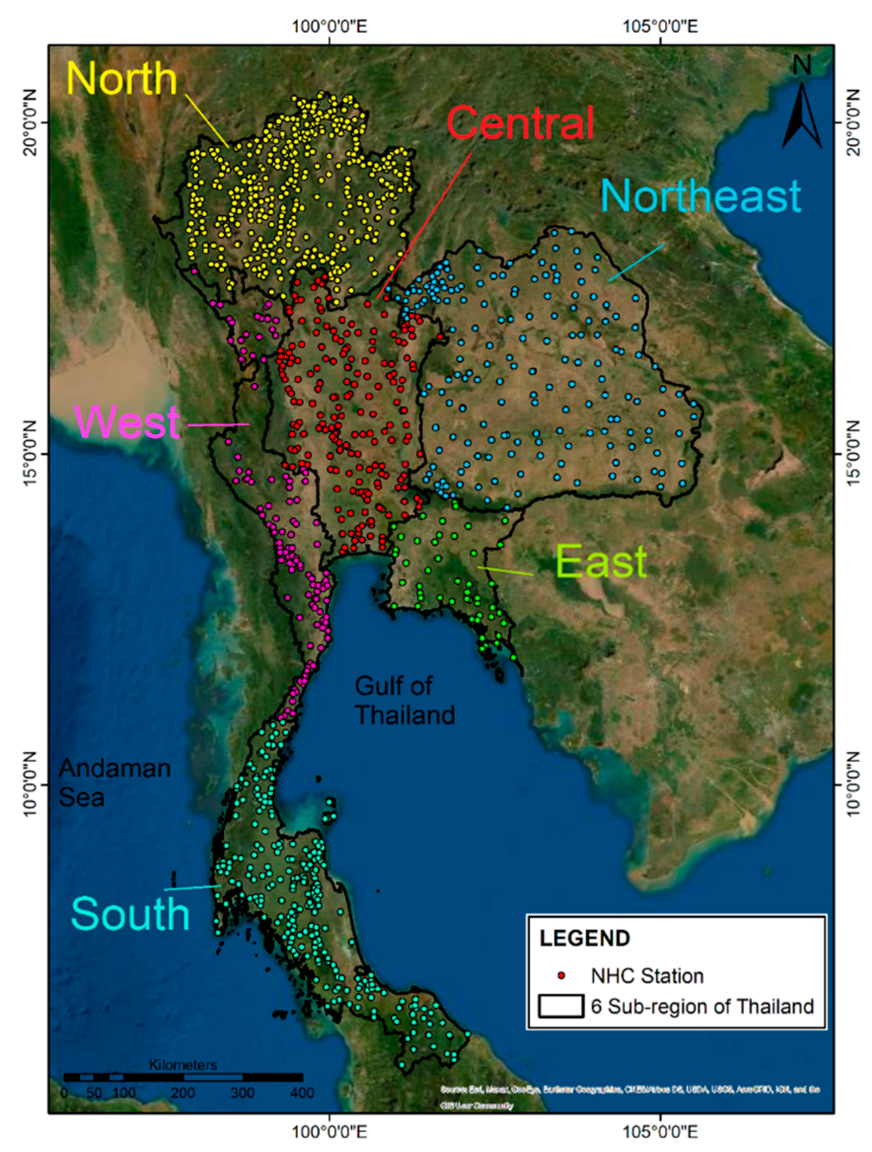
2.1. Observed Rainfall Data

For our analysis, we collected daily rainfall data from a comprehensive network of 1234 National Hydroinformatics Data Center (NHC) stations. Figure 1 shows the spatial distribution of the NHC stations utilized in this study.
These stations were distributed across different regions of Thailand, with 213 stations in the central region, 119 stations in the western region, 49 stations in the eastern region, 188 stations in the northeastern region, 422 stations in the northern region, and 243 stations in the southern region. The rainfall intensities simulated in this study were compared to observations obtained from the NHC, which serves as a pivotal repository for hydrological and meteorological data in Thailand. The NHC has emerged as a vital hub for water resource management, disaster preparedness, and scientific research by establishing data linkages with over 50 agencies (https://www.thaiwater.net/ (accessed on 27 September 2023)).

2.2. Model Configurations and Experiment Designs

2.2.1. Model Description

In this study, we employed a coupled modeling system, known as the Coupled Ocean-Atmosphere-Wave-Sediment Transport modeling system (COAWST), that originally developed at the United States Geological Survey (USGS) [37,38]. In the COAWST, interactions of different physical processes of the Earth’s components, that is, ocean, atmosphere, wave, sediment transport, and sea-ice are integrated into the modeling system. The coupled modeling system is open source, free of charge, and available online at https://code.usgs.gov/coawstmodel/COAWST (accessed on 27 September 2023).
The COAWST system utilizes the Regional Ocean Modeling System (ROMS) as a functional modeling framework to estimate the state of the ocean. ROMS is a numerical model based on a free-surface, terrain-following approach, employing hydrostatic and Boussinesq approximations [39,40]. It provides a means to simulate the ocean’s behavior and processes. Concurrently, the Weather Research and Forecasting (WRF) Model is employed to estimate atmospheric variables. WRF is an advanced mesoscale model based on a non-hydrostatic atmospheric formulation, utilizing terrain-following vertical coordinates [41]. Widely employed by the scientific community, the WRF model facilitates diverse research studies and operational applications, for instance, potential solar and wind energy resources, localized flood hazards, short-term weather forecasting, and climate studies [42,43,44,45,46,47]. It is important to acknowledge that the specific formulations and parameterizations of cumulus schemes in the WRF model may vary, with different schemes prioritizing specific tendencies. Consequently, researchers and modelers frequently calibrate these schemes using observational data to enhance their representation of real-world atmospheric processes, particularly when coupled with oceanic models.
The WRF-ROMS coupling allows for the simulation of interactions between the atmosphere and the ocean, which can be important for understanding weather patterns and their effects on oceanic processes. This model has been used in a variety of applications, including forecasting ocean conditions and predicting the impacts of storms on coastal regions. Torsri et al. [48] conducted an initial research endeavor aimed at evaluating rainfall simulation in Thailand by comparing coupled and non-coupled approaches. Their findings suggested that incorporating air-sea interaction in the modeling framework yielded superior results compared to the non-coupled approach. However, the previous study did not specifically investigate the impacts of different cumulus and microphysics options within the WRF model. Consequently, the examination of these factors remains a pertinent challenge that necessitates further investigation.
Note that the modeling system used here is the COAWST version 3.2, which is the same version being officially routinely operated at the Hydro-Informatics Institute, Ministry of Higher Education, Science, Research and Innovation, Thailand, since 2016 for the short-term weather forecast system (7 days in advance). So far, the WRF-ROMS forecasted results are publicly available online at https://www.thaiwater.net/weather/ (accessed on 15 October 2023) and also disseminated to stakeholders and researchers that related to disaster prevention, early warning, and water resource management in Thailand and some ASEAN countries (https://www.aseanwater.net/ (accessed on 27 September 2023)). This study focuses on examining synoptic weather systems and rainfall forecasts, with particular attention given to the influence of air-sea interactions. To facilitate this investigation, the WRF is coupled with the ROMS. While certain microscale processes (i.e., wave and sediment components) occurring at scales smaller than the model’s grid cells can be disregarded, other important components are considered.

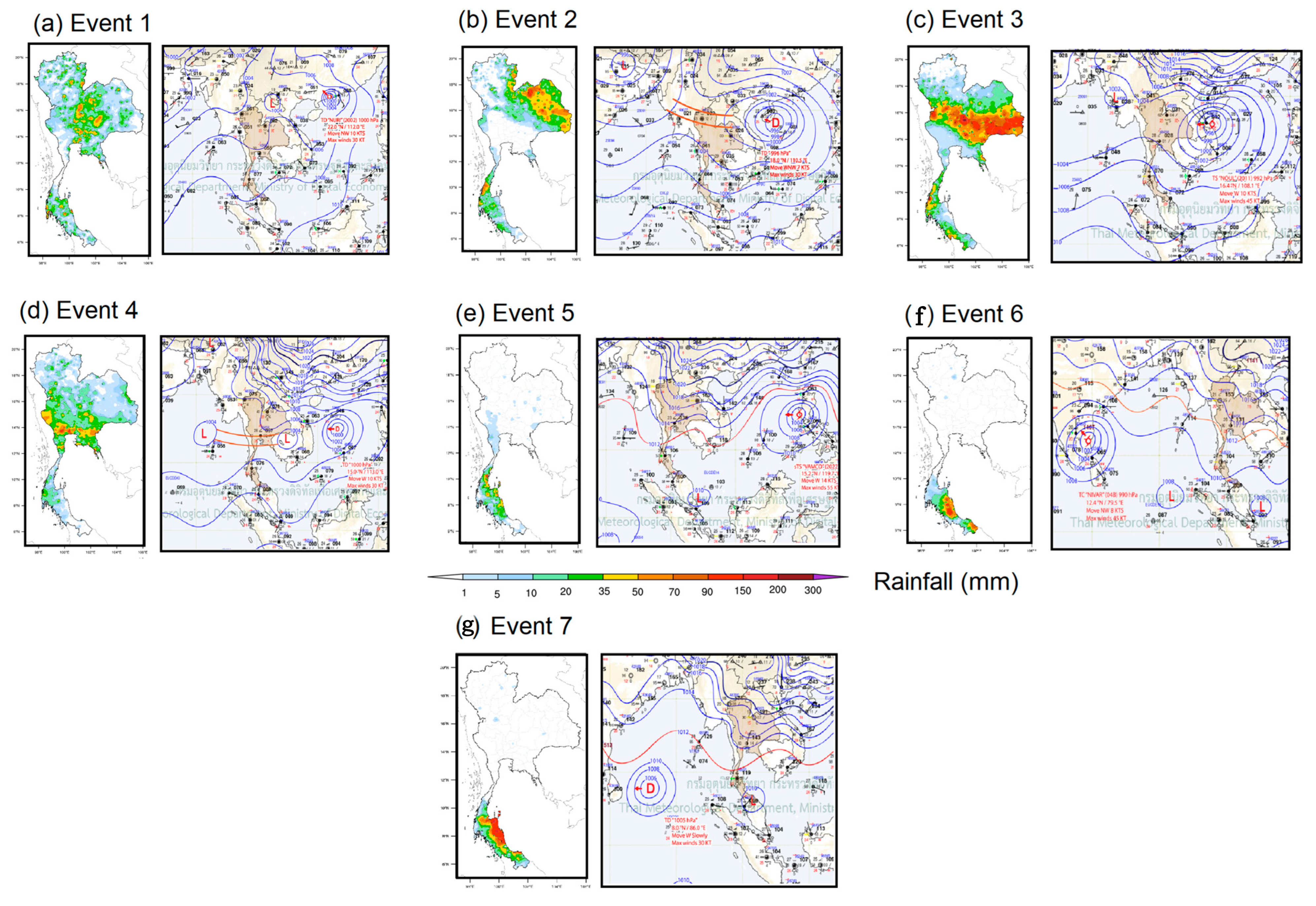
2.2.2. Selection of Heavy Rainfall Events

According to the definition given by the Thai Meteorological Department [49], daily rainfall in the region can be classified into five distinct categories: (1) trace rain (<0.1 mm), (2) light rain (0.1–10.0 mm), (3) moderate rain (10.1–35.0 mm), (4) heavy rain (35.1–90.0 mm), and (5) very heavy or violent rain (>90.0 mm). The main objective of this study is to assess the impacts of CU and MP on the estimation of high-impact weather events, specifically focusing on heavy (>35.0–90.0 mm/day) and violent rainfall (>90.0 mm/day) categories. Throughout the paper, we will consistently adhere to the TMD’s definition for our analysis and discussions.
In 2020, Thailand experienced several instances of heavy rainfall, primarily attributed to atmospheric disturbances. In this year, the weather condition of Thailand can be attributed to the significant impact of storms. These disturbances included events such as Sinlaku in August, tropical storm Noul in September, and typhoon Molave in October. These occurrences resulted in significant rainfall throughout the country, particularly in the northern regions, leading to severe damage to infrastructure, properties, and agricultural resources [47]. Apart from atmospheric disturbances, heavy rainfall in Thailand can also be caused by a low-pressure zone known as the monsoon trough. During the summer monsoon season, this trough shifts northward, resulting in heavy rainfall and wet conditions in the northern parts of Thailand. Conversely, during the winter monsoon season, the trough shifts southward, leading to drier conditions in the north and increased precipitation in southern Thailand. Hence, a selection of events that occurred during June to December in 2020 is a suitable choice for verifying prediction skills with different combinations of cumulus and microphysics options due to the following reasons: (1) variety of atmospheric disturbances that exhibited different characteristics and intensities, providing a diverse set of conditions to evaluate the prediction skill of different cumulus and microphysics options and (2) significant impact on rainfall by which the selected events resulted in substantial rainfall across Thailand.
Here, we conducted a case study focusing on seven significant heavy rainfall events that took place in 2020, each of which was associated with atmospheric disturbances (i.e., tropical storms, depressions, low pressure, and monsoon troughs). These disturbances either moved through or formed within a defined geographical area (0.0–25.0°N, 90.0°E–120.0°E), which is known to potentially impact on the weather conditions of Thailand [50]. Table 1 provides detailed information regarding each selected event. Figure 2 draws the spatial distribution of rainfall on the target date alongside its corresponding synoptic weather chart, which we used to analyze the behavior of each event.
On June 14th (Event 1), Thailand experienced heavy rainfall, particularly in the northern, northeastern, central, and eastern regions, with rain intensity reaching a maximum of 90.0 mm in certain areas. This rainfall event was caused by a tropical depression named Nuri, which originated in the eastern part of the Philippines and passed through the upper part of the SCS (Figure 2a). Subsequently, on August 1st, another notable heavy rainfall event occurred due to Tropical Depression Sinlakul (Event 2). The Sinlakul initially formed as a tropical depression over the northern SCS on the morning of July 31st. It further intensified into a tropical storm and gradually moved toward the northern regions of Vietnam over the following days. Before entering Thailand, Sinlakul weakened and transitioned into a tropical depression. As Sinlakul traversed through Thailand (on 1st August), in conjunction with the presence of the monsoon trough over the region, these combined weather conditions resulted in heavy to violent rainfall, reaching the highest intensity of about 150.0 mm, primarily in northeastern Thailand (Figure 2b). As a result, the area experienced widespread flooding, landslides, rapid water surges, forest runoff, and extensive damage to properties [47].
On September 18th (Event 3), Thailand encountered a notable increase in rainfall, characterized by heavy to very heavy rainfall in the upper sub-regions (Figure 2c). The highest recorded intensity of 243.8 mm was observed in Phetchabun Province in the north [50]. This increase in rainfall was attributed to the impact of a tropical depression that intensified into a tropical storm (TS) and was internationally named “Noul”. The storm’s trajectory moved toward northeastern Thailand, passing through the central and eastern regions and extending into certain areas of the western regions (Figure 2c). As a result, widespread flooding and flash floods occurred in multiple areas. On October 16th (Event 4), a combined effect of a tropical depression (TD) moving westward from the central SCS toward Vietnam, along with the intensified monsoon trough sweeping across the central, eastern, and upper regions of southern Thailand. This meteorological phenomenon led to substantial rainfall in these areas of Thailand, with certain locations experiencing rainfall exceeding 90.0 mm (Figure 2d).
During the latter months (November to December), corresponding to the winter season in Thailand when the northeast monsoon prevails, there was a frequent occurrence of heavy rainfall events in southern Thailand (Events 5 to 7). These events were primarily concentrated along the east coast of the south, where heavy to violent rainfall was commonly observed (refer to Figure 2e–g). These weather patterns were attributed to the formation of a low-pressure system induced by a tropical storm in the SCS, and occasionally influenced by a tropical cyclone in the BoB.
To facilitate model integration, we established three distinct initial dates for the study: the date corresponding to heavy rainfall occurrence (lead-0), the date preceding the event (lead-1), and the date further preceding the event (lead-2) (refer to Table 1 for specific information). Subsequently, we conducted model integration and simulation for a period of 24 h, 48 h, and 72 h for each of the aforementioned lead times to simulate the target date of each event. In doing this, the diverse range of atmospheric patterns observed in the selected events provides a solid foundation for evaluating the effectiveness and accuracy of different cumulus and microphysics parameterizations in predicting and capturing heavy to violent rainfall patterns across Thailand.

2.2.3. Combinations of CU and MP

It is acknowledged that the estimation of rainfall over a certain region in an atmospheric model is strongly dependent on CU and MP parameterizations. Many studies have revealed that applying different combinations of cumulus and microphysics options in a model for a region can yield different results [29,30,31,32,33,34,35,51,52]. For instance, Guo et al. [52] examined the sensitivity of the model’s performance to the choice of MP schemes and evaluated the simulations against observed data. They highlighted the performance differences among three MP parameterization options in simulating various aspects of rainfall patterns and diurnal variations, which were found to be sensitive to the choice of microphysics parameterizations.
In this study, we designed, in total, 9 combinations of CU and MP parameterizations by which three CU schemes, namely, Betts-Miller-Janjic (BMJ), Grell 3D Ensemble (G3), and Kain-Fritsch (KF) along with three MP schemes, namely, Eta Ferrier (ETA), Purdue Lin (LIN), and WRF Single-moment 3-class (WSM3), were selected for the sensitivity analysis. It is important to note that the combination of the BMJ and ETA parameterization is denoted as the control run (CTRL) in this study. The selection of this particular combination as the control run is justified by its prior verification in Torsri et al. [48], as well as its ongoing utilization within the current operational system at the Hydro-Informatics Institute, Thailand. Consequently, it serves as a reference (CTRL run) against which other combinations are compared in our analysis. A summary of combinations is given in Table 2. The seven instances of heavy to violent rainfall in Thailand (listed in Table 1), occurring during June to December of 2020 and associated with tropical storms and atmospheric disturbances, are simulated using all possible combinations of the chosen physics schemes.
The BMJ, G3, and KF schemes are widely used in atmospheric modeling and have been extensively evaluated and tested in tropical regions [59,60,61,62]. The main differences among these schemes lie in the complexity of the parameterization and the treatment of convective processes. BMJ is relatively simple, using a relaxed Arakawa-Schubert closure. G3 employs an ensemble-based approach with multiple convective plumes, while KF operates on a higher-resolution grid and includes a downdraft parameterization. Overall, while all three schemes consider the transport of moisture within cumulus convection, they may have different parameterizations for specific processes such as detrainment, entrainment, and vertical mixing for the treatment of moisture tendencies (Table 3). The assumptions made in each scheme affect how moisture tendencies are represented and contribute to the overall moisture budget within the model grid cell [63].
The choice of microphysics is of utmost importance due to its significant impact on the accurate representation of key atmospheric processes, including water vapor, cloud droplets, ice particles, rain, and other hydrometeors within the atmosphere. The precise simulation of these processes is directly linked to the reliability and accuracy of weather forecasts and simulations. In order to comprehensively evaluate the representation of interactions between cumulus convection and microphysical processes, it is essential to consider a diverse range of microphysics options in conjunction with the selected CU schemes. For this study, we have specifically chosen three MP schemes, namely, ETA, LIN, and WSM3, to describe the distinct interactions among water vapor, cloud droplets, ice particles, rain, and other hydrometeors within the atmosphere (refer to Table 3 for details).
In this study, our main objective is to predict heavy rainfall that is linked to atmospheric disturbances, with a specific emphasis on tropical regions. To achieve this goal, we have selected certain CU and MP schemes that have previously shown outstanding performance in situations characterized by tropical atmospheric disturbances and have been previously validated and found to excel in modeling such conditions [51,52,59,60,61,64,65,66]. However, it is important to note that the effectiveness of a particular combination of CU and MP options in one region does not guarantee similar performance in another region. Therefore, prior to the application of any CU and MP scheme in a specific area of interest, conducting a sensitivity analysis on the parameterization is essential.

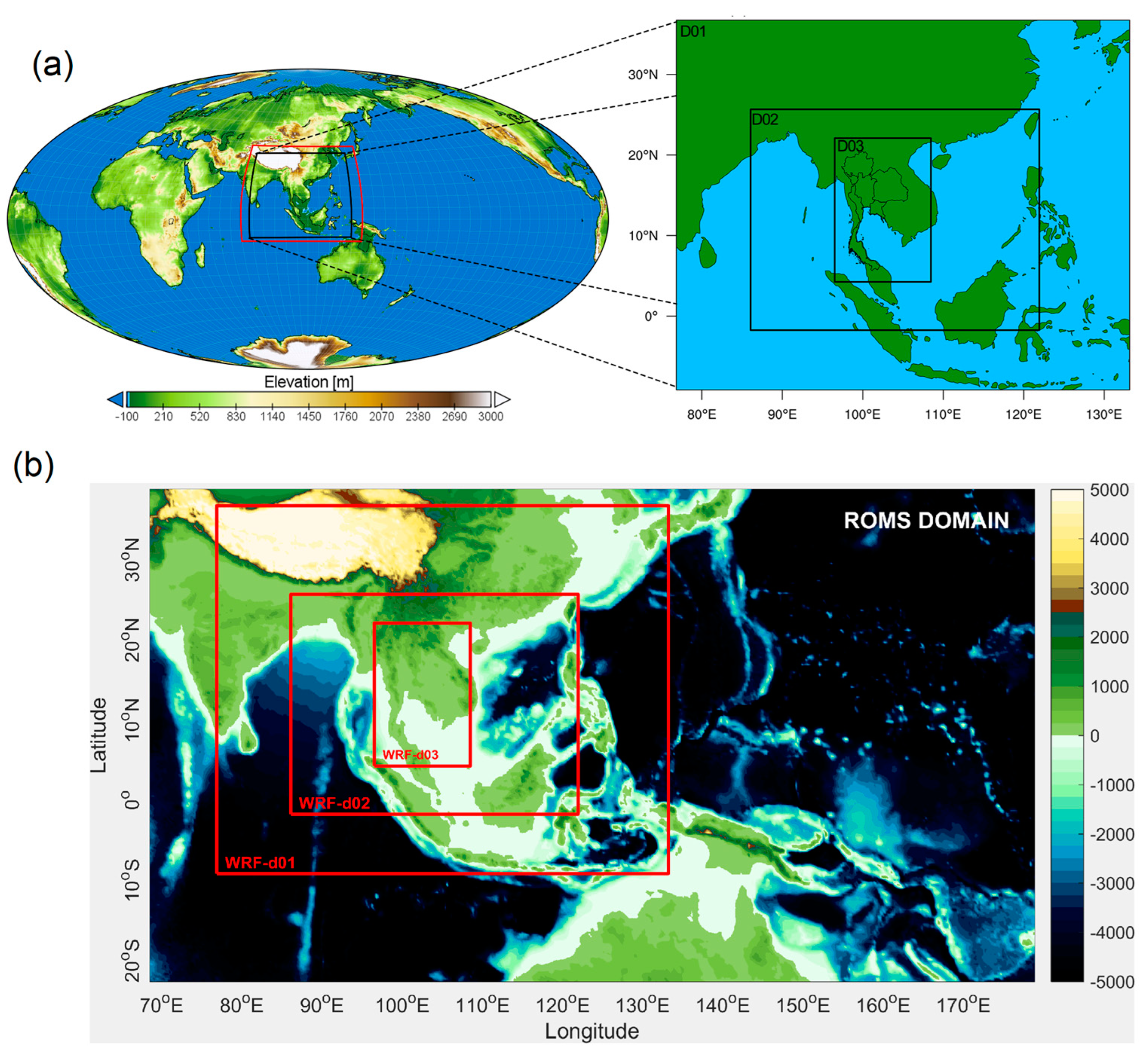
2.2.4. Modeling Domains

In this study, we employed the COAWST version 3.2, specifically activating the coupling between the WRF model and ROMS, to simulate a target selection of seven rainfall events (refer to Table 1). Our configuration of the WRF model consisted of three nested domains with respective resolutions of 27 km (D01), 9 km (D02), and 3 km (D03), accompanied by 33 vertical levels. The outermost domain encompassed a significant area of Greater East Asia, encompassing South Asia, Southeast Asia, and East Asia, while the finest domain covered the entirety of Thailand, as Figure 3a illustrates. The ROMS domain with a horizontal resolution of 25 km2 and with 15 vertical layers spanned from 70 °E to 180 °E and 20 °S to 35 °N, ensuring comprehensive coverage of the influences of SST on atmospheric processes in the BoB and the SCS (Figure 3b).
In each of the target date simulations, the WRF model was initialized and driven with three different model lead times as defined in Table 1. Meteorological information being used for initialization and driving forces of the WRF model was obtained from the 6-hour Global Forecast System (GFS), developed by the National Centers for Environmental Prediction (NCEP) and freely available online at https://www.emc.ncep.noaa.gov/emc/pages/numerical_forecast_systems/gfs.php (accessed on 15 October 2023) [67]. Initial conditions for the ROMS model, fields of currents, salinity, and temperature are obtained from the global HYCOM simulation via https://www.hycom.org/dataserver/gofs-3pt1/analysis (accessed on 15 October 2023) [68]. In this configuration, the ROMS model exchanges SST with WRF every 3600 s (1 h). Then, the atmospheric model utilizes the received SST information as a boundary condition and reciprocally sends turbulent heat fluxes to the oceanic model [38]. By adopting this approach, ROMS can provide high-resolution and dynamically consistent SST updates. Moreover, the heat fluxes transmitted from WRF to ROMS are based on the SST received from ROMS, ensuring a coherent treatment of energy and momentum exchange [69].

2.3. Statistical Evaluation Metrics

For statistical metrics, we employed the probability of detection (POD), false alarm (FAR), and critical success index (CSI), known as the treat score (TS) for model evaluation. The equations for these metrics are presented below:
POD   =   Hits Hits   +   Misses   ,
FAR   =   False   Alarms False   Alarms   +   Hits   ,   and
CSI   =   Hits Hits   +   Misses   +   False   Alarms
where:
  • Hits refer to the number of correctly detected events.
  • Misses refer to the number of events that were present but went undetected.
  • False Alarms refer to the number of incorrect detections or false positives.
The POD is a crucial metric for numerical weather prediction (NWP) by which it can provide an objective measure of the model’s ability to accurately predict the occurrence of specific weather phenomena or events. The FAR quantifies the ratio of false alarms to the total number of events predicted by the model. False alarms occur when the model predicts an event (such as rain, a storm, or a specific condition) that ultimately does not materialize. On the other hand, the CSI offers a comprehensive assessment of a model’s support for decision-making by simultaneously evaluating its success in correctly predicting events and accounting for prediction errors. Hence, the metrics are particularly important for high-impact weather events, such as severe storms or heavy rainfall, which can have significant societal and economic consequences, making their accurate prediction of utmost importance. Evaluating the evaluation metrics allows forecasters and researchers to assess the model’s performance in capturing and predicting such high-impact events, which aids in decision-making and risk mitigation. In our explanation, we will express the statistical values as a percentage.
To provide a comprehensive evaluation of the model’s performance, by considering POD along with other metrics, forecasters and researchers can assess not only the model’s detection capability but also its ability to minimize false alarms and capture the overall forecast skill. Furthermore, in order to gain a more comprehensive understanding of the model’s prediction skill, the analysis is divided into six distinct regions of Thailand (see Figure 3) considering the regional average of the evaluation metrics.
Note that, for model evaluation, a systematic approach is employed. Firstly, observed and simulated rain intensity data, specifically for heavy and violent categories, are extracted for each target date. The simulated values are then compared against the corresponding observed values for the seven selected events. Consequently, the statistical values presented here represent an overall assessment of the model’s performance across all events rather than a specific case. To maintain consistency, the observed rainfall data are interpolated to match the highest horizontal resolution of the model used in the analysis (3 × 3 km2). This ensures that both observed and simulated datasets undergo identical analysis procedures, facilitating an objective and unbiased evaluation.

3. Results

3.1. Probability of Detection (POD) of Rainfall Forecast over Thailand during the Selected Events

Figure 4 shows the POD for rainfall forecasts in Thailand during the selected events. We categorized the forecasts into four distinct rainfall categories, as defined by the daily TMD criteria and compared them with the observation with a primary focus on the accurate prediction of heavy and violent rainfall events.
In the case of light rain, employing a specific set of BMJ combinations exhibits a higher POD across all lead-time forecasts, as Figure 4a–c depicts. It is noteworthy that the BMJ combination, particularly with the more complex MP schemes such as LIN and WSM3, exhibits a slightly superior POD performance ranging from 10.0 to 20.0% compared to CTRL, depending on the lead time. On the other hand, the POD values for other combinations remain comparable to CTRL for the initial lead-time forecast, with a slight decrease of 5–10% as the lead-time forecast increases. In the case of moderate rainfall, the CTRL and a specific set of G3 combinations demonstrate superior performance, accurately forecasting the POD at around 45–50%. Conversely, lower skill is observed in other combinations, particularly in a set of KF combinations.
When it comes to predicting heavy to violent rainfall, the model outperforms the control run (CTRL, depicted by the red dashed line), particularly in terms of POD. Specifically, the model attains significantly improved accuracy rates of 10% for heavy rainfall events and an impressive 50% for violent rainfall events when utilizing a combination of KF + ETA for heavy rainfall and KF + LIN for violent rainfall. Remarkably, the model employing the KF combinations with ETA, LIN, and WSM3 consistently demonstrates similar performance but consistently outperforms the other combinations in all lead-time predictions. When considering forecasts for violent rainfall, as Figure 4 shows, it is seen that the combination of BMJ, G3, and KF, coupled with LIN microphysics, consistently outperforms other combinations. This combination, particularly when paired with KF, yields the highest POD at approximately 80% for lead-0. For subsequent lead times, the set of KF combinations consistently exhibits high prediction skill (POD > 60%), while lower predictions (POD < 30%) are observed in the other combinations.

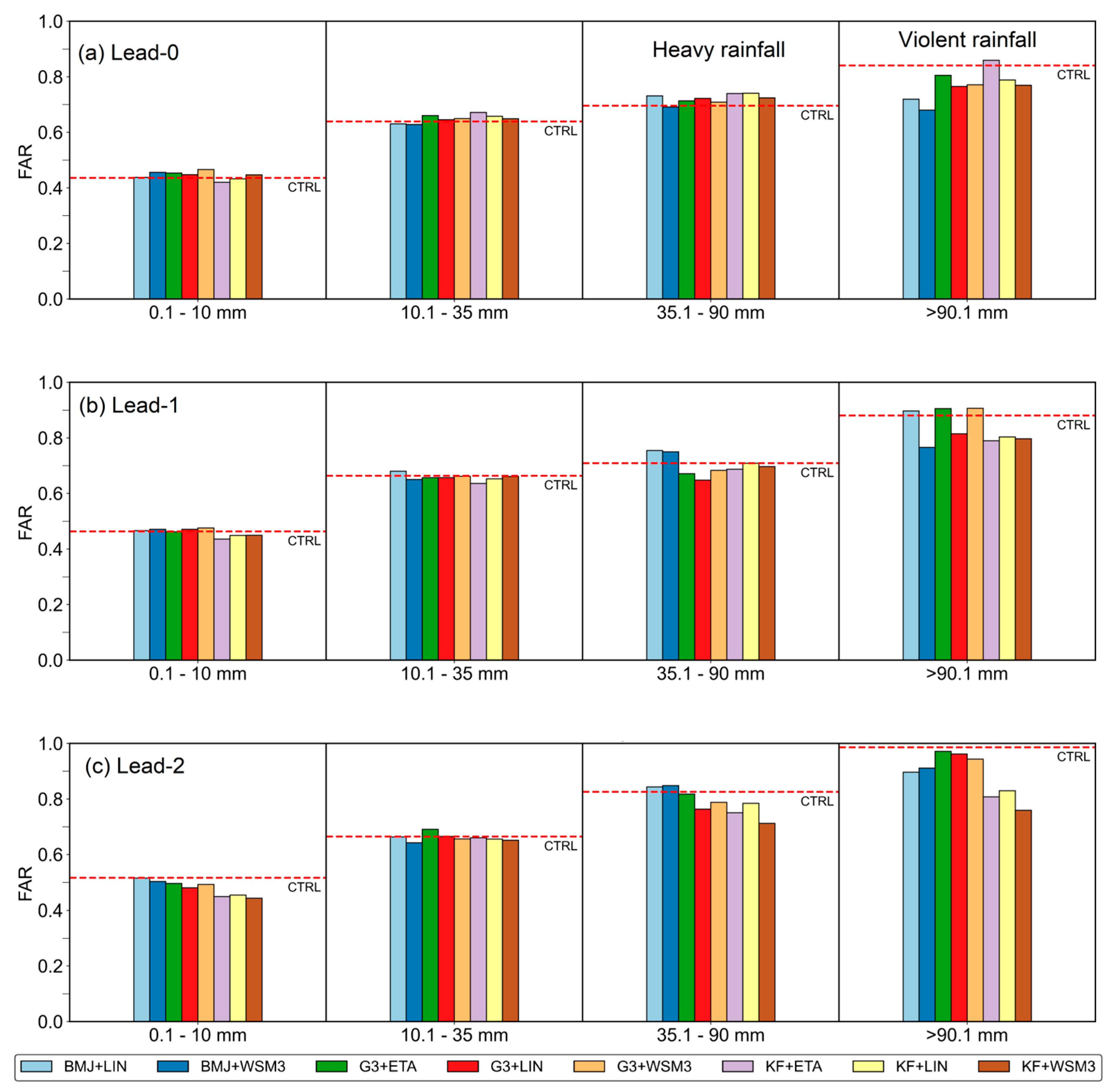
3.2. False Alarm Ratio (FAR) of Rainfall Forecast over Thailand during the Selected Events

To quantify the frequency of false alarms or inaccurate predictions of rainfall occurrence, we calculated the FAR for each rainfall category, as Figure 5 depicts. In general, the FAR values for the CTRL in predicting light to moderate rainfall are similar to those obtained from all combinations, with magnitudes ranging from 50% to 70%. Notably, both the CTRL and other combinations exhibit an increase in FAR as the lead-time forecast and rain intensity increase (Figure 5a–c). Regarding heavy rainfall, the FAR values for the CTRL and all combinations are comparable, with the highest FAR reaching 80% at a lead-time-2. Moreover, it is evident that the FAR is significantly higher in the BMJ combination set in capturing heavy rainfall compared to the others, while improved predictions of intense rainfall are observed in the KF scheme combinations, exhibiting lower FAR values, particularly for longer lead-time forecasts.

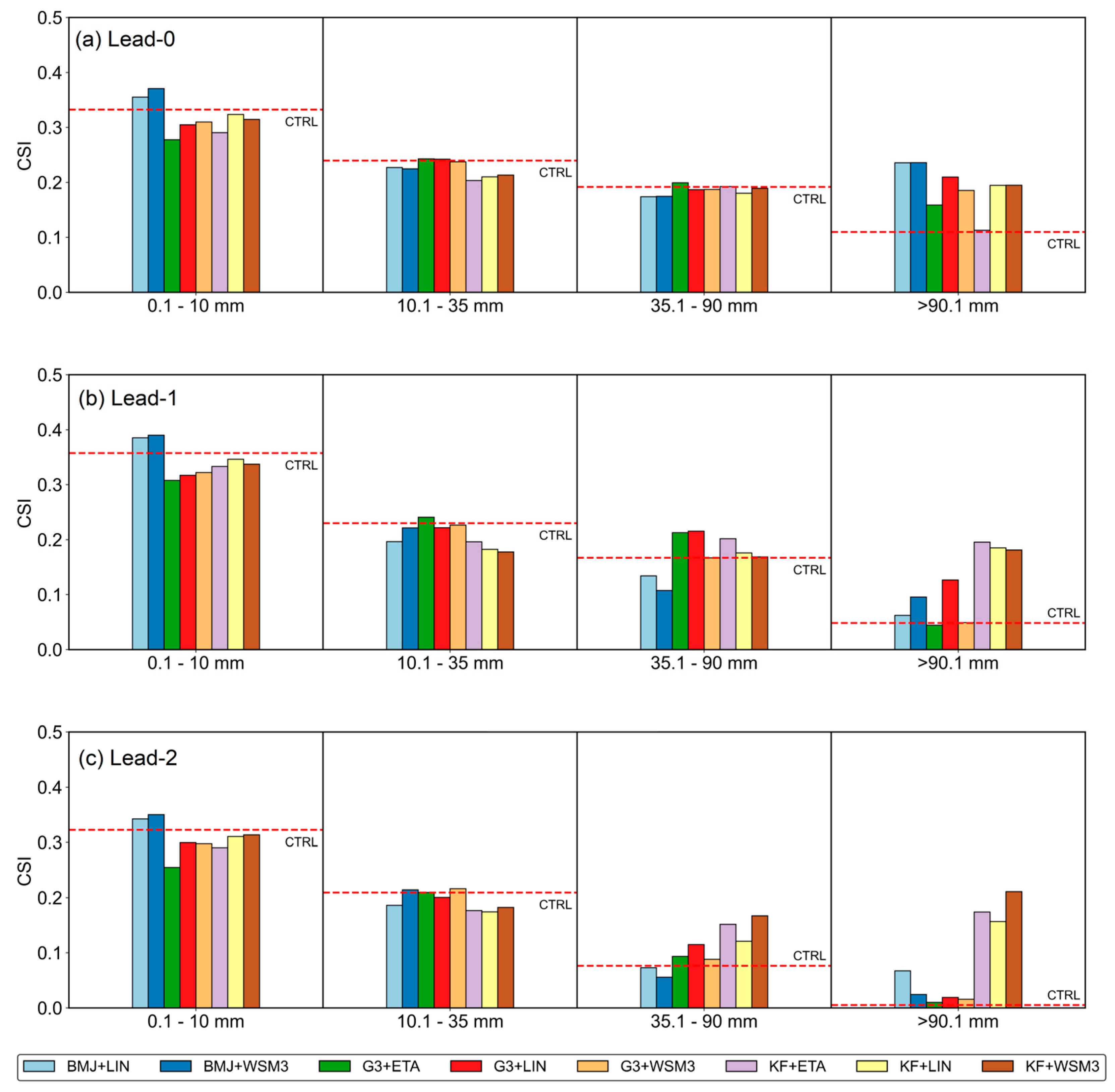
3.3. Critical Success Index (CSI) of Rainfall Forecast over Thailand during the Selected Events

The CSI was calculated to assess the performance of rainfall forecasts and given in Figure 6. Note that a higher CSI value indicates a more skillful and accurate forecast. As seen, CTRL and all combinations are comparable in prediction of light rain to heavy rain categories in all lead-time forecasts (Figure 6a–c). By analyzing the CSI values, it was observed that the CTRL run and all combinations exhibited comparable performance in predicting rainfall across the categories of light to heavy rain, regardless of lead-time forecasts (Figure 6a–c). The CSI values revealed varying levels of success for the rainfall forecasts during the selected events. Specifically, light rain events demonstrated higher CSI values, particularly in the set of BMJ combinations (35–40%), followed by the set of KF combinations (30–35%), indicating a stronger agreement between the forecasted and observed rainfall occurrences compared to other rainfall categories. However, it is worth noting that the prediction skill of the CTRL decreased as the intensity of rainfall increased, particularly for violent rainfall, which exhibited very low skill (CSI < 10%) at higher lead-time forecasts (Figure 6c). It was also noticed that the model consistently shows better prediction of heavy to violent rainfall in almost all lead-time forecasts when employing the KF scheme, specifically in lead-time-1 and lead-time-2. However, the prediction of the intense rainfall categories was still limited with CSI values less than 20%.

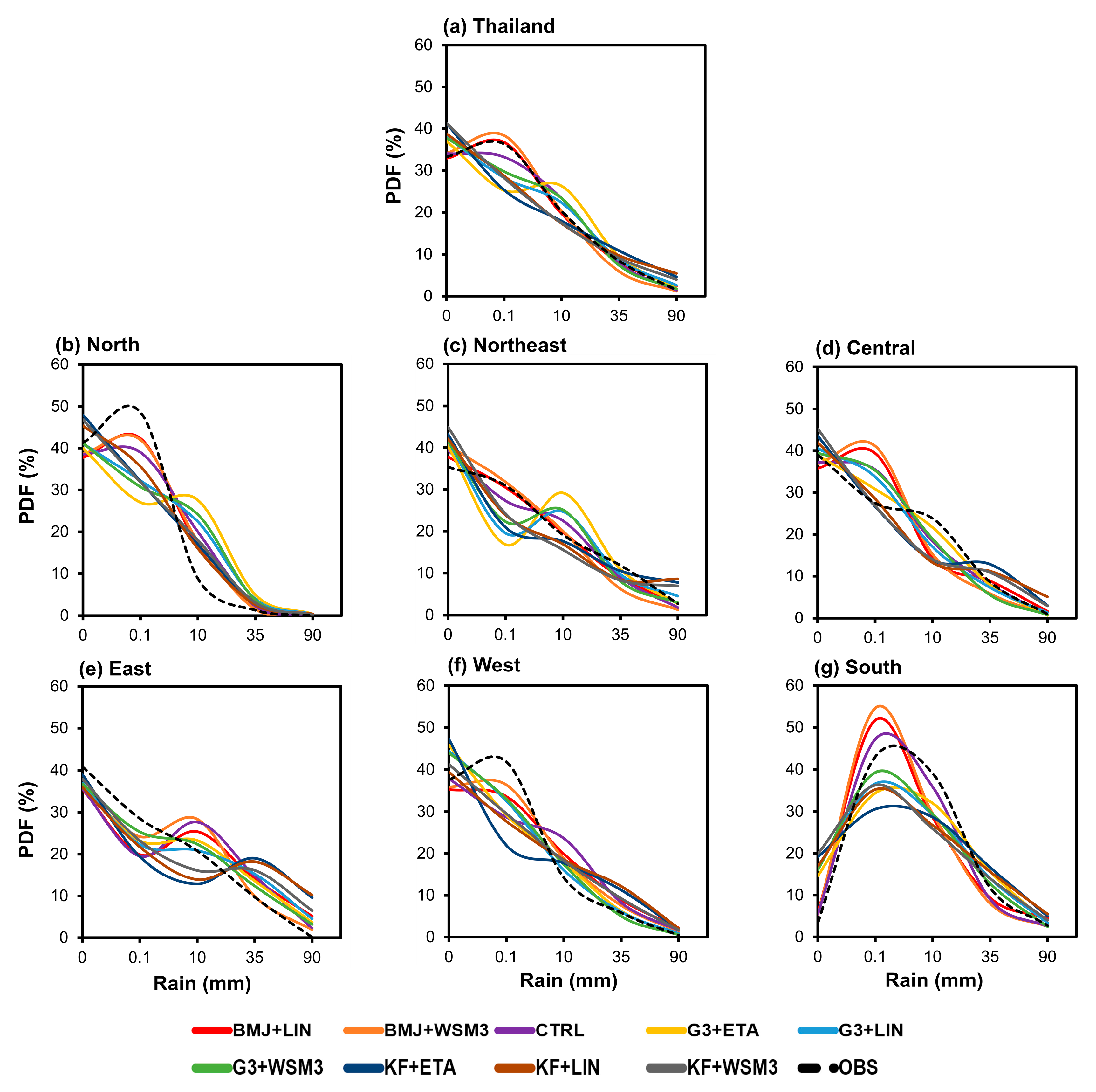
3.4. Probability Distribution Function (PDF) of Daily Rainfall over Thailand during the Selected Events

In addition to the previously mentioned validation, there exists a supplementary interest in expanding our evaluation to encompass the probability distribution function (PDF) of daily rainfall during the selected extreme events across Thailand. This endeavor is undertaken with the purpose of understanding the probability distribution of daily rainfall and conducting a comparative analysis against simulations given by the different CU and MP combinations, categorized according to the TMD’s daily rainfall classification (Figure 7).
Based on the selected rainfall events in 2020, the observed intensity distribution of daily rainfall over Thailand reveals a distinct asymmetry (Figure 7a). As seen, approximately 40% of rain events are associated with trace rain (<0.1 mm), while 20–30% are characterized by light rain (0.1–10.0 mm). Additionally, 10–15% of rainy days featured moderate rain (10.1–35.0 mm), and less than 10% are marked by heavy to violent rainfall. When we assess the agreement between the observed and simulated distributions, it becomes evident that the combined BMJ + LIN and BMJ + WSM3 display a noteworthy alignment with the observed PDF across all rainfall categories. In contrast, other combinations of cumulus and microphysics options tend to exhibit certain discrepancies, specifically overestimation (underestimation) for zero or nearly zero (trace to light) rainfall categories. For the moderate rain, it is worth noting that the observed PDF and the predictions are generally comparable, except for the G3 combinations, which overestimate the observed rainfall distribution for the category. Regarding heavy to violent rainfall, our results suggest that most of the combinations provide relatively accurate estimates for the long tail of extreme rainfall events. However, the BMJ + WSM3 (a set of KF combinations) slightly underestimate (overestimate) these events.
Furthermore, we conducted a comprehensive assessment of rainfall intensity distribution during the selected 2020 events across six distinct sub-regions of Thailand: north, northeast, central, east, west, and the south, as Figure 7b–g shows. Our analysis reveals variations in the density distribution of rainfall events, which vary across these regions, reflecting the distinct spatial impacts of tropical storms and atmospheric disturbances in each area. In the northern region, an examination of the PDF reveals a positively skewed gamma distribution. This distribution indicates that roughly 50% of recorded rainfall events can be attributed to trace rain, with less than 30% and 10% associated with light and moderate rain, respectively. The occurrence of heavy to violent rainfall events is exceptionally rare, accounting for less than 5% of the total (Figure 7b).
Indeed, the daily rainfall density functions in the northeast, central, and eastern regions closely align with negatively skewed linear tail-fitted curves (Figure 7c–e). These curves signify an asymmetrical distribution of rainfall intensities in these sub-regions, with a propensity for more frequent instances of lighter rainfall (35–40%) and progressively fewer occurrences of heavier rainfall. Approximately 20–30% of the recorded events fall within the moderate to violent rainfall categories. It is worth noting that this distribution pattern aligns with the observed heavy rainfall events in 2020, and typically occurred in these sub-regions (see Figure 2).
Regarding the western sub-region’s rainfall distribution, it is evident that it closely adheres to a gamma-fitted distribution with a positive skewness by which about 45% of rainfall events are attributed to trace rain, with 20–35% associated with light rain, 5–10% categorized as moderate, and less than 5% falling into the heavy to violent rainfall category (Figure 7f). Unlike the other sub-region, in the south, while it may not exhibit a perfect fit, its rainfall distribution closely approximates a normal curve (Figure 7g). Occurrences of zero and trace rain are infrequent, constituting less than 5%. The majority of rainfall events are concentrated within the light to moderate rain categories, ranging from 20 to 40%, with heavy to violent rainfall events making up less than 10%.
For prediction, our findings indicate that predicting the observed daily rainfall distribution can be a challenging task for the model. The skill of prediction depends on the specific geographical region and the combination of CU and MP. For instance, in the north, we observed that none of the combinations can effectively replicate the shape of the observed PDF of rainfall distribution. The model tends to exhibit tendencies of overestimation (underestimation) of the occurrence of trace (light) rain (Figure 7b). Similarly, in the northeastern sub-region where extreme rainfall events were particularly prevalent in 2020, the model cannot provide accurate estimations of the sub-regional rainfall distribution in most combinations. The exception is the BMJ + LIN combination, which closely aligns with observed data (Figure 7c). In addition, we observed that most combinations perform well in estimating the frequency of heavy to violent rainfall events in the northeast. However, a subset of KF combinations tends to slightly overestimate the tail end of rainfall distribution in the sub-region by approximately 5%.
In the central sub-region, a particular group of combinations involving BMJ and G3 tends to exhibit a substantial tendency to overestimate trace rain occurrences, whereas the KF combination consistently provides more accurate estimations for this rainfall category. Furthermore, the model tends to underestimate the occurrence of light to moderate rain across all combinations. However, the G3 + ETA combination stands out as the most reliable in terms of estimating this category accurately. For heavy to violent rainfall, combinations, that is, BMJ + LIN, G3 + ETA, and G3 + LIN outperform other combinations, closely aligning with the tail end of the observed PDF. Meanwhile, a set of KF combinations slightly overestimate (<5%) the long-tail of the observed distribution (Figure 7d).
In the eastern sub-region, the model exhibits poor accuracy in predicting the observed rainfall distribution across all combinations and rainfall categories (Figure 7e). Notably, within this sub-region, all combinations underestimate trace rain events while overestimating the occurrence of heavy to violent rainfall. Additionally, specific combinations involving BMJ and G3 exhibit an overestimation of the frequency of light to moderate rain, while a subset of KF combinations underestimates the occurrence of these rainfall events. In the western sub-region, the model underestimates the occurrences of trace to light rain events for all combinations. However, it does perform well in estimating non-rainfall events for most combinations, except for a set of G3 combinations and KF + ETA, which notably overestimates non-rainfall events by approximately 10% (Figure 7f). In the south, the shape of the observed rainfall distribution is well approximated by the model across all combinations. The model closely captures, although not perfectly fitting, the peak of the distribution, which corresponds to trace to light rain events. Notably, the CTRL combination (i.e., BMJ + ETA) outperforms other combinations in this sub-region.

4. Discussion

The results unveiled both commendable strengths and notable weaknesses in the models’ performance. The models excelled in accurately predicting light to moderate rainfall, and some model combinations exhibited a higher level of proficiency in specific rainfall categories. However, forecasting heavy and intense rainfall posed a more formidable challenge, resulting in limited success across various model combinations and lead-time forecasts. Wu et al. [18] also highlighted limitations in forecasting heavy to violent rainfall, particularly in response to tropical disturbances and storms. They suggested that this difficulty might be attributed to the intricate and nonlinear interactions among storm-related factors, which encompass dynamics, heat, cloud microphysics, and radiation.
Regarding the POD, the model performance varied across different rainfall categories and lead-time forecasts. In the case of light rain, specific combinations, particularly the BMJ combinations with LIN and WSM3 microphysical options, exhibited higher POD values compared to the CTRL. However, other combinations showed comparable performance to CTRL, except for a slight decrease in POD as the lead time increased. For moderate rainfall, CTRL and specific G3 combinations demonstrated superior performance with POD values around 45–50%. Conversely, the KF combinations showed lower skill in predicting moderate rainfall. For heavy rainfall, certain G3 and KF combinations, particularly when combined with ETA and LIN microphysical options, showed improved results compared to CTRL. In the case of violent rainfall, the combination of BMJ, G3, and KF, along with LIN microphysics, outperformed other combinations, especially when combined with KF for lead-0. The KF combinations consistently exhibited high prediction skill for subsequent lead times, while lower predictions were observed in other combinations.
In terms of the FAR, both CTRL and the combination models showed similar performance in predicting light to moderate rainfall. The FAR values increased as the lead-time forecast and rain intensity increased. For heavy rainfall, the FAR values were comparable between CTRL and the combination models, with the highest FAR observed at lead-time-2. The BMJ combinations showed higher FAR values in capturing heavy rainfall, while the KF scheme combinations exhibited improved predictions of intense rainfall with lower FAR values, particularly for longer lead-time forecasts.
The CSI analysis revealed that CTRL and the combination models exhibited comparable performance in predicting rainfall across light to heavy rain categories and various lead-time forecasts. Light rain events showed higher CSI values, particularly in the BMJ and KF combinations, indicating a stronger agreement between the forecasted and observed rainfall occurrences. However, the prediction skill of CTRL decreased as the intensity of rainfall increased, especially for violent rainfall, with very low CSI values at higher lead-time forecasts. It is worth noting that the KF scheme consistently showed better prediction of heavy to violent rainfall in almost all lead-time forecasts. However, the prediction of intense rainfall categories remained limited.
The study also offered valuable insights into the model’s ability to predict density distribution of daily rainfall across different geographical sub-regions of Thailand and combinations of CU and MP, revealing substantial variability in predictive accuracy contingent upon specific geographical regions and combinations. In the northern sub-region, the model faces challenges in accurately replicating the observed rainfall distribution’s shape, particularly in trace and light rain categories, resulting in instances of both overestimation and underestimation. In the northeastern sub-region, characterized by extreme rainfall events in 2020, the model has difficulty in providing precise estimations across most combinations, with an exception found in the BMJ + LIN combination.
The central sub-region exhibits unique challenges, with BMJ and G3 combinations tending to overestimate trace rain, and the KF combination offering more accurate estimates. Notably, the G3 + ETA combination excels in estimating light to moderate rain. For heavy to violent rainfall, combinations such as BMJ + LIN, G3 + ETA, and G3 + LIN perform well, albeit with slight overestimations by KF combinations.
The eastern sub-region presents considerable difficulty, with consistent underestimations of the probability distribution of trace rain and overestimations of heavy to violent rainfall, along with overestimations of the density of light to moderate rain by BMJ and G3 combinations and underestimations by KF combinations.
The western sub-region is characterized by underestimations of the occurrence of trace to light rain events across all combinations, while non-rainfall (zero rain intensity) events are well estimated in most cases, except for G3 combinations and KF + ETA, which notably overestimate non-rainfall events.
In the south, the model closely approximates the observed rainfall distribution, particularly the peak corresponding to trace to light rain events, with the BMJ + ETA (CTRL) combination performing most effectively in this sub-region. It is worth noting that while our suggested combination proves optimal for this sub-region, it may not align with the findings of Kirtsaeng et al. [70], who advocated for KF as a preferable option over BMJ and G3 for the southern sub-regions. This disparity between our study and the previous one could stem from differences in the analyzed rainfall events. The prior research focused on a single instance of heavy rainfall, heavily influenced by a monsoon system rather than the dynamics of a tropical storm or atmospheric distribution. Additionally, the earlier study employed their simulation based on a microphysics option.
These findings emphasize the region-specific complexities and underscore the necessity of tailored approaches for enhancing rainfall predictions, particularly in regions with unique characteristics or extreme weather events.

5. Conclusions

This study addresses the persistent challenge of accurately predicting heavy to violent rainfall events in Thailand, often associated with tropical storms and atmospheric disturbances. The innovative approach employed here, utilizing the coupled WRF-ROMS, aimed to optimize MP and CU parameterization schemes. Three CU schemes (i.e., BMJ, G3, KF) and three MP schemes (i.e., ETA, LIN, WSM3) were rigorously evaluated in seven instances of heavy to violent rainfall events during June to December of 2020. The performance assessment using POD, FAR, and CSI metrics revealed that while the models showed proficiency in predicting light to moderate rainfall, forecasting heavy and violent rainfall remained challenging, especially for longer lead-time forecasts. Based on the evaluation metrics, the study reveals several key findings. Notably, certain combinations, including BMJ and KF with LIN microphysics, demonstrate improved POD performance, particularly in predicting heavy and violent rainfall events. However, challenges persist, such as higher FAR values for intense rainfall predictions, especially in a set of the BMJ combinations. The CSI values reflect the varying success rates across rainfall categories, with light rain events showing higher skill.
According to the analysis of probability distribution of daily rainfall, it is evident that certain combinations of CU and MP parameterizations exhibit superior performance in predicting the rainfall distributions over Thailand and its sub-regions. Notably, the BMJ + LIN combination stands out as an effective choice in accurately estimating rainfall distribution overall in Thailand, especially in the northern sub-region. In the northeastern sub-region, where extreme rainfall events were prevalent in 2020, the BMJ + LIN combination also aligns well with observed density distribution. Additionally, the G3 + ETA combination demonstrates strong predictive capabilities, especially in estimating density of light to moderate rain in the central sub-region. In the South, the CTRL combination (BMJ + ETA) emerges as the most effective choice for approximating the observed rainfall distribution.
In summary, these findings emphasize the critical importance of carefully selecting cumulus and microphysics parameterizations that are tailored to the specific geographical characteristics and rainfall patterns when conducting predictive modeling for Thailand. These customized approaches have the potential to significantly enhance the accuracy of rainfall forecasts, thereby offering valuable insights for decision-making processes related to water resource management, flood control, and disaster preparedness in the region. Furthermore, our study sheds light on the unique challenges and strengths of the model in predicting the density distribution of daily rainfall. It underscores the necessity of exploring various combinations of cumulus and microphysics parameterizations, particularly in the context of tropical storms and atmospheric disturbances. While the results presented here are derived from the analysis of seven selected significant rainfall events modulated by tropical storms and atmospheric disturbances in 2020, it is essential to establish statistical significance through a more extensive sampling of case studies. This expanded dataset should also account for major atmospheric factors, such as the Madden–Julian Oscillation (MJO), known to exert a profound influence on rainfall patterns in Thailand. Additionally, it is worth mentioning that previous studies, such as Efstathiou et al. [30] and references therein, have indicated that the choice of boundary layer schemes had a limited impact on the simulation of heavy rainfall. While this aspect was not specifically addressed in the present study, it remains a subject for further investigation and consideration in future research efforts.

Author Contributions

Conceptualization and methodology, K.T.; validation, K.T., A.F., P.P. and J.A.; formal analysis, R.S. and J.A.; investigation, K.T.; data curation, A.F., P.P. and R.S.; writing—original draft preparation, K.T. and A.F.; visualization, A.F., P.P. and R.S.; funding acquisition, K.T.; writing—review and editing, K.T. and K.S. All authors have read and agreed to the published version of the manuscript.

Funding

This research was funded by the Science, Research and Innovation Promotion Fund (SRI), Thailand Science Research and Innovation (TSRI), grant number 48873, 160399, and 180529 under the Sub-Seasonal to Seasonal (S2S) Prediction Project for Disaster Risk Reduction and Water Management in Thailand (S2S Thailand Project).

Institutional Review Board Statement

Not applicable.

Informed Consent Statement

Not applicable.

Data Availability Statement

Readers can find data availability of the WRF-ROMS forecast and NHC via https://www.thaiwater.net/. For details of the meteorological data over Thailand, they are available upon request by contacting K.T.

Acknowledgments

The authors sincerely thank the NHC for the daily rainfall station data and the USGS for availability of the COAWST modeling system. We also acknowledge the National Science and Technology Development Agency (NSTDA) Supercomputer Center (ThaiSC) for providing computing resources for this work. The authors would like to extend their sincere gratitude to all the reviewers for their valuable insights and constructive feedback, which have significantly contributed to the enhancement of this work.

Conflicts of Interest

The authors declare no conflict of interest.

References

  1. Gray, W.M. Global view of the origin of tropical disturbances and storms. Mon. Weather Rev. 1968, 96, 669–700. [Google Scholar] [CrossRef]
  2. Bruyère, C.L.; Holland, G.J.; Towler, E. Investigating the Use of a Genesis Potential Index for Tropical Cyclones in the North Atlantic Basin. J. Clim. 2012, 25, 8611–8626. [Google Scholar] [CrossRef]
  3. Byers, H. Atmospheric Turbulence and the Wind Structure Near the Surface of the Earthin General Meteorology; McGraw-Hill Book Company Inc.: New York, NY, USA, 1944; Chapter XXIV. [Google Scholar]
  4. Emanuel, K.A. An Air-Sea Interaction Theory for Tropical Cyclones. Part I: Steady-State Maintenance. J. Atmos. Sci. 1986, 43, 585–605. [Google Scholar] [CrossRef]
  5. Krishnamurti, T.N.; Molinari, J.; Pan, H.-l.; Wong, V. Downstream Amplification and Formation of Monsoon Disturbances. Mon. Weather Rev. 1977, 105, 1281–1297. [Google Scholar] [CrossRef]
  6. Saha, K.; Sanders, F.; Shukla, J. Westward Propagating Predecessors of Monsoon Depressions. Mon. Weather Rev. 1981, 109, 330–343. [Google Scholar] [CrossRef]
  7. Chen, T.-C.; Chen, J.-M. The 10–20-Day Mode of the 1979 Indian Monsoon: Its Relation with the Time Variation of Monsoon Rainfall. Mon. Weather Rev. 1993, 121, 2465–2482. [Google Scholar] [CrossRef]
  8. Takahashi, H.G.; Yasunari, T. Decreasing Trend in Rainfall over Indochina during the Late Summer Monsoon: Impact of Tropical Cyclones. J. Meteorol. Soc. Jpn. Ser. II 2008, 86, 429–438. [Google Scholar] [CrossRef]
  9. Takahashi, H.G.; Fujinami, H.; Yasunari, T.; Matsumoto, J.; Baimoung, S. Role of Tropical Cyclones along the Monsoon Trough in the 2011 Thai Flood and Interannual Variability. J. Clim. 2015, 28, 1465–1476. [Google Scholar] [CrossRef]
  10. Li, H.; Hu, A.; Meehl, G.A. Role of Tropical Cyclones in Determining ENSO Characteristics. Geophys. Res. Lett. 2023, 50, e2022GL101814. [Google Scholar] [CrossRef]
  11. Shariful, F.; Sedrati, M.; Ariffin, E.H.; Shubri, S.M.; Akhir, M.F. Impact of 2019 Tropical Storm (Pabuk) on Beach Morphology, Terengganu Coast (Malaysia). J. Coast. Res. 2020, 95, 346–350. [Google Scholar] [CrossRef]
  12. Gale Emma, L.; Saunders Mark, A. The 2011 Thailand flood: Climate causes and return periods. Weather 2013, 68, 233–237. [Google Scholar] [CrossRef]
  13. Lim Han, S.; Boochabun, K. Flood generation during the SW monsoon season in northern Thailand. Geol. Soc. Lond. Spec. Publ. 2012, 361, 7–20. [Google Scholar] [CrossRef]
  14. Benfield, A. 2011 Thailand Floods Event Recap Report: Report of Impact Forecasting-March 2012; Impact Forecasting LLC, Aon Benfield Corporation: Chicago, IL, USA, 2012; pp. 7–10. [Google Scholar]
  15. Hydro-Informatics Institute. Record Water Events. Available online: https://www.thaiwater.net/report#flood (accessed on 16 May 2023).
  16. Islam, T.; Srivastava, P.K.; Rico-Ramirez, M.A.; Dai, Q.; Gupta, M.; Singh, S.K. Tracking a tropical cyclone through WRF–ARW simulation and sensitivity of model physics. Nat. Hazards 2015, 76, 1473–1495. [Google Scholar] [CrossRef]
  17. Potty, J.; Oo, S.M.; Raju, P.V.S.; Mohanty, U.C. Performance of nested WRF model in typhoon simulations over West Pacific and South China Sea. Nat. Hazards 2012, 63, 1451–1470. [Google Scholar] [CrossRef]
  18. Wu, Z.; Alshdaifat, N.M. Simulation of Marine Weather during an Extreme Rainfall Event: A Case Study of a Tropical Cyclone. Hydrology 2019, 6, 42. [Google Scholar] [CrossRef]
  19. Sivaprasad, P.; Samah, A.A.; Babu, C.A.; Fang, Y.; Mohd Nor, M.F.F.; Chenoli, S.N.; Cheah, W.; Mazuki, M.Y.A. Simulation of the atmospheric parameters during passage of a tropical storm over the South China Sea: A comparison with MetOcean buoy and ERA-Interim data. Meteorol. Appl. 2020, 27, e1895. [Google Scholar] [CrossRef]
  20. Benedetti, A.; Reid, J.S.; Knippertz, P.; Marsham, J.H.; Di Giuseppe, F.; Rémy, S.; Basart, S.; Boucher, O.; Brooks, I.M.; Menut, L.; et al. Status and future of numerical atmospheric aerosol prediction with a focus on data requirements. Atmos. Chem. Phys. 2018, 18, 10615–10643. [Google Scholar] [CrossRef]
  21. Doblas-Reyes, F.J.; García-Serrano, J.; Lienert, F.; Biescas, A.P.; Rodrigues, L.R.L. Seasonal climate predictability and forecasting: Status and prospects. WIREs Clim. Change 2013, 4, 245–268. [Google Scholar] [CrossRef]
  22. Monteiro, M.J.; Couto, F.T.; Bernardino, M.; Cardoso, R.M.; Carvalho, D.; Martins, J.P.A.; Santos, J.A.; Argain, J.L.; Salgado, R. A Review on the Current Status of Numerical Weather Prediction in Portugal 2021: Surface-Atmosphere Interactions. Atmosphere 2022, 13, 1356. [Google Scholar] [CrossRef]
  23. Linardakis, L.; Stemmler, I.; Hanke, M.; Ramme, L.; Chegini, F.; Ilyina, T.E.; Korn, P. Improving scalability of Earth system models through coarse-grained component concurrency—A case study with the ICON v2.6.5 modelling system. Geosci. Model Dev. 2022, 15, 9157–9176. [Google Scholar] [CrossRef]
  24. Baklanov, A.; Baldasano, J.M.; Bouchet, V.; Brunner, D.; Yang, Z. Coupled Chemistry-Meteorology/Climate Modelling (CCMM): Status and Relevance for Numerical Weather Prediction, Atmospheric Pollution and Climate Research Final GAW 226 10 May; WMO GAW Report; WMO: Geneva, Switzerland, 2016. [Google Scholar]
  25. Yesubabu, V.; Kattamanchi, V.K.; Vissa, N.K.; Dasari, H.P.; Sarangam, V.B.R. Impact of ocean mixed-layer depth initialization on the simulation of tropical cyclones over the Bay of Bengal using the WRF-ARW model. Meteorol. Appl. 2020, 27, e1862. [Google Scholar] [CrossRef]
  26. Srinivas, C.V.; Mohan, G.M.; Naidu, C.V.; Baskaran, R.; Venkatraman, B. Impact of air-sea coupling on the simulation of tropical cyclones in the North Indian Ocean using a simple 3-D ocean model coupled to ARW. J. Geophys. Res. Atmos. 2016, 121, 9400–9421. [Google Scholar] [CrossRef]
  27. Rajeswari, J.R.; Srinivas, C.V.; Mohan, P.R.; Venkatraman, B. Impact of Boundary Layer Physics on Tropical Cyclone Simulations in the Bay of Bengal Using the WRF Model. Pure Appl. Geophys. 2020, 177, 5523–5550. [Google Scholar] [CrossRef]
  28. Koh, T.-Y.; Fonseca, R. Subgrid-scale cloud–radiation feedback for the Betts–Miller–Janjić convection scheme. Q. J. R. Meteorol. Soc. 2016, 142, 989–1006. [Google Scholar] [CrossRef]
  29. Zhang, C.; Wang, Y. Why is the simulated climatology of tropical cyclones so sensitive to the choice of cumulus parameterization scheme in the WRF model? Clim. Dyn. 2018, 51, 3613–3633. [Google Scholar] [CrossRef]
  30. Efstathiou, G.A.; Zoumakis, N.M.; Melas, D.; Lolis, C.J.; Kassomenos, P. Sensitivity of WRF to boundary layer parameterizations in simulating a heavy rainfall event using different microphysical schemes. Effect on large-scale processes. Atmos. Res. 2013, 132–133, 125–143. [Google Scholar] [CrossRef]
  31. Hong, S.-Y.; Sunny Lim, K.-S.; Kim, J.-H.; Jade Lim, J.-O.; Dudhia, J. Sensitivity Study of Cloud-Resolving Convective Simulations with WRF Using Two Bulk Microphysical Parameterizations: Ice-Phase Microphysics versus Sedimentation Effects. J. Appl. Meteorol. Climatol. 2009, 48, 61–76. [Google Scholar] [CrossRef]
  32. Podeti, S.R.; Ramakrishna, S.S.V.S.; Viswanadhapalli, Y.; Dasari, H.; Nellipudi, N.R.; Rao, B.R.S. Sensitivity of Cloud Microphysics on the Simulation of a Monsoon Depression Over the Bay of Bengal. Pure Appl. Geophys. 2020, 177, 5487–5505. [Google Scholar] [CrossRef]
  33. Mohan, P.R.; Srinivas, C.V.; Yesubabu, V.; Baskaran, R.; Venkatraman, B. Tropical cyclone simulations over Bay of Bengal with ARW model: Sensitivity to cloud microphysics schemes. Atmos. Res. 2019, 230, 104651. [Google Scholar] [CrossRef]
  34. Sun, Y.; Zhong, Z.; Lu, W. Sensitivity of Tropical Cyclone Feedback on the Intensity of the Western Pacific Subtropical High to Microphysics Schemes. J. Atmos. Sci. 2015, 72, 1346–1368. [Google Scholar] [CrossRef]
  35. Maw, K.W.; Min, J. Impacts of Microphysics Schemes and Topography on the Prediction of the Heavy Rainfall in Western Myanmar Associated with Tropical Cyclone ROANU (2016). Adv. Meteorol. 2017, 2017, 3252503. [Google Scholar] [CrossRef]
  36. Lok, C.C.F.; Chan, J.C.L.; Toumi, R. Importance of Air-Sea Coupling in Simulating Tropical Cyclone Intensity at Landfall. Adv. Atmos. Sci. 2022, 39, 1777–1786. [Google Scholar] [CrossRef]
  37. Warner, J.C.; Armstrong, B.; He, R.; Zambon, J.B. Development of a Coupled Ocean–Atmosphere–Wave–Sediment Transport (COAWST) Modeling System. Ocean Model. 2010, 35, 230–244. [Google Scholar] [CrossRef]
  38. Warner, J.C.; Sherwood, C.R.; Signell, R.P.; Harris, C.K.; Arango, H.G. Development of a three-dimensional, regional, coupled wave, current, and sediment-transport model. Comput. Geosci. 2008, 34, 1284–1306. [Google Scholar] [CrossRef]
  39. Shchepetkin, A.F.; McWilliams, J.C. The regional oceanic modeling system (ROMS): A split-explicit, free-surface, topography-following-coordinate oceanic model. Ocean Model. 2005, 9, 347–404. [Google Scholar] [CrossRef]
  40. Haidvogel, D.B.; Arango, H.G.; Budgell, W.P.; Cornuelle, B.D.; Curchitser, E.N.; Lorenzo, E.D.; Fennel, K.; Geyer, W.R.; Hermann, A.J.; Lanerolle, L.; et al. Ocean forecasting in terrain-following coordinates: Formulation and skill assessment of the Regional Ocean Modeling System. J. Comput. Phys. 2008, 227, 3595–3624. [Google Scholar] [CrossRef]
  41. Skamarock, C.; Klemp, B.; Dudhia, J.; Gill, O.; Barker, D.M.; Duda, G.; Huang, X.; Wang, W.; Powers, G. A Description of the Advanced Research WRF Version 3. NCAR Tech. Note 2008, 475, 113. [Google Scholar]
  42. Spero, T.L.; Nolte, C.G.; Bowden, J.H.; Mallard, M.S.; Herwehe, J.A. The Impact of Incongruous Lake Temperatures on Regional Climate Extremes Downscaled from the CMIP5 Archive Using the WRF Model. J. Clim. 2016, 29, 839–853. [Google Scholar] [CrossRef]
  43. Zhang, Z.; Colle, B.A. Impact of Dynamically Downscaling Two CMIP5 Models on the Historical and Future Changes in Winter Extratropical Cyclones along the East Coast of North America. J. Clim. 2018, 31, 8499–8525. [Google Scholar] [CrossRef]
  44. Umer, Y.; Jetten, V.G.; Ettema, J.; Lombardo, L. Application of the WRF model rainfall product for the localized flood hazard modeling in a data-scarce environment. Nat. Hazards 2022, 111, 1813–1844. [Google Scholar] [CrossRef]
  45. D’Isidoro, M.; Briganti, G.; Vitali, L.; Righini, G.; Adani, M.; Guarnieri, G.; Moretti, L.; Raliselo, M.; Mahahabisa, M.; Ciancarella, L.; et al. Estimation of solar and wind energy resources over Lesotho and their complementarity by means of WRF yearly simulation at high resolution. Renew. Energy 2020, 158, 114–129. [Google Scholar] [CrossRef]
  46. Institute, H.-I. Weather Situation. Available online: https://www.thaiwater.net/weather/ (accessed on 24 May 2023).
  47. Hydro-Informatics Institute. Weather Situation: WRF-ROMS Rainfall Forecast. Available online: https://www.thaiwater.net/weather/rainfall (accessed on 11 May 2023).
  48. Torsri, K.; Wannawong, W.; Sarinnapakorn, K.; Boonya-Aroonnet, S.; Chitdon, R. An application of air-sea model components in the Coupled Ocean-Atmosphere-Wave-Sediment Transport (COAWST) Modeling System over an Indochina Peninsular sub-region: Impact of high spatiotemporal SST on WRF model in precipitation prediction. In Proceedings of the 2014 Asia Oceania Geosciences Society (2014 AOGS), Sapporo, Japan, 28 July–1 August 2014. [Google Scholar]
  49. Thai Meteorological Department (TMD). Daily Rainfall. Available online: http://www.arcims.tmd.go.th/dailydata/DetailDailyRain.html (accessed on 29 May 2023).
  50. TMD. The Tropical Cyclone That Occurred in the Covered Area in the Year 2020 (in Thai). Available online: http://climate.tmd.go.th/content/file/1917 (accessed on 7 July 2023).
  51. Baki, H.; Chinta, S.; Balaji, C.; Srinivasan, B. A sensitivity study of WRF model microphysics and cumulus parameterization schemes for the simulation of tropical cyclones using GPM radar data. J. Earth Syst. Sci. 2021, 130, 1–30. [Google Scholar] [CrossRef]
  52. Guo, Z.; Fang, J.; Sun, X.; Yang, Y.; Tang, J. Sensitivity of Summer Precipitation Simulation to Microphysics Parameterization Over Eastern China: Convection-Permitting Regional Climate Simulation. J. Geophys. Res. Atmos. 2019, 124, 9183–9204. [Google Scholar] [CrossRef]
  53. Janjic, Z.I. The Step-Mountain Eta Coordinate Model: Further Developments of the Convection, Viscous Sublayer, and Turbulence Closure Schemes. Mon. Weather Rev. 1994, 122, 927–945. [Google Scholar] [CrossRef]
  54. Zhao, Q.; Carr, F.H. A Prognostic Cloud Scheme for Operational NWP Models. Mon. Weather Rev. 1997, 125, 1931–1953. [Google Scholar] [CrossRef]
  55. Chen, S.-H.; Sun, W.-Y. A One-dimensional Time Dependent Cloud Model. J. Meteorol. Soc. Jpn. 2002, 80, 99–118. [Google Scholar] [CrossRef]
  56. Hong, S.Y.; Dudhia, J.; Chen, S.H. A Revised Approach to Ice Microphysical Processes for the Bulk Parameterization of Clouds and Precipitation. Mon. Weather Rev. 2004, 132, 103–120. [Google Scholar] [CrossRef]
  57. Grell, G.A.; Dévényi, D. A generalized approach to parameterizing convection combining ensemble and data assimilation techniques. Geophys. Res. Lett. 2002, 29, 38-1–38-4. [Google Scholar] [CrossRef]
  58. Kain, J.S. The Kain–Fritsch Convective Parameterization: An Update. J. Appl. Meteorol. 2004, 43, 170–181. [Google Scholar] [CrossRef]
  59. Raju, P.V.S.; Potty, J.; Mohanty, U.C. Sensitivity of physical parameterizations on prediction of tropical cyclone Nargis over the Bay of Bengal using WRF model. Meteorol. Atmos. Phys. 2011, 113, 125–137. [Google Scholar] [CrossRef]
  60. Rodrigo, C.; Kim, S.; Jung, I.H. Sensitivity Study of WRF Numerical Modeling for Forecasting Heavy Rainfall in Sri Lanka. Atmosphere 2018, 9, 378. [Google Scholar] [CrossRef]
  61. Raktham, C.; Bruyère, C.; Kreasuwun, J.; Done, J.; Thongbai, C.; Promnopas, W. Simulation sensitivities of the major weather regimes of the Southeast Asia region. Clim. Dyn. 2015, 44, 1403–1417. [Google Scholar] [CrossRef]
  62. Chotamonsak, C.; Salathé, E.; Kreasuwan, J.; Chantara, S. Evaluation of Precipitation Simulations over Thailand using a WRF Regional Climate Model. Chiang Mai J. Sci. 2012, 39, 623–628. [Google Scholar]
  63. University Corporation for Atmospheric Research. WRF-ARW V4: User’s Guide. Available online: https://www2.mmm.ucar.edu/wrf/users/docs/user_guide_v4/v4.2/WRFUsersGuide_v42.pdf (accessed on 25 May 2023).
  64. Nasrollahi, N.; Aghakouchak, A.; Li, J.; Gao, X.; Hsu, K.-l.; Sorooshian, S. Assessing the Impacts of Different WRF Precipitation Physics in Hurricane Simulations. Weather Forecast. 2012, 27, 1003–1016. [Google Scholar] [CrossRef]
  65. Venkata Rao, G.; Venkata Reddy, K.; Sridhar, V. Sensitivity of Microphysical Schemes on the Simulation of Post-Monsoon Tropical Cyclones over the North Indian Ocean. Atmosphere 2020, 11, 1297. [Google Scholar] [CrossRef]
  66. Penny, A.B.; Harr, P.A.; Doyle, J.D. Sensitivity to the Representation of Microphysical Processes in Numerical Simulations during Tropical Storm Formation. Mon. Weather Rev. 2016, 144, 3611–3630. [Google Scholar] [CrossRef]
  67. National Oceanic and Atmospheric Administration. The Global Forecast System (GFS). Available online: https://www.emc.ncep.noaa.gov/emc/pages/numerical_forecast_systems/gfs.php (accessed on 10 July 2023).
  68. Consortium for Data Assimilative Modeling. GOFS 3.1: 41-Layer HYCOM + NCODA Global 1/12° Analysis. Available online: https://www.hycom.org/dataserver/gofs-3pt1/analysis (accessed on 10 July 2023).
  69. Ricchi, A.; Miglietta, M.M.; Barbariol, F.; Benetazzo, A.; Bergamasco, A.; Bonaldo, D.; Cassardo, C.; Falcieri, F.M.; Modugno, G.; Russo, A.; et al. Sensitivity of a Mediterranean Tropical-Like Cyclone to Different Model Configurations and Coupling Strategies. Atmosphere 2017, 8, 92. [Google Scholar] [CrossRef]
  70. Kirtsaeng, S.; Kreasuwun, J.; Chantara, S.; Kirtsaeng, S.; Sukthawee, P.; Masthawee, F. The Weather Research and Forecasting (WRF) Model Performance for a Simulation of the 5 November 2009 Heavy Rainfall over Southeast of Thailand. Chiang Mai J. Sci. 2011, 39, 511–523. [Google Scholar]
Figure 1. Spatial distribution of rain gauges from the National Hydroinformatics Data Center (NHC) stations being used in this study. The colored dot points represent stations in six sub-regions of Thailand (i.e., north, central, northeast, west, east, and south).
Atmosphere 14 01574 g001
Figure 2. Spatial distribution of 24 h accumulated rainfall on the target date along with its associated synoptic weather chart at 00UTC as summarized in Table 1.
Atmosphere 14 01574 g002
Figure 3. Modeling domains of this study: (a) 3-nested WRF domains with (b) a single ROMS domain.
Atmosphere 14 01574 g003
Figure 4. POD of rainfall forecast for (a) Lead-0, (b) Lead-1, and (c) Lead-2 with different MP and CU combinations (CTRL is denoted by a red dashed line, while the remaining combinations are depicted as bar charts).
Atmosphere 14 01574 g004
Figure 5. FAR of rainfall forecast for (a) Lead-0, (b) Lead-1, and (c) Lead-2 with different MP and CU combinations (CTRL is denoted by a red dashed line, while the remaining combinations are depicted as bar charts).
Atmosphere 14 01574 g005
Figure 6. CSI of rainfall forecast for (a) Lead-0, (b) Lead-1, and (c) Lead-2 with different MP and CU combinations (CTRL is denoted by a red dashed line, while the remaining combinations are depicted as bar charts).
Atmosphere 14 01574 g006
Figure 7. Probability density function (PDF) of observed daily rainfall (OBS) during the selected events with the fit of gamma distribution for (a) overall Thailand and (bg) its sub-regions together with those predicted by the model with different CU and MP combinations.
Atmosphere 14 01574 g007
Table 1. Selected heavy rainfall events in Thailand associated with atmospheric disturbed conditions in the 2020 and experimental designs for model integration with three different lead times (Lead-0, 1, and 2).
Event
No.
Heay Rainfall Event (Target Date) *During StormModel Initial Date at 00 UTC
Lead-0
(24 h)
Lead-1
(48 h)
Lead-2
(72 h)
Event 114 JuneTD Nuri14 June13 June12 June
Event 21 AugustTD Sinlaku1 August31 July30 July
Event 318 SeptemberTS Noul18 September17 September16 September
Event 416 OctoberTD16 October15 October14 October
Event 512 NovembersTS Vamco12 November11 November10 November
Event 626 NovemberTC Nivar26 November25 November24 November
Event 71 DecemberTD1 December30 November29 November
TD: Tropical depression, TS: Tropical storm, sTS: Severe tropical storm, and TC: Tropical cyclone. * The target date refers to the date when the storm approaches or is in close proximity to Thailand, resulting in significant rainfall.
Table 2. Selected heavy rainfall events in Thailand associated with tropical storms and three model initial date/time runs for model validation.
EXPCUReferenceMPReference
CTRL *BMJJanjic [53]ETAZhao and Carr [54]
EXP-01BMJLINChen and Sun [55]
EXP-02BMJWSM3Hong et al. [56]
EXP-03G3Grell and Dévényi [57]ETA
EXP-04G3LIN
EXP-05G3WSM3
EXP-06KFKain [58]ETA
EXP-07KFLIN
EXP-08KFWSM3
* CTRL: Control run experiment.
Table 3. Summary of CU and MP used in this study [63].
CU SchemeMoisture TendenciesMomentum TendenciesShallow
Convection
BMJ-NoYes
G3Qc, QiNoYes
KFQc, Qr, Qi, QsNoYes
MP SchemeMass Variables
ETAQc, Qr, Qs (Qt*)
LINQc, Qr, Qi, Qs, Qg
WSM3Qc, Qr
Qc: cloud, Qi: ice, Qr: mixing ratio for rain, Qs: snow, Qg: graupel; Qt*: total water mixing ratio tendency.
Disclaimer/Publisher’s Note: The statements, opinions and data contained in all publications are solely those of the individual author(s) and contributor(s) and not of MDPI and/or the editor(s). MDPI and/or the editor(s) disclaim responsibility for any injury to people or property resulting from any ideas, methods, instructions or products referred to in the content.

