1. Introduction
On-road vehicles contributed 30% and 29% of annual carbon monoxide (CO) and nitrogen oxides (NO
x) emissions, respectively, in the United States (U.S.) in 2021 [
1]. These emissions include tailpipe exhaust emissions during cold start and hot-stabilized running operations. Hot-stabilized tailpipe exhaust emissions have been decreasing over time [
2,
3,
4]. However, cold start emissions remain high. Thus, cold start emissions may contribute a substantial proportion of trip total emissions. Failure to account for the location and timing of cold start emissions can lead to the underestimation of exposures to cold start emissions by pedestrians, cyclists, and bus transit passengers [
4]. Since there are few real-world data on cold start emissions, such data are needed. Furthermore, comparable real-world data on hot-stabilized trip exhaust emissions are needed to enable the assessment of the contribution of cold starts to total trip emissions.
A cold start is an engine start preceded by a soak time (period of no engine utilization) of 12 h or longer [
5]. Particularly for vehicles with post-combustion controls, such as light-duty gasoline vehicles (LDGV) with three-way catalysts (TWC), CO and HC cold start emissions could be equivalent to hot-stabilized driving emissions over a few hundred kilometers [
6]. Under hot-stabilized conditions, for which temperatures at the TWC are typically 500 °C, the tailpipe emissions of CO, hydrocarbons (HC), and NO
x are lowered by typically 90% or more compared to engine-out emissions [
7]. However, when the TWC temperature is lower than the light-off temperature, which is the lowest temperature at which the TWC reaches an acceptable control efficiency, the TWC is ineffective [
8]. Other factors that lead to high cold start emissions are cold temperatures of surfaces in the fuel delivery system and engine cylinders, which can lead to higher fuel viscosity and chemical quenching of combustion reactions [
9,
10,
11]. The former is compensated by increased fuel flow, and the latter leads to higher engine-out emissions of the products of incomplete combustion, such as CO and HC [
12].
A cold start typically lasts for a few minutes [
12]. Weilenmann et al. developed a cold start model based on dynamometer measurements on over 30 gasoline passenger cars and reported that the majority of cold start emissions typically occur during the first 80 s after engine start [
13]. Several authors define a cold start as occurring during the first 300 s after an engine starts following an engine “soak” (period of no engine operation) ranging from 6 to 12 h [
14,
15,
16,
17]. Sentoff et al. reported that for a 1999 Toyota Sienna, the real-world cold start CO emission rates have an initial peak and then decrease to a hot-stabilized level within about 90 s, and that NO
x emission rates have an initial peak followed by a secondary peak 300 s after ignition [
18]. McCaffery et al. [
19] measured cold starts for three light-duty vehicles using a portable emission measurement system (PEMS). They defined the “cold start increment” as the first 5 min after the initial engine start or until the coolant temperature initially reached 70 °C. However, Tu et al. [
20] reported, based on PEMS measurement of one vehicle, that cold start NO
x emissions may occur over an extended period even after engine coolant and catalyst temperatures reach a stable level. He et al. [
21] defined cold start duration based on consecutive 10 s average exhaust concentrations dropping below the average level from 300 s after engine start to engine shutdown. Gao et al. [
22] state that the cold start operating stage occurs when the engine coolant temperature is low. Therefore, given the variability in how cold start has been defined and analyzed, there is a need to further examine patterns in pollutant exhaust concentrations and emission rates following an engine start. To better characterize and determine how long a cold start lasts, time plots can be used to assess the trend in cold start emission rates [
23].
Cold start emissions are quantified as a cold start increment, typically based on dynamometer tests [
6,
13,
23,
24,
25,
26]. In the U.S., LDGV cold start increments are typically quantified based on the Federal Test Procedure (FTP). The FTP includes three “bags” which are associated with different operating modes. Bags 1 and 3 have the same speed versus time profiles. Bag 1 is measured after a soak time of 12 h or longer, during which the vehicle equilibrates to ambient temperature. Bag 3 is measured after the vehicle has warmed up. The mass difference in emissions measured for Bag 1 versus Bag 3 is the cold start increment [
24].
In Europe, other test cycles, such as the new European driving cycle (NEDC), INRETS urbain fluide court (IUFC), and more recently the Worldwide Harmonized Light-Duty Test Procedure (WLTP), which has replaced the NEDC, are used to make inferences regarding cold starts [
6,
13,
27,
28]. In addition to the WLTP, some recent European measurements of light-duty gasoline vehicle emissions are also based on real driving emissions (RDE) measured in the real world using onboard emission measurement systems [
29]. A cold start is included in phase 1 of the WLTP and in the urban phase of the RDE test cycle. Similar to findings in North America, European studies have found, for example, that cold start emissions vary with ambient temperature [
30], and that cold start emissions are especially pronounced before the TWC reaches light-off temperature [
31]. However, although the WLTP and RDE test cycles include a cold start, the cycles are not defined in repeated cold and hot phases as for Bag 1 and Bag 3 of the FTP to support an estimate of cold start increment. As an alternative, for example, cold start increments were estimated based on emissions measured on a chassis dynamometer from a cold engine start until the TWC reached a predetermined temperature [
32].
Cold start measurements have recently been introduced in combination with real-world driving [
18,
27]. Measured peak exhaust CO and NO
x concentrations were higher for a driving cold start than an idling cold start [
18]. A key difference between driving and idling during a cold start is that, in the former, the utilization of the engine leads to a higher exhaust flow rate, which can lead to a greater total cold start increment [
11,
19].
A cold start can occur at any ambient temperature because the TWC light-off temperature is substantially higher than the range of ambient temperatures. Thus, cold starts occur even during summer in warm climates. Cold start increments tend to be higher for higher vehicle age and mileage and for lower ambient temperatures [
6,
13,
18,
24,
25,
26]. Cold start increments are also sensitive to the soak time of the vehicle before the engine start [
26].
The cold start contribution (CSC), which is the fraction of cold start increment to total trip mass emissions, may contribute a substantial portion of trip total mass emissions. Obtaining representative CSCs requires real-world measurements.
PEMS are widely used for measuring hot-stabilized emissions [
33,
34,
35,
36,
37] but only in recent years have been employed for measurements of real-world cold start emissions [
15,
17,
18,
19,
21,
22,
27]. While the number of real-world cold start studies is growing, several questions remain unanswered regarding the real-world duration of cold starts, the real-world cold start increment, and how cold start duration and increment compare for vehicles being driven versus idling.
The research objectives of this study are to (a) quantify cold start duration; (b) quantify cold start increments; and (c) quantify the contribution of cold start increments to real-world trip mass fuel use and emissions. The scope of the study includes fuel use and emissions of CO, HC, NOx, and CO2.
2. Materials and Methods
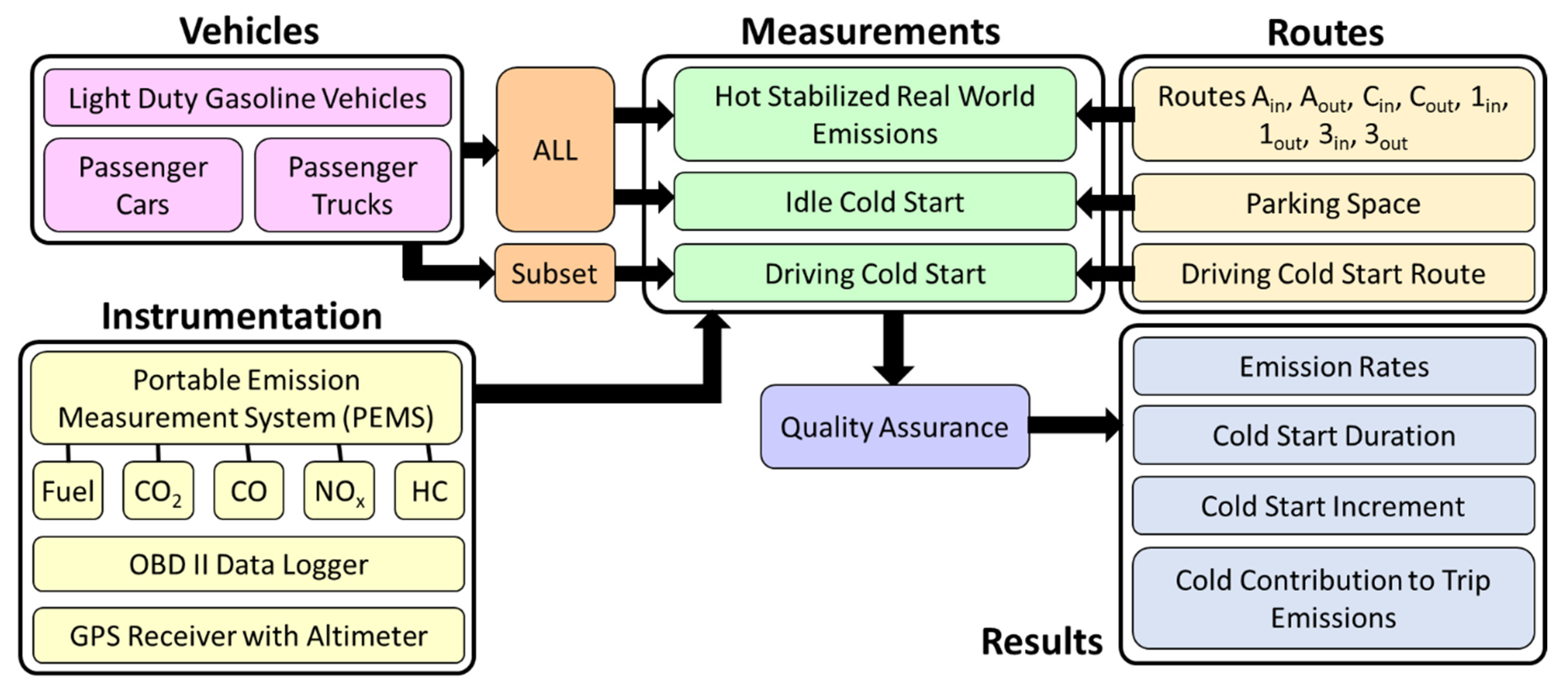
This section describes the approach used here, including (a) the design of a field study that quantifies real-world cold start duration and increment; (b) field data collection under real-world conditions; (c) data quality assurance procedure; and (d) data analyses to provide results and insights regarding the key factors motivating the study. A schematic overview of the study design is given in
Figure 1, including the types of vehicles measured, the types of measurements conducted, the instrumentation used for the measurements, the routes for which measurements were taken, the role of quality assurance, and the types of results that were produced.
2.1. Study Design
Data were collected for 37 LDGVs, including 18 passenger cars (PCs) and 19 passenger trucks (PTs). These vehicles, listed in
Table 1, include 2000 to 2016 model years, 1.4 L to 5.3 L engines, 1070 kg to 2520 kg curb weights, and 90 km to 250,000 km accumulated driving distance. For each vehicle, an idle cold start measurement was conducted. The ambient temperature ranged from −1 °C to 32 °C, and relative humidity ranged from 30% to 100%. The engine parameters and ambient conditions were compared with idle cold start duration and increment to evaluate the effect of these factors.
Table 1 also contains results data that will be addressed in the
Section 3.
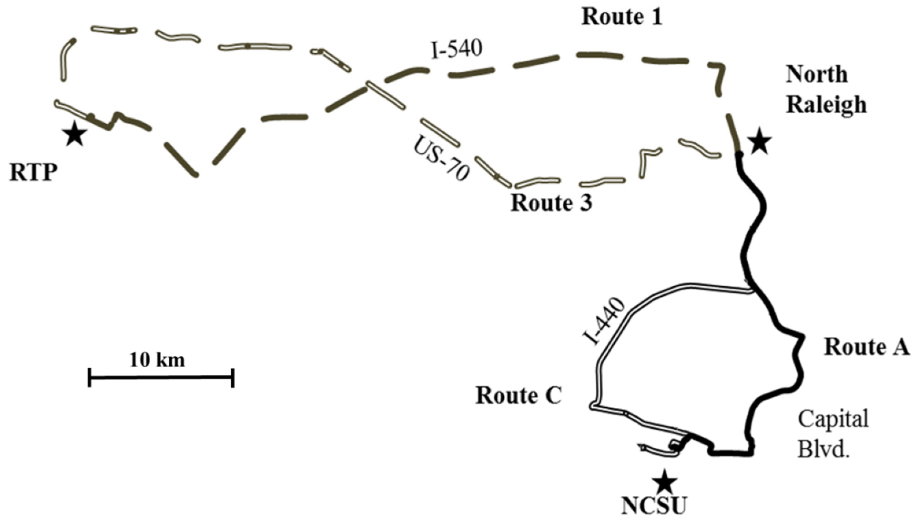
For each vehicle, a hot-stabilized running measurement was conducted for 177 km of driving on four routes in the Raleigh and Research Triangle Park (RTP) area, NC, as shown in
Figure 2, so that the cold start contribution to total trip mass emissions could be quantified. These routes have a range of road types, including feeder/collector streets, minor arterials, major arterials, freeways, and ramps, with speed limits ranging from 40 to 113 km/h. These routes were established in prior research and are analyzed as eight one-way trips [
37]. These routes represent typical commuting trips in the RTP area.
Selected characteristics of these routes are summarized in
Table 2, including route length, posted speed limits (which vary among segments within each route), the number of traffic signals, observed average speed, range of road grade, observed average relative positive acceleration (RPA), and observed average vehicle specific power (VSP). These data indicate that Routes 1 and 3 are longer than Routes A and C, that there are fewer traffic signals and higher average speeds for Routes 1 and 3 than for Routes A and C, and that average power demand (VSP) is highest for Route 1, lowest for Route A, and approximately the same at moderate values for Routes 3 and C. The average RPA is similar among many of the routes except for the relatively high value for inbound travel on Route 1. More details regarding how RPA and VSP are estimated are given by [
36].
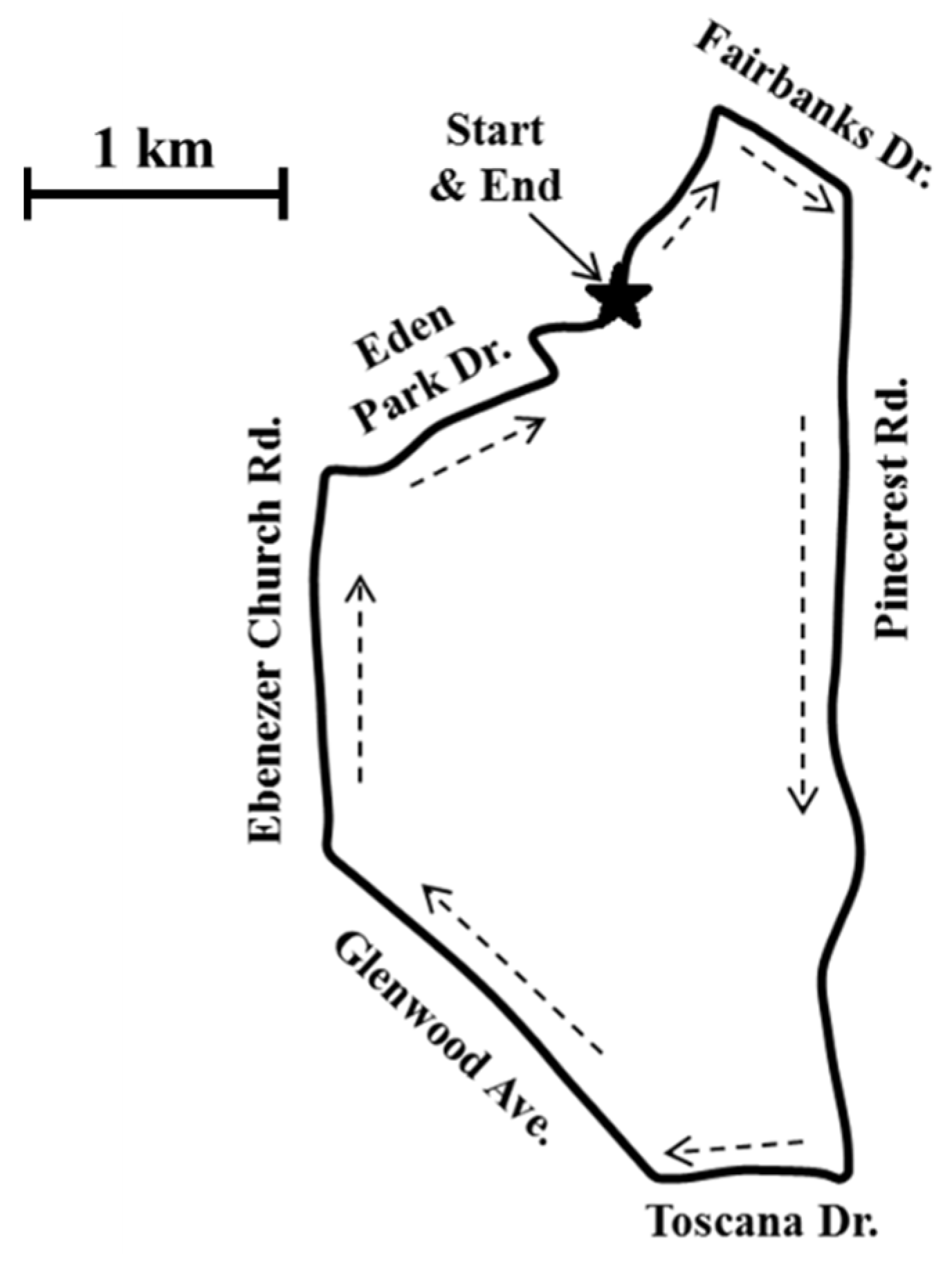
For 5 of the 37 vehicles, an additional set of measurements was conducted to characterize cold starts during driving. The number of vehicles measured for driving cold starts is less than the total number of vehicles measured because of the additional logistics involved. Cold start and hot-stabilized driving were each conducted on a 6.7 km circuit, shown in
Figure 3, comprising feeder/collector, minor arterial, and primary arterial roads with speed limits ranging from 40 to 72 km/h. The vehicles were driven on the circuit route promptly after engine start, followed by one or more hot-stabilized circuits on the same route. For a driving cold start, the vehicle has to be staged for a 12 h soak at the origin of the driving cold start route, as opposed to a parking space convenient to a vehicle owner, which leads to extra time of possession of the vehicle for measurements.
2.2. Instruments
For each vehicle, an OEM-2100 Montana or an OEM-2100 Axion PEMS was used to measure tailpipe exhaust concentrations. These PEMS, or very similar models from the same manufacturer, have been independently validated [
38,
39]. Two parallel gas analyzers measured concentrations of CO, HC, and CO
2 using non-dispersive infrared detection (NDIR), and NO and O
2 using electrochemical sensors, at 1 Hz data logging frequency. The PEMS was calibrated before measurements and zeroed during measurements [
37].
Battelle compared the exhaust concentrations between the same model PEMS and reference method instruments based on dynamometer tests [
38]. The reference methods were federal reference methods including nondispersive infrared (NDIR) for CO
2, NDIR for CO, flame ionization detector for HC, and chemiluminescence for NO
x. The cycle average emission rates for CO, NO
x, and CO
2 were within 10% between these methods. The HC emission rates from NDIR were lower than for the reference method by a factor of approximately two. This bias for HC emission rates was expected because NDIR responds well to straight-chain alkanes but not to other types of HC, whereas the reference method better characterizes total HC [
40,
41].
The HC measurements used here are for relative comparisons. Additional details on instrument performance can be found elsewhere [
33,
35,
36,
37,
42,
43,
44,
45].
An on-board diagnostic (OBD) scantool was used to record data reported by the vehicle electronic control unit (ECU), including engine speed (RPM), intake manifold absolute pressure (MAP), intake air temperature (IAT), mass airflow (MAF), mass fuel flow (MFF), vehicle speed (VSS), engine coolant temperature (ECT), catalyst temperature, ambient temperature, and barometric pressure, when available. These engine parameters were used to quantify engine activity and to estimate engine air flow or fuel flow [
43,
44]. TWC temperature could be based on a measurement from a thermocouple or could be calculated from a temperature model in the ECU. The source of the reported TWC temperature data was not reported via the OBD-II interface. However, the logged data are useful because they provide an indication of TWC temperature as reported based on the manufacturer’s preference in a manner that can be accessed by any user who logs OBD data.
2.3. Cold Start
Idle cold start measurements, for which the vehicles had a soak time of 12 h or longer, were conducted in a parking space at a location convenient to the vehicle owner. Prior to engine start, the ignition was turned to “accessory” to enable the OBD scantool to read ECU data. Once baseline ECU data were obtained, the engine was turned on, and idling was conducted for 15 min. Typically, by the end of the 15 min period, the ECT and catalyst temperatures reached a steady-state indicative of hot-stabilized operation. The driving cold start took place after a 12 h soak. The vehicle was driven immediately after the engine start.
2.4. Quality Assurance
For each of the cold start and hot-stabilized running measurements, collected data were synchronized (time aligned) and combined. Time alignment takes into account the different delay times for the exhaust sample to reach the PEMS gas analyzers compared to the time for an OBD signal, or a GPS signal, to be recorded. The combined dataset was screened for errors, and errors were corrected when possible. Typical errors, which were infrequent, included both gas analyzers zeroing simultaneously and unusual air-to-fuel ratio (AFR). Errant seconds that could not be corrected were omitted from further analysis. More details on the quality assurance procedure are given elsewhere [
43]. As shown later, cold starts take place over a period of many seconds. Prior work has demonstrated that errors in time alignment of as much as a few seconds do not substantially affect the accuracy of inferred emission rates over such time periods [
43]. The time alignment procedures are typically accurate to within one second.
2.5. Emission Rates
Emission rates were estimated at 1 Hz for cold start and hot-stabilized driving. For 26 out of 37 vehicles, the MFF was reported by the ECU. Total estimated fuel use for the hot-stabilized driving routes was compared to actual fuel consumed based on topping off the fuel tank before and after the measurement. For these vehicles, the 1 Hz exhaust flow rates were estimated based on MFF, mole fractions of CO, HC, and CO
2 in the exhaust, and the molecular weight of the fuel [
43]. For the other 11 vehicles, neither MFF nor MAF was reported. For these vehicles, the speed-density method was used to estimate MAF based on the ideal gas law, taking into account RPM, MAP, IAT, engine displacement, engine compression ratio, and volumetric efficiency (VE) [
43,
44]. VE is the ratio of actual to theoretical mass flow. AFR was inferred from the measured exhaust gas concentrations, and MFF was subsequently estimated based on MAF and AFR. VE was calibrated so that the total estimated MFF was equal to the actual fuel consumption subject to a constraint that VE is less than or equal to 0.95. The speed-density method has been verified to be accurate when compared to the direct reporting of MAF or MFF from the electronic control unit [
44]. Exhaust flow rates were estimated using MAF and MFF. For all vehicles, based on the estimated exhaust flow rate, the mole fraction of each pollutant in the exhaust, and the molecular weight for each pollutant, time-based mass emission rates were estimated [
43].
The hot-stabilized idling rates of fuel use and emissions were estimated based on the seconds when the vehicle was idling at a parking space between finishing a one-way trip and starting the next trip. The sample sizes for hot-stabilized idling were typically over 600 s for each vehicle.
2.6. Cold Start Duration and Increment
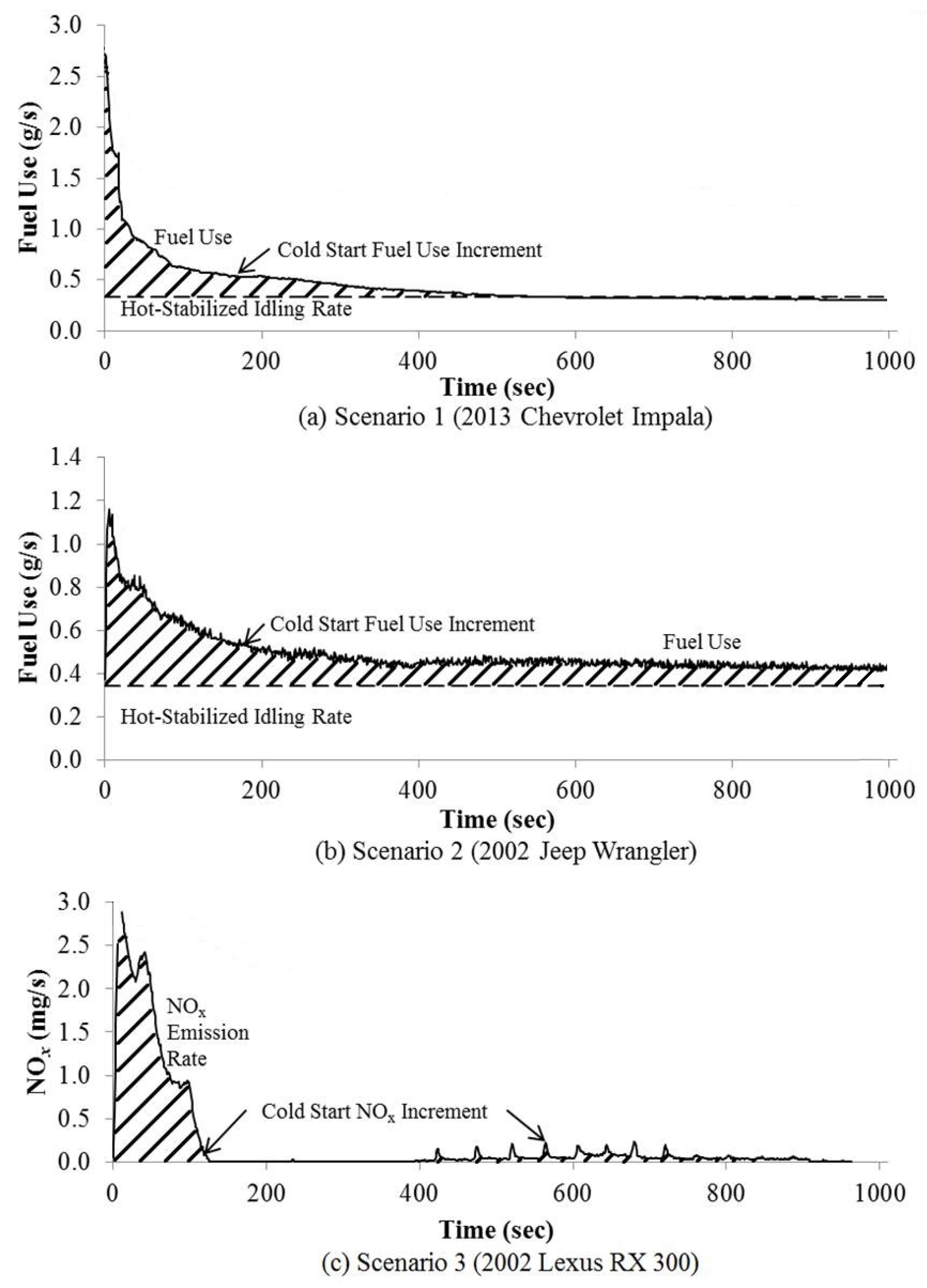
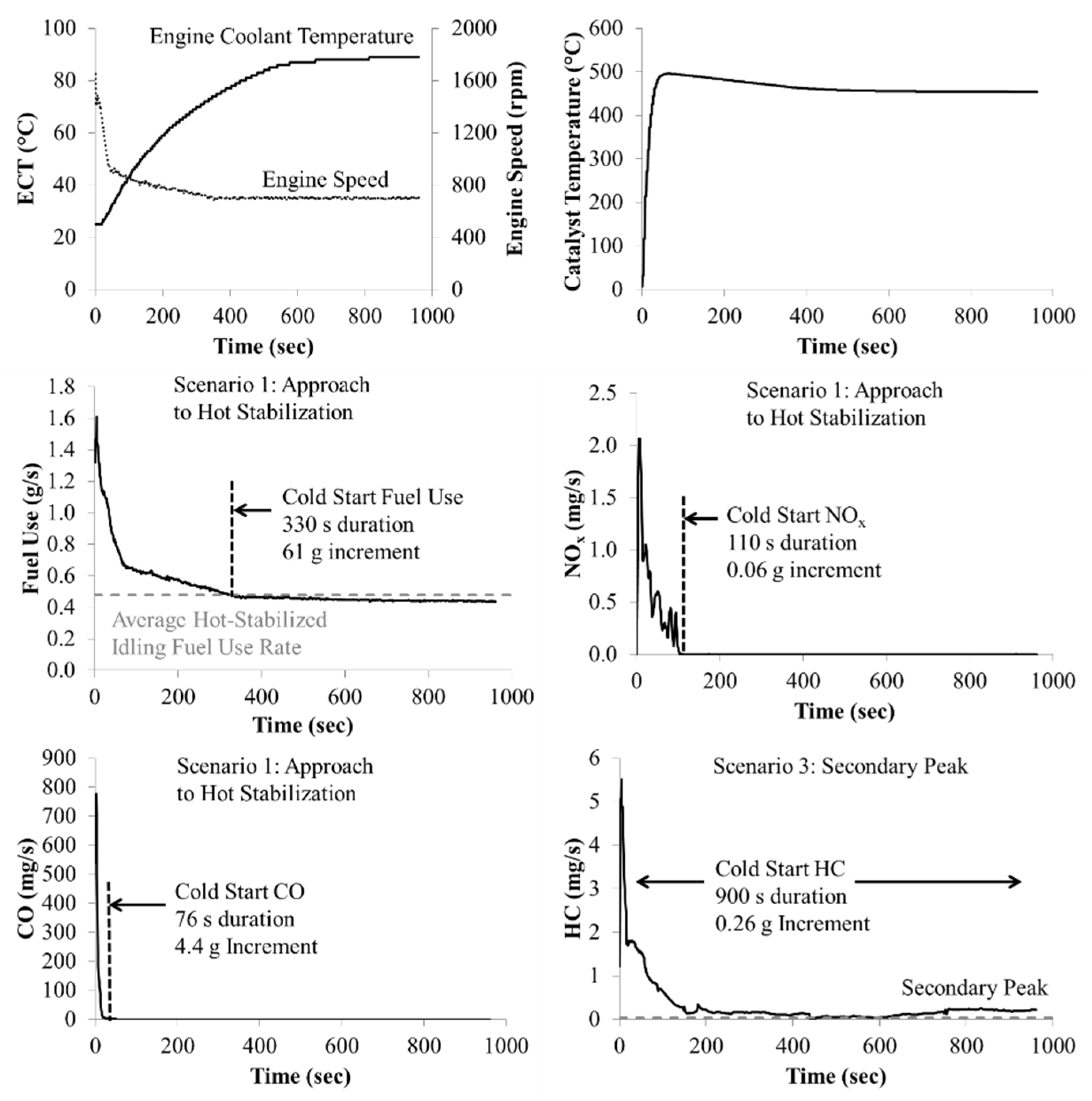
To quantify the idle cold start duration and increment for fuel use and emissions, the time-based fuel use and emission rates were compared with the average hot-stabilized idling rates for the same vehicle. Three scenarios for characterizing cold start are illustrated in
Figure 4: (1) Scenario 1—Approach to Hot Stabilization; (2) Scenario 2—Approach to Steady State; and (3) Scenario 3—Secondary Peaks. These scenarios are assigned to individual rates of fuel use and emissions for each vehicle, depending on the trends observed in the measured data.
An example of Scenario 1 is shown in
Figure 4a for fuel flow rate. Within 600 s of engine start, the fuel flow rate has reached the hot-stabilized idling rate. The cold start increment is based on integrating the area under the mass rate curve that is above the hot-stabilized idling rate to the time when the hot-stabilized idling rate is achieved. In Scenario 2, as illustrated in
Figure 4b, the fuel flow rate reaches steady-state within approximately 500 s, but the steady-state fuel use rate is higher than that measured for hot-stabilized operation. In this case, the cold start increment is estimated based on the entire 15 min measurement period, taking into account the area under the curve for measured rates less the hot-stabilized rate. Scenario 3 is based on the observation of some situations, especially for HC and NO
x, in which the initial pulse of high emission rates is succeeded by periods of very low rates followed by a secondary low frequency smaller magnitude peak, associated with transient engine operation. For example, in
Figure 4c, the first part of the cold start increment occurs within approximately 100 s, but from 400 to 950 s there are secondary peaks. The total cold start increment for Scenario 3 includes the area under both peaks, above the hot-stabilized idle emission rate. Typically, for CO, HC, and NO
x, hot-stabilized emission rates are very low compared to those observed during the cold start due to reduced engine oil and fuel viscosity, better combustion efficiency, and operation of the TWC above the light-off temperature.
For driving cold start, the cold start duration was estimated based on plots of exhaust concentrations versus distance for the driving cold start lap and driving hot-stabilized laps. At the point in time at which the exhaust concentration during the driving cold start lap appears to be the same as the driving hot-stabilized lap after possible secondary peaks, the corresponding location was designated as the end of driving cold start. The time spent in the cold start lap to reach that location was the driving cold start duration. Since the driving cold start duration for each pollutant differs, the location of the end of cold start varies by pollutant for a given vehicle. Because the cold start typically ended within the cold start lap, the difference in total pollutant mass emitted during the cold start versus subsequent hot-stabilized laps was quantified as the driving cold start increment.
2.7. Cold Start Contribution
The idle CSC for a particular pollutant and trip was estimated based on the idle cold start increment divided by the sum of the idle cold start increment and the hot-stabilized total emissions. Hot-stabilized emissions for CO, HC, NOx, and CO2 were estimated by summing the 1 Hz emission rates during a given one-way trip. In addition, the idle CSC was estimated based on all mass of fuel consumed or pollutant emitted during idling, on the assumption that all of the idling occurs before the start of trip travel activity. Similarly, driving CSC was estimated based on driving cold start increment and the hot-stabilized total emissions.
3. Results
The results include quantification of cold start duration and increment based on real-world measurements and CSCs.
3.1. Idle Cold Start Duration
An example of an idle cold start measurement is given in
Figure 5 for a 2008 Chevrolet Impala. The ECT reached a steady state in approximately ten minutes. The catalyst temperature increased rapidly within the first minute. The fuel use rate decreased monotonically to the average hot-stabilized idling fuel use rate at 331 s after engine start. The NO
x and CO emission rates each had an initial peak, and then decreased to hot-stabilized rates at 112 s and 72 s, respectively. These are categorized as Scenario 1. By contrast, for HC, the emission rates decreased over the first 400 s and then exhibited a low magnitude peak starting at 600 s. Therefore, the HC cold start increment is quantified based on Scenario 3.
For 23 of the 37 measured vehicles, the fuel use rates at the end of the 15 min are somewhat higher than the hot-stabilized fuel use rates; therefore, Scenario 2 is applied. For the other 14 vehicles, the fuel use cold start increments are quantified based on Scenario 1.
For CO, HC, and NOx emissions, the emission rates decrease to below the average hot-stabilized idling rates within 300 s for many vehicles. However, there were 10, 22, and 20 vehicles that have secondary CO, HC, and NOx peaks, respectively, and are characterized based on Scenario 3. For the remaining vehicles, Scenario 1 is applicable.
For the 37 vehicles, the average cold start durations, plus or minus 95% confidence intervals, for fuel use, CO emissions, HC emissions, and NOx emissions are approximately 690 ± 100 s, 460 ± 110 s, 680 ± 100 s, and 540 ± 130 s, respectively. Most of the idle cold start increment accrues soon after the engine start. For example, the time needed to accumulate 90% of the cold start increments, plus or minus a 95% confidence interval, for fuel use, CO emissions, HC emissions, and NOx emissions is 400 ± 80 s, 150 ± 70 s, 330 ± 100 s, and 120 ± 70 s, respectively. For CO and NOx in particular, most of the idle cold start effect occurs within approximately two to three minutes, even though the engine may not reach hot-stabilized operation for perhaps ten minutes. The results here indicate that the cold start duration differs for different pollutants and thus, the end of idle cold start needs to be determined individually for each pollutant.
For all vehicles, the idle cold start duration to accumulate 90% of the NOx cold start increment increases with vehicle mileage with a statistically significant (i.e., significantly different than zero) albeit small R2 of approximately 0.22, but is not sensitive to engine displacement, temperature, or relative humidity. For fuel use, CO, and HC, no statistically significant relationships were found for the cold start duration to accumulate 90% of the increment with respect to engine displacement, age, mileage, temperature, and relative humidity. However, there is substantial inter-vehicle variability in the cold start duration. Thus, the lack of additional statistically significant trends may be a product of sample size. A much larger sample size might yield additional insights.
3.2. Idle Cold Start Increment
Based on the data in
Figure 5, the idle cold start increments for the 2008 Chevrolet Impala are 61 g for fuel use, 4.4 g for CO emissions, and 0.06 g for NO
x emissions, each based on Scenario 1. The idle HC cold start increment, based on Scenario 3, is 0.26 g. The idle cold start increments for each of the 37 measured vehicles are given in
Table 1. For all vehicles, the average idle cold start increments for fuel use, CO, HC, and NO
x are 77 ± 13 g, 7.9 ± 3.8 g, 0.60 ± 0.20 g, and 0.16 ± 0.14 g, respectively. The results indicate that real-world idle cold start emits the same magnitude of emissions as the previously reported dynamometer cold start increments at moderate ambient temperature [
6,
13,
24].
The measured PTs have on average an approximately 28% higher fuel use idle cold start increment than the measured PCs, but the difference is not statistically significant because of large variability and limited sample size. There is no statistically significant difference between PTs and PCs in idle cold start emission increments for CO, HC, NOx, and CO2.
The idle cold start fuel use increments increased as ambient temperature decreased (R
2 = 0.25), for which the R
2 value is statistically significantly different than zero but is small in magnitude, but is not statistically significantly correlated with engine displacement, age, mileage, or relative humidity. Idle cold start HC increments significantly increase with increasing engine displacement (R
2 = 0.23) but are not sensitive to mileage or ambient conditions. Idle cold start CO and NO
x increments significantly increase with increasing mileage (R
2 = 0.24 and 0.19, respectively) and decrease with ambient temperature (R
2 = 0.33 and 0.09, respectively), but are not significantly sensitive to engine displacement or relative humidity. The very weak trend with regard to ambient temperature for NO
x versus CO is consistent with other studies that have found that CO emissions increase with decreasing ambient temperature, but NO
x emissions can, in some cases, decrease with decreasing ambient temperature [
16]. Overall, trends in these significant relationships with ambient temperature agree with previous studies for similar temperature ranges [
6,
13]. For example, Gao et al. [
22] reported that initial engine temperature (which is approximately the same as ambient temperature) has a “great impact” on emission rates during a cold start. However, the relationship between cold start increments and ambient temperature may be more sensitive for lower temperatures than observed here [
6]. The key factors that affect the idle cold start increments of fuel use and emissions of particular pollutants may differ.
3.3. Driving versus Idling
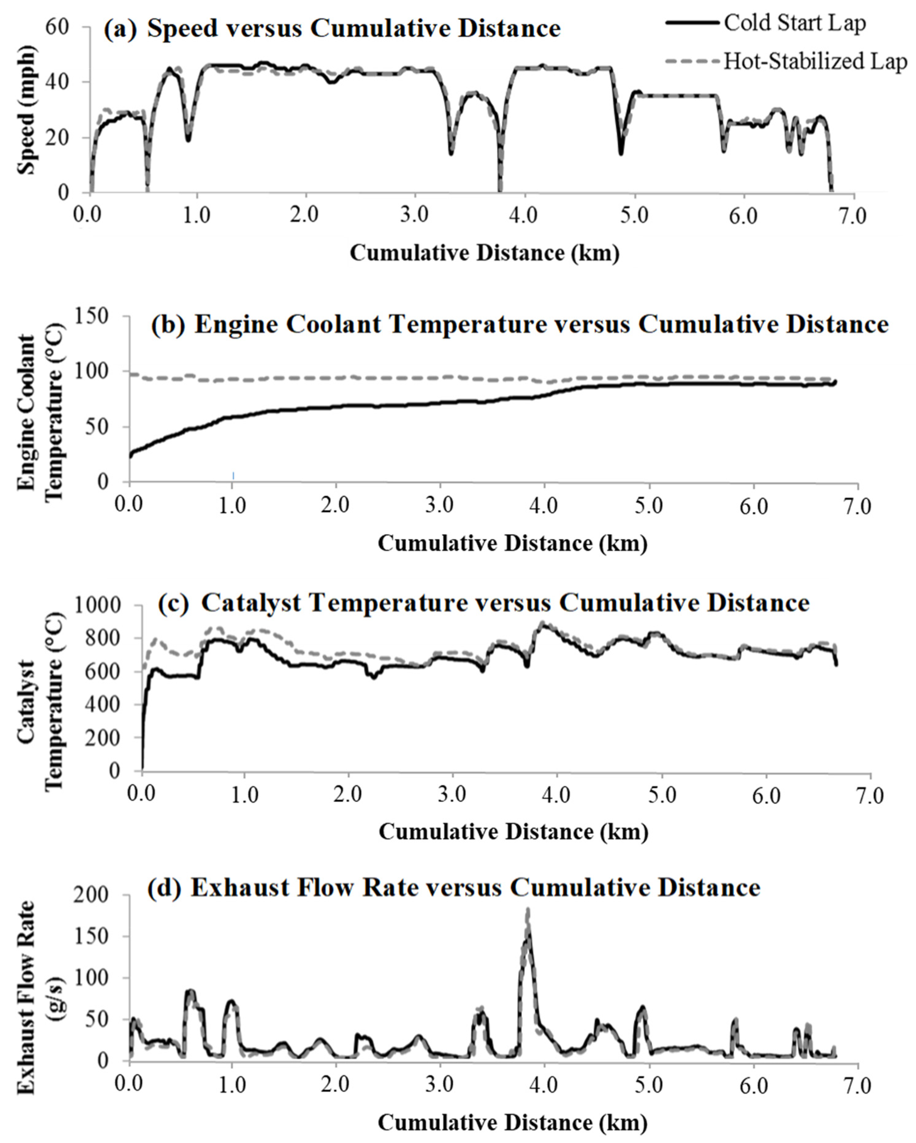
An example result for the comparison of cold start and hot-stabilized vehicle operation during driving is given in
Figure 6 for the 2015 Ford Fusion.
Figure 6a demonstrates that the speed versus cumulative distance trace was repeatable between the cold start lap and the hot-stabilized lap. The vehicle was driven on both laps by the same driver. Based on local knowledge of the terrain, road type, speed limits, and locations of landmarks, the driver operated the vehicle to achieve specific speeds at specific locations on each lap. For example, the driver operated the vehicle to reach the posted speed limit of 72 kph on Fairbanks Drive at the first hill crest (at approximately 0.7 km cumulative distance), and to reach a speed of 32 kph for the turn from Fairbanks Drive onto Pinecrest Road (at approximately 0.9 km cumulative distance).
Figure 6b illustrates that the engine coolant temperature gradually rose from ambient temperature to hot-stabilized steady-state during the first 4.8 km of the cold start lap, and that the engine coolant temperature was approximately at steady state during the warm stabilized lap.
Figure 6c illustrates that the TWC was initially very low during the cold start lap. Although the TWC temperature rose quickly during the first 0.16 km of cold start operation, it did not reach hot-stabilized temperature levels until approximately 3.2 km into the cold start lap.
Figure 6d illustrates that the estimated engine exhaust flow rate followed the same peaks for both cold start and hot-stabilized laps, which is indicative of the similarity of the speed traces for both laps.
Driving cold start durations and increments are summarized in
Table 1. For CO, HC, and NO
x, the average driving cold start durations are approximately 152 ± 130 s, 290 ± 210 s, and 93 ± 52 s, respectively. These are shorter than the idle cold start durations by 74%, 61%, and 61% for CO, HC, and NO
x, respectively. Similar to the idle cold start results, the driving cold start results imply that cold start durations can be different for different pollutants. Such differences can affect the location and intensity of on-road emissions as the vehicle is driven, leading to heterogeneity in near-road air quality and exposure to traffic-related pollutants. The data suggest that driving leads to shorter cold start duration compared to idling. It was not possible to clearly determine the cold start durations for fuel use or CO
2 emissions, because these rates did not differ substantially on a 1 Hz basis compared to rates observed during hot-stabilized driving.
Emissions during the cold start lap significantly exceed those during the hot-stabilized laps. The average circuit total CO emissions were 340% higher for a cold start than for hot-stabilized driving, based mostly on 320% higher average exhaust concentration in combination with a 10% higher average exhaust flow rate. The travel times for cold start and hot-stabilized laps were within 2% and thus are not a significant source of variability. Similarly, the circuit total HC and NOx emissions averaged 9.2 times and 3.9 times, respectively, higher for cold start versus hot-stabilized driving, influenced mostly by corresponding higher exhaust concentrations with a small impact from the increased exhaust flow rate.
Driving cold start increments were estimated and summarized in
Table 1. On average, for the five measured vehicles, the driving cold start increments are higher than the idle cold start increments by a factor of 4 with an inter-vehicle range of 0.9 to 25 for CO, a factor of 2.1 with an inter-vehicle range of 0.1 to 3.6 for HC, and a factor of 10.2 with an inter-vehicle range of 5.0 to 85 for NO
x. Thus, although inter-vehicle variability exists, the driving cold start increments are found to be substantially higher, on average, than for idle cold start increments. In addition, the average exhaust flow rates during the driving cold starts for the five vehicles are five times higher than for the idling cold starts. Therefore, the idle cold start increments may be a practical lower bound on real-world cold start increments. Moreover, driving cold starts could substantially contribute to near-road air quality concentrations and to human exposure to air pollution in the vicinity of roads that are affected by cold starts.
An idling vehicle does not provide any useful transportation service. Thus, the entire accumulated emissions during an idle cold start represent an incremental contribution to emissions associated with idling prior to the start of a trip. Therefore, when comparing a cold start for idling versus driving, the entire emissions during idling could be compared to the cold start increment during driving. The total fuel use and CO2 emissions for the 15 min idling period averaged approximately 4 times higher than for the driving cold start increment, with an inter-vehicle range of approximately 2 to 10 times. The idling cold start CO, HC, and NOx total emissions, on average, were substantially lower than the driving cold start increments by approximately 70%, 45%, and 90%, respectively. Therefore, idling after engine start leads to higher fuel use and CO2 emissions but lower average CO, HC, and NOx emissions compared to driving cold start. Overall, driving during the cold start leads to the highest cold start CO, HC, and NOx emissions of the cold start cases considered.
As a sensitivity test case, a measurement was made for a “five and drive” scenario for one vehicle, the 2014 Ford Fusion, in which the vehicle was idled for 5 min and then driven on the driving cold start circuit. The purpose of this case was to evaluate whether some idling prior to driving would help reduce the cold start emissions, given that the driving cold start emissions for CO, HC, and NOx are very high. Based on comparing the total emissions during the five minutes of idling and the increment during driving, the “five and drive” case had approximately half the CO, a third of the HC, and a quarter of the NOx emissions compared to the driving case. However, because of the five minutes of no driving, the total fuel use and CO2 emissions attributed to the start during the “five and drive” case were approximately twice as high as for driving. Thus, a hybrid start strategy of idling followed by driving can help reduce exhaust emissions of some pollutants, with the tradeoff of more fuel consumption and higher greenhouse gas emissions.
3.4. Cold Start Contribution
To illustrate the contribution of an idle cold start to total trip emissions, details are given in
Table 3 for the 2008 Chevrolet Impala. The CO idle cold start increment was 4.4 g. For Route A-Out, the trip-total CO emissions were 9.1 g. Thus, the total emissions with a cold start increment would be 13.5 g, of which 33% is the cold start contribution. On average, over eight trips, the CO CSC is 18%. The trip-specific estimated CSCs vary from 12% to 36% for CO, from 37% to 74% for HC, from 6% to 22% for NO
x, and from 2.6% to 4.3% for CO
2, depending on the one-way route. Typically, over 99% of the carbon content in the fuel is converted to CO
2; therefore, the trends in fuel use and in CO
2 emissions are essentially the same.
Trip fuel use and emissions are estimated per methods detailed elsewhere [
35,
36], that in turn are based on the estimation of mass flows of fuel, air, and exhaust through the engine. These estimates have been validated by comparing estimated fuel consumption to actual fuel consumption. Khan and Frey [
45] reported that the average estimated fuel use for the methods employed here is 98 ± 2% of actual fuel use. As shown in the
Supporting Material, the average estimated trip fuel use for 36 of the 37 vehicles is within 1.8% of the actual fuel use, which indicates accuracy. For one vehicle, actual fuel use was not available. The engine mass throughput estimates are an accurate basis for estimating emission rates.
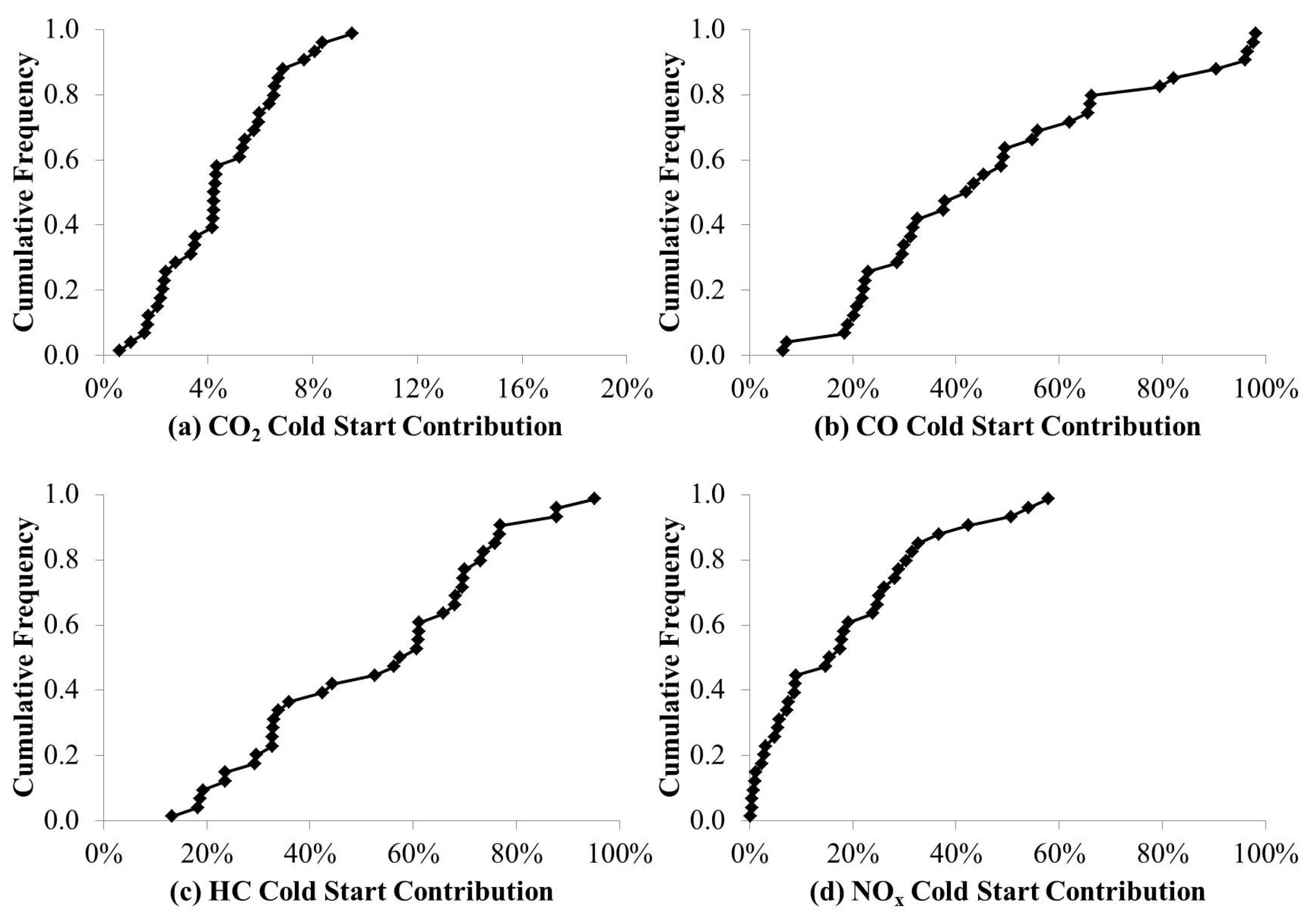
Figure 7 shows the cumulative distribution functions (CDFs) of inter-vehicle variability in estimated idle CSCs averaged over eight trips for each of the 37 measured vehicles. Thus, each data point represents one vehicle and the average of CSC for Routes A
in, A
out, C
in, C
out, 1
in, 1
out, 3
in, and 3
out. For 35% and 57% of vehicles, the CO and HC, respectively, idle CSCs comprise over 50% of trip emissions. For NO
x, idle CSCs range from approximately 0 to 60%. On average, the idle CSC for CO is 47%, with a 95% confidence interval on the mean of ±10%. The 95% confidence interval for the mean takes into account inter-vehicle variability in the CSC and the sample size and is indicative of the precision of the mean estimate. On average, the idle CSCs for HC, NO
x, and CO
2 are 52 ± 8%, 18 ± 6%, and 4.5 ± 0.8%, respectively. The data provide evidence that approximately half of the trip total CO and HC and one-fifth of the trip total NO
x come from an idle cold start for a trip of 16 to 27 km. Since a significant portion of trip total emissions comes from a cold start, the results demonstrate the necessity for future research that focuses on reducing cold start emissions. These estimates also illustrate that mean CSC can be estimated with high precision for CO
2 based on a relatively small sample (37 vehicles), and that the mean CSCs for the other pollutants can be estimated with a precision of within plus or minus 10 percent with such a sample. Of course, the CSC estimates are specific to the routes being analyzed.
For all measured vehicles, there is inter-trip variability in observed idle CSCs. One key reason for the variability is trip distance. For example, for CO2, the idle CSCs are typically the highest for Routes A and C, since there are fewer trip total CO2 emissions due to shorter distances compared to other routes. By contrast, Route 3 has the longest distance and typically the highest total trip CO2 emissions, resulting in the lowest CO2 CSCs. For CO, HC, and NOx, similar trends are observed, with Routes A and C typically having higher CSCs than other routes and Route 3 having lower CSCs than other routes.
If all of the fuel use and emissions during idling, prior to a trip, are attributed to a cold start, the CSCs are higher for fuel use and CO2 but essentially unchanged for the other pollutants. The average CSCs based on the total mass of each pollutant emitted during idling are 48 ± 9%, 55 ± 7%, 19 ± 6%, and 16 ± 1% for CO, HC, NOx, and CO2, respectively. The ranges given are 95% confidence intervals of the mean estimate based on inter-vehicle variability with a sample size of n = 37. These CSCs for CO, HC, and NOx are essentially the same as those estimated based on only the incremental mass emitted above the hot-stabilized rate. However, the CO2 CSCs based on totals are significantly higher than the ones based on increments.
The idle CSCs based on idle cold start increment decrease significantly with increasing ambient temperature for CO, HC, and CO2. For NOx, a decrease is observed but it is not statistically significant. For idle CSC versus the other factors, such as engine displacement, vehicle model year, vehicle mileage, and relative humidity, no statistically significant trends are observed.
For driving cold start, the average driving CSCs were 61 ± 33%, 62 ± 33%, 56 ± 30%, and 4.2 ± 2.5% for CO, HC, NOx, and CO2, respectively, for the five vehicles for which driving cold starts were measured. The ranges given are 95% confidence intervals for the mean taking into account inter-vehicle variability based on a sample of five vehicles. The ranges of the confidence intervals of these mean values are larger than those based on idle cold starts because of a smaller sample size (n = 5 for driving cold starts versus n = 37 based on idle cold starts). The confidence intervals for the mean are indicative of the precision of the mean estimate. These confidence intervals could be narrowed by collecting data on a larger vehicle sample. The mean estimates indicate that driving cold start likely yields substantially higher CSCs for CO, HC, and NOx, compared to an idle cold start. For CO2, the driving CSCs are similar to those based on idle cold start increments but significantly lower than for those based on idle cold start totals.
4. Discussion
Idling was used for all vehicles as the basis for measuring cold starts because it controls all measured vehicles to the same operating condition after engine start. The effect of driving versus idling after a cold start for five vehicles shows that driving typically leads to substantial increases in the cold start increment for CO, HC, and NOx. When measuring driving cold starts, there is some variation in traffic-induced delay between cold start and hot-stabilized laps, which can be reduced depending on the time of day and day of the week when the circuit is driven. It was possible to obtain repeatable vehicle activity on a real-world driving circuit from which real-world driving cold start increments could be inferred. While the repeatability of the driving cold start measurements was indicated by the consistency of speed versus distance traces for cold start and hot-stabilized laps, future work could repeat the experience for individual vehicles to assess the consistency of inferred cold start duration and increment. Furthermore, the methodological approach illustrated here to measure driving cold start should be expanded to a larger vehicle sample.
Future work could consider whether some of the variability in cold start emissions increments can be attributable to differences in TWC layout and specification, including whether the TWC is close-coupled to the engine or located farther downstream of the engine under the vehicle floor, or whether the TWC has a uniform or zone-structured catalyst loading.
An idle cold start could last beyond 15 min, but most of the emissions occur during the first 2 min, approximately, for CO and NOx and 5 min for HC. Thus, cold start duration differs among pollutants. Driving substantially decreases cold start duration. Furthermore, exhaust emissions during driving were elevated for typically the first 0.16 to 3.22 km after a cold start, indicating that the impact of cold starts would not be localized only to the parked location of the vehicle but would be distributed onto the road network in the vicinity of cold starts. More detail on the timing and location of cold start emissions can improve estimates of near-road air quality and exposure affected by such emissions.
Using modeled emission rates based on measured vehicle trajectories, Jiang et al. [
4] estimated that pedestrian, bus passenger at bus stops, and cyclist CO exposures are underestimated by 67% to 89% if cold-start emissions are neglected. The accuracy of these estimates could be refined by measuring, rather than modeling, cold start emissions.
Furthermore, cold start emissions contribute to human exposure to traffic-related emissions in parking garages. For example, Liu and Zimmerman [
46] found, based on measurements with low-cost sensors, that vehicle NO
x and CO emissions in selected work location parking garages averaged approximately 10 to 50 percent higher, respectively, in the evening than in the morning. In the morning, the vehicles entered the garage in hot-stabilized operating mode at the end of the morning commute trip. In the evening, the vehicles were started in the garage after a soak time equivalent to the time that the driver was at the work location, which would typically be eight or more hours. Thus, the evening vehicle starts were typically cold starts.
In terms of cold start increment, compared between idling and driving, higher fuel use and emissions are observed for driving cold start. The pilot “five and drive” scenario provides some evidence that idling for 5 min can substantially reduce cold start emissions of CO, HC, and NO
x but increase energy use compared to driving. Therefore, the results give some insight regarding the potential of reducing cold start emissions via operational practices. However, there is a surprising scarcity of data upon which to develop rigorous advice regarding how drivers can best reduce their own cold start emissions. Furthermore, the results vary from one vehicle to another. Therefore, data for additional vehicles and for additional cold start scenarios (e.g., different combinations of idling and driving) are needed. Furthermore, data are needed for primary particulate matter emissions. For example, the market share of gas direct injection (GDI) vehicles is growing in the U.S. GDI vehicle cold start emissions may differ for NO
x, particle number, and soot mass emissions [
17,
19,
47].
A cold start contributes a significant portion of trip total emissions. The CSCs depend on driving versus idling, pollutant, trip distance, ambient conditions, and driving cycles, but were found here to not be sensitive to engine displacement, vehicle model year, vehicle mileage, or relative humidity. The latter lack of significant findings does not imply that these factors may not be of importance. Rather, the potential role of such factors may be masked by the high inherent inter-vehicle variability in the data and would require a much larger sample size to detect with significance. Furthermore, although it is known that engine soak time is a key factor that affects cold start emissions, variability in soak time was not part of this study. Assessment of variability in soak time requires control of the vehicle for a much longer time period than was possible here, given that most of the vehicles were contributed voluntarily by drivers without financial compensation, and should be considered in future work.
This research focused on LDGVs with internal combustion engines (ICEs) and conventional power trains. Cold starts also occur for hybrid electric vehicles (HEV) and for plug-in hybrid electric vehicles (PHEVs) which also have ICEs [
48]. The first engine start after a 12 h soak for either an HEV or a PHEV could occur some distance from the origin of a trip, depending on the state of charge of the traction battery. Furthermore, ICE engine operations for these vehicles differ from those of conventional LDGVs. Therefore, the location, duration, and magnitude of cold starts for HEVs and PHEVs are likely to differ from the results reported here for conventional LDGVs.
Overall, this paper contributes to the state of knowledge by directly comparing incremental cold start emissions with hot-stabilized trip emissions for the same set of vehicles based on real-world measurements of in-use vehicles. The results given here confirm that cold starts are a significant contributor to total exhaust emissions from LDGVs and should motivate increased attention to their characterization.
5. Conclusions
This work focused on quantifying cold start tailpipe emissions from light-duty gasoline vehicles with three-way catalysts. Cold start duration was quantified based on idle and driving cold starts using portable emission measurement systems (PEMS). For idling cold starts, inference of cold start duration considered the time duration to reach a hot-stabilized rate, steady state, or the cessation of secondary peaks. Secondary peaks were observed for CO, HC, and NOx cold start emissions. Idle cold starts were highly variable by vehicle and by pollutant. The idle cold start durations were as short as 18 s and as long as 15 min, depending on the vehicle and pollutant. Furthermore, for a given vehicle, the cold start durations differed by pollutant. However, even though the idle cold start durations averaged from 460 s to 690 s depending on the pollutant, 90% of the cold start emissions accumulated within 120 s to 400 s, depending on the pollutant.
The cold start increments from idle cold starts were also variable by vehicle and pollutant. On average, they were comparable to values reported by others based on dynamometer measurements at moderate ambient temperatures. There were few statistically significant trends of cold start duration or cold start increment with respect to vehicle type (passenger car versus passenger truck), ambient temperature, engine displacement, vehicle age, accumulated mileage, or relative humidity. The lack of statistically significant trends in such cases is because of the large amount of variability in the results for individual vehicles and pollutants. Larger sample sizes would be needed to obtain statistically significant findings. In some cases, weak statistically significant trends were found, such as for cold start fuel increment and ambient temperature, CO and NOx cold start increments, and accumulated mileage and ambient temperature. In such cases, the observed trends were consistent with other studies based on different measurement methods and test situations.
The measurement of driving cold starts is resource-intensive because of the need to control a vehicle for a 12 h soak period, and is challenging because of the need to reproduce a driving cycle for both cold start and hot start vehicle operation in the context of a real-world test route that can be confounded by variable traffic. Nonetheless, a method for the measurement and inference of driving cold start duration and increment was successfully demonstrated, including the ability to obtain highly similar speed traces on repeated laps of the same test circuit on public roads. The driving cold start measurements were made for a subsample of 5 of the 37 vehicles for which idle cold starts were measured. The results indicate that driving during a cold start leads to shorter average cold start duration, but larger average cold start increments, than idling. Idling cold starts are much easier to measure. The comparison of driving versus idling cold starts for the subsample of five vehicles indicates that cold starts measured during idling would be a lower bound on real-world cold starts associated with driving. For one vehicle, a “five and drive” scenario was measured, in which the vehicle was idled for 5 (instead of 15) minutes prior to driving; the CO, HC, and NOx emissions from this hybrid cold start approach were lower than for a driving cold start in which the vehicle was driving immediately upon engine start although the fuel use and CO2 emissions were higher. Given the variety of real-world cold start scenarios that represent different durations of idling until the initial start of driving, additional work could be conducted following the precedent established here for measuring such scenarios.
Cold starts are potentially significant because they lead to localized emissions either at the point of vehicle engine start or over the distance driven by a vehicle while it is in the cold start phase, which affects localized near-road air quality and human and ecological exposure to such pollution. In addition, as hot-stabilized tailpipe emissions are subject to increasingly stringent regulations, cold starts are expected to contribute an increasing share to total trip-based emission rates. Cold start contributions were quantified based on several real-world routes that represent a range of road types and driving conditions typical of commuting trips in the Raleigh and Research Triangle Park area of North Carolina. The results illustrate that there is inter-vehicle and inter-pollutant variability in the CSC, and that CSC is likely be sensitive to factors such as trip distance.
In general, the sample sizes for vehicles and routes in this work were suitable for demonstrating methodological approaches, but would need to be expanded substantially in future work to allow for the identification of statistically significant relationships with factors that are expected to be associated with cold start duration, cold start increment, and cold start contribution. Nonetheless, the results robustly demonstrate that cold starts contribute a substantial share of trip emissions, providing insights into the duration and magnitude of cold start emissions. Furthermore, this work provides a framework that can support the targeted development and testing of hypotheses for evaluation in future work via augmentation with a larger sample of vehicles.


