Article

WRF Physics Ensemble Performance Evaluation over Continental and Coastal Regions in Germany

by
Ioannis Stergiou
1,
Efthimios Tagaris
2 and
Rafaella-Eleni P. Sotiropoulou
1,*
1
Department of Mechanical Engineering, University of Western Macedonia, 50100 Kozani, Greece
2
Department of Chemical Engineering, University of Western Macedonia, 50100 Kozani, Greece
*
Author to whom correspondence should be addressed.
Atmosphere 2023, 14(1), 17; https://doi.org/10.3390/atmos14010017
Submission received: 30 November 2022 / Revised: 18 December 2022 / Accepted: 19 December 2022 / Published: 22 December 2022
(This article belongs to the Special Issue Feature Papers in Atmosphere Science)

Abstract

:
WRF is used to simulate eight extreme precipitation events that occurred over the regions of Schleswig–Holstein and Baden–Wurttemberg in Germany. The events were chosen from the German Weather Service (DWD) catalog and exceeded the DWD’s warning level 3 (i.e., rainfall > 40 mm/h). A two-way nesting approach is used with 9 and 3 km spatial resolutions. Initial and boundary conditions are obtained from the ERA5 dataset at 0.25° × 0.25°. To model each event, thirty different parameterization configurations were used, accounting for all possible combinations of five microphysics (MP), three cumulus (CU), and two planetary boundary layer (PBL) parameterization methods, yielding a total of 240 simulations. TOPSIS multicriteria analysis technique is employed to determine the performance skill of each setup and rank them, using six categorical and five statistical metrics. Resolution increase from 9 to 3 km did not improve forecasting accuracy temporally or in intensity. According to TOPSIS ranking, when treating each event individually, the ideal parameterizations combination is spatiotemporally dependent, with certain members ranking higher. When all events are considered, the Morrison double-moment MP–Grell–Freitas CU–YSU PBL combination works best with a frequency of occurrence in the top five performing scenarios of 30%, 47.5%, and 57.5% respectively.

1. Introduction

Weather and climatic extremes are influenced by climate change. Evidence of observed changes in extremes such as heat waves, heavy precipitation, droughts, tropical cyclones, and their attribution to human activity [1], is constantly increasing. Heavy precipitation events are becoming more frequent and severe, and climate change is most certainly the dominant driver [1]. Increased land evapotranspiration paired with higher temperatures in a warmer climate lead to a rise in agricultural and ecological droughts, and an enhancement in the air’s capacity to hold water vapor [1,2,3,4,5], raising the likelihood of intense precipitation events. The change+ in the atmosphere’s water-holding capacity for the mid-latitudes, regulated by the Clausius–Clapeyron equation, increases by roughly 7% K−1 of temperature rise [6,7]. Given that variations in relative humidity are minimal, owing to precipitation physics, the change in the atmosphere’s water-holding capacity is translated into a similar actual rise in the air moisture content, thus increasing the rainfall intensity at about the same rate or even more, because of the enhanced moisture convergence [6,8]. As a result, global warming is more likely to aggravate subdaily precipitation extremes than daily or extended period intense events [6,9,10,11,12,13,14,15], which has already been witnessed in the new ERA5 reanalysis dataset [16].
Complex terrain, land-use diversity, and closeness to the sea are among the primary geophysical components influencing local and synoptic-scale meteorology, while playing at the same time a vital role in the interactions between the sea, land, and atmosphere [17,18,19,20,21]. In regions with such characteristics, the forecast of spatial and temporal fluctuations of intense precipitation events is a perplexing task. Predicting flash or fluvial floods is of crucial importance and heavily depends on short-term forecasting of fluctuations in the subdaily extremes. As a result, the precise forecast of heavy rainfall at subdaily time periods is a critical component of an early warning system. The combination of proper initial and lateral boundary conditions with model physical schemes setup in simulations that permit convection (i.e., those with a grid resolution less than 4 km) using Numerical Weather Prediction (NWP) models, provides tremendous promise for enhanced precipitation forecasts [22,23,24,25,26,27,28,29,30]. The adoption of fine resolution in simulations carried out by global NWP models is of crucial importance in term of forecasting, particularly in areas with a high heterogeneity in the lateral boundaries [31,32,33,34,35].
The Weather Research and Forecasting (WRF) [36,37,38] model is widely used for atmospheric research and operational forecasting, and it is among the state-of-the-art convection-permitting NWP models predicting changes in meteorological events by downscaling large-scale data. WRF is highly modular, equipped with numerous parameterization choices. However, choosing the best performing combination of parameterization schemes is difficult, as their performance highly depends on space and time. To determine the best parameterization combination, a multicriteria decision analysis method is often employed. The Technique for Order Preference by Similarity to the Ideal Solution (TOPSIS) method has been used in several studies. TOPSIS was initially introduced by Hwang and Yoon [39] and was further improved by Yoon [40] and Hwang et al. [41]. It ranks the alternatives based on their distances from the ideal and the negative ideal solution, with the best alternative having the shortest distance from the ideal solution and the longest from the worst one. TOPSIS is a compensatory aggregation technique for comparing a set of alternatives by determining weight values for each criterion, normalizing their rating, and assessing the geometric distance among each alternative and the ideal one, i.e., the one with the highest score in each criterion. For precipitation, the determinant physical parameterization schemes are the microphysics (MP), the cumulus (CU) and the planetary boundary layer (PBL) schemes, but their relative importance strongly depends on the geographical location.
Recent studies have yielded mixed results regarding extreme precipitation. Duzenli et al. [42] studied four different extreme precipitation events over two regions in Turkey, considering four MP, three CU, two PBL schemes, and evaluated the forecast skill of the simulations using the TOPSIS method. Their results do not indicate a superior combination of parameterizations that will produce the best results in all cases, as the optimal choices were spatial and seasonal dependent. Liu et al. [43] used the WRF model to assess intense rainfall events at fine spatiotemporal resolution centered over Alexandria, Egypt. They considered three microphysics (MP), three cumulus (CU) and two planetary boundary layer (PBL) schemes and quantified the simulation performances with the TOPSIS technique. The configuration they suggested comprises the WRF Single–Moment 6–Class (WSM6) [44] microphysics (MP) scheme, the Mellor–Yamada–Janjic (MYJ) [45] planetary boundary layer (PBL) scheme, and the Grell–Freitas (GF) [46,47] cumulus (CU) scheme, also pointing out the significance of using an adequate spin-up time (>12 h). Wang et al. [48] aimed to find the optimal set-up to produce the High Asia Refined v2 analysis using various MP, CU, PLB, and land-surface model (LSM) schemes. Using the TOPSIS method, they identified and concluded that a combination of the Kain–Fritsch (KF) [49] CU scheme, Morrison 2-Moment (MDM) scheme [50], Yonsei University (YU) scheme [51], and Noah [52] LSM provided the best performing one concerning precipitation. Umer et al. [53] simulated an extreme precipitation event causing floods over Kampala, Uganda. They conducted 24 simulations, combining 8 MP, 4 CU, and 3 PBL schemes, concluding with an optimum combination with the help of the TOPSIS technique. Their best MP–CU–PBL scheme combinations were the MDM–GF–ACM2 (the Asymmetrical Convective Model version 2 [54] PBL), the WSM6–KF–BL (the Bougeault–Lacarrere scheme (BL) [55]), and the WSM3 (WRF Single–Moment 3–Class [56])–KF–BL. They also noted the fact these high-performing parameterization combinations are suitable just for the specific event, pointing out the spatial dependency of the procedure. Sikder and Hossain [57], conducted a sensitivity study over Indian river basins that are monsoon governed. They also used TOPSIS to identify the top performing set of MP and CU schemes, and spatial resolutions from a total set of 15 combinations. The MP–CU scheme combination of WRF Single–Moment 5–Class scheme (WSM5)–Betts–Miller–Janjic scheme [45] (BMJ) performed best, followed by WRF Single–Moment 6–Class scheme (WSM6) [44]–BMJ and Thompson MP scheme (TS) [58]–BMJ. The difference in performance between 27 and 9 km was small, indicating that computational efficiency at 27 km may be achieved without losing precision. Additionally, raising the resolution to a finer 3 km resolution without the use of CU schemes did not improve the results. Goodarzi et al. [59] projected severe precipitation with the WRF model in Kan Basin, Iran, utilizing five distinct cumulus schemes and the TOPSIS algorithm to make flood warning decisions, concluding that the KF CU scheme can simulate convective precipitation more accurately.
In all the aforementioned studies, the spatial but also the temporal dependence of the model’s performance is emphasized, as well as the successful use of the TOPSIS technique in finding the optimal combination of parameterizations. Given that, identifying the optimal parameterization combination and assessing this capability of such a model in forecasting extreme events is vital for an early warning system and of particular interest. To address the concerns raised, this work performs a sensitivity assessment of physical schemes and spatial resolution, setting up members of the WRF model that are able to replicate chosen severe precipitation occurrences. Using a nesting approach (9 km for the parent domain and 3 km for the nested domains), five MP, three CU, and two PBL parameterization schemes are combined and evaluated over two German regions, where there are a vast number of meteorological stations (1046) and a fully embedded and freely accessible database of recorded measurements. Using the TOPSIS technique, the success of each simulation combination is ranked. The effects of model physics on WRF results are compared.

2. Materials and Methods

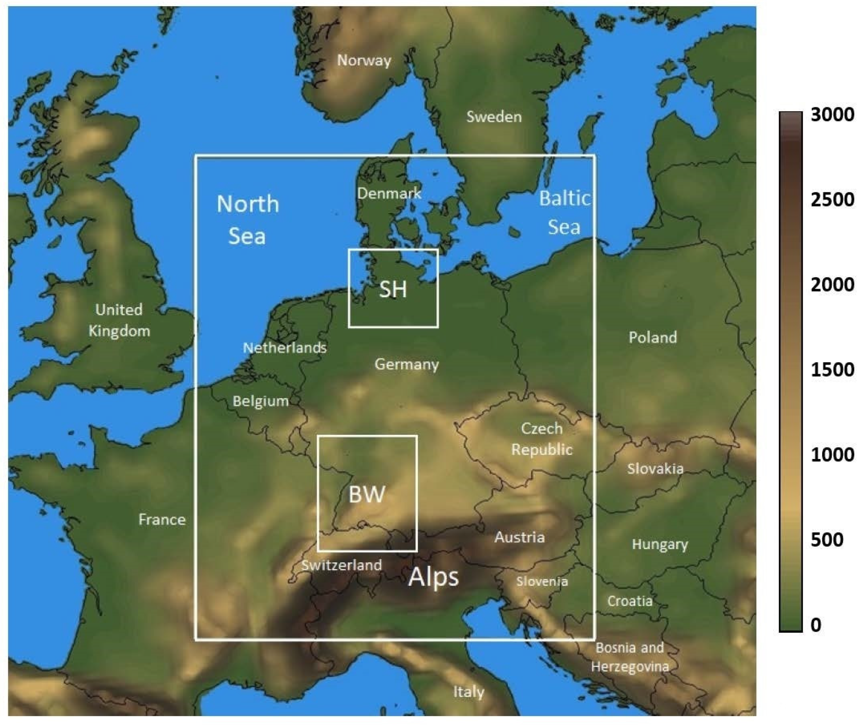
2.1. Model Setup and Study Areas

The Weather Research and Forecasting model version 4 (Forecasting (WRF v4.0 ARW, https://www2.mmm.ucar.edu/wrf/users/download/get_source.html, accessed on 16 July 2022, hereafter WRF) [36,37,38], a next-generation mesoscale numerical weather prediction system, is used to simulate the precipitation events. The model is configured in a nesting approach. The parent domain consists of 120 × 150 grid cells in the west–east and south–north directions, respectively, with a 9 km cell resolution, centered at (51° N, 9.8° E) stretching into the sea to the north and including the Alps to the south, to accommodate weather systems influenced by synoptic-scale circulations that originate overseas or are affected by the complex topography of the Alpine region (Figure 1).
Both nested domains have a grid resolution of 3 km. The northern Schleswig–Holstein (SH) domain consists of 79 × 79 grid cells, while the lower Baden–Wurttemberg (BW) domain has 82 × 112 grid cells in the west–east and south–north direction. In the vertical direction, the model used 40 layers. The ERA5 atmospheric reanalysis at 0.25° spatial resolution is used as the forcing dataset for the single initial and lateral boundary conditions of the parent domain [60,61] feeding the model every 6 h. A spin-up time of 24 h has been used in all experiments. The study areas chosen were SH and BW. The SH region is located in the northern part of Germany, affected by systems coming from the North Sea and the Baltic Sea and presenting smooth topography. It is one of the coldest regions in Germany with a mean annual temperature of 9 °C and a mean monthly precipitation of 39.9 mm (478.4 mm per year). It has a humid climate with a mean relative humidity of 80% and receives rainfall all months on an annual basis. The BW region is located in the southwestern part of Germany, in proximity to the Alps, presenting complex topography and a mean temperature of 11 °C and mean monthly precipitation of 28.8 mm (345.1 mm per year). It is less humid than SH with a mean relative humidity of 75%.

2.2. Observational Data and Event Selection

The precipitation events chosen for the sensitivity analysis performed herein were selected from the catalogue of spatially and temporally independent heavy precipitation events provided by the German Weather Service (DWD) (Table 1, available at https://cdc.dwd.de/portal/ accessed on 17 December 2022). The methodology for deriving extreme precipitation events was based on radar precipitation estimates on a 1 km × 1 km grid over Germany resulting from hourly sums and adjusted to station data. Precipitation objects, i.e., regions of adjacent grids receiving precipitation over a specific value, for a specific time frame, which exceeded DWD’s warning level 3, i.e., rainfall more than 40 mm/h, for severe weather (W3) [62] were identified. For each region, two near-summer and two near-winter events were chosen so that model performance could be validated thoroughly. The selection was primarily based on the affected area, so that an adequate number of meteorological stations was included, and the extremity (Eta), a parameter dependent on the return period and the affected area of an event, as proposed by Müller and Kaspar [63].

2.3. Physics Parameterizations

Precipitation, as a process within the WRF model, is mainly driven by three key schemes: microphysics (MP), cumulus (CU) and planetary boundary layer (PBL). Therefore, these are examined in this study in search for an optimal configuration that can generate a reliable precipitation simulation of the selected events.
The MP scheme provides atmospheric heat and moisture tendencies, microphysical rates, and determines the actions of the water particles, and is therefore responsible for cloud formation. It also governs surface rainfall and designates surface–atmosphere interactions. The MP parameterizations examined were the Kessler scheme (KS), the Eta (Ferrier) scheme (ES), the WRF Single–Moment 6–Class scheme (WSM6), the Single–Moment 5–Class scheme (WSM5), and the Morrison 2-Moment scheme (MDM). Rain originating from non-ice-phase activities in clouds (warm rain), formed principally by coalescence of water droplets of various sizes as they descend at varied terminal velocities inside the clouds, is the main feature of the KS Single Moment scheme [64]. In marine clouds, warm rain mechanisms are most common. It does not generate ice, hail, graupel, or snow. The ES scheme [65] uses advection of total condensate. Cloud water, rain, and ice (cloud ice, snow/graupel) come from storage arrays, and it assumes fixed fractions of water and ice within the column during advection. It considers suspended cloud liquid water droplets, rain, large ice (snow, graupel, sleet, etc.) and small ice (suspended cloud ice) as hydrometeors. The WSM5 scheme [56] includes ice, no graupel or hail. It also incorporates supercooled water, snow melt and ice sedimentation. Using the Bergeron process, it presents a realistic mixed phase, initializing precipitation in a mixed cloud with a temperature below freezing. Finally, the WSM6 scheme [44] incorporates the processes of water vapor, cloud water, cloud ice, snow, rain, and graupel. The Morrison 2-Moment scheme [50] is a 6-class microphysics scheme with graupel. It predicts number concentrations also for ice, snow, rain, and graupel.
The CU scheme produces clouds for the microphysics, it provides atmospheric heat and moisture/cloud tendency profiles, and it establishes the convective fluxes and handles surface subgrid-scale convective rainfall. It also provides the cloud fraction for the radiation. In our study, we examined the Kain–Fritsch scheme (KF), Betts–Miller–Janjic scheme (BMJ), and Grell–Freitas Ensemble scheme (GF). The KF [49] is a mass flux parameterization scheme, determining updraft and downdraft fluxes. It estimates if instability occurs, whether any current instability will become accessible for cloud development, and what the attributes of any convective clouds could be, using the Lagrangian parcel approach with vertical momentum dynamics. The BMJ [45] is not a mass flux scheme but an adjustment-type scheme; convective processes are worked out from the profiles of the reference temperature and moisture, which are created based on a large number of observations. The GF scheme [46] has a working mechanism that uses a probability density function in combination with a data assimilation technique.
The PBL scheme distributes boundary layer fluxes of heat, moisture, and momentum, along with the vertical diffusion in the whole column. There are two classes of PBL schemes: local closure schemes, also known as turbulent kinetic energy (TKE) prediction schemes because they determine eddy diffusion coefficients from prognostic TKE, and the diagnostic nonlocal closure ones. Our study examines the Mellor–Yamada–Janjic (MYJ) and the Yonsei University (YSU) schemes, one from each class. The MYJ local closure scheme [45] solves for turbulent kinetic energy in each column, estimating buoyancy and wind shear, dissipation, and vertical mixing. Turbulent fluxes at each grid point are determined by the mean values of atmospheric variables and/or their gradients at that point. The YSU scheme [51], is a nonlocal scheme that diagnoses a PBL top, specifies a K profile [66], and expresses turbulent diffusion by adding a nonlocal gradient correction term.
Combining the abovementioned parameterization options, 30 different scenarios were created for the sensitivity analysis, presented in Table 2, for each of the eight events, leading to 240 simulations in total.

2.4. Performance Metrics

The statistical analysis carried out here employs 5 pairwise statistical measures and 6 categorical ones, presented in Table 3, namely Mean Absolute Error (MAE), Root Mean Square Error (RMSE), Index of Agreement (IoA), Covariance (COV), Pearson Correlation Coefficient (PCC), Probability of Detection (POD), False Alarm Ratio (FAR), Critical Success Index (CSI), Frequency Bias Index (FBI), Percent Correct (PC), and the Bias Adjusted Equitable Threat Score (BAETS) [67]. The statistical analysis is based on the hourly values for each model grid cell that contains a station in the examined domains. In Table 3, Xp and Xo denote the hourly gridded predicted and observed values, with n being the total number of grid points, while overbars denote mean values, H stands for the correct detections, Ζ stands for the false alarms, Y stands for the misses, W denotes the correct negatives, N denotes the total forecasts, O denotes the observed area (sum of correct detections, H, and misses, Y), and F stands for the forecast event (sum of correct detections, H, and false alarms, Z).
Each scenario is characterized by eleven mean regional statistical values. To conclude to the best performing parameterization combinations, the TOPSIS multicriteria decision-making method is employed. TOPSIS uses as input the eleven statistical metrics mentioned above for each scenario and ranks the options based on their distances from the ideal and negative ideal solutions, with the top option having the shortest distance from the positive ideal solution and the longest distance from the negative ideal solution.

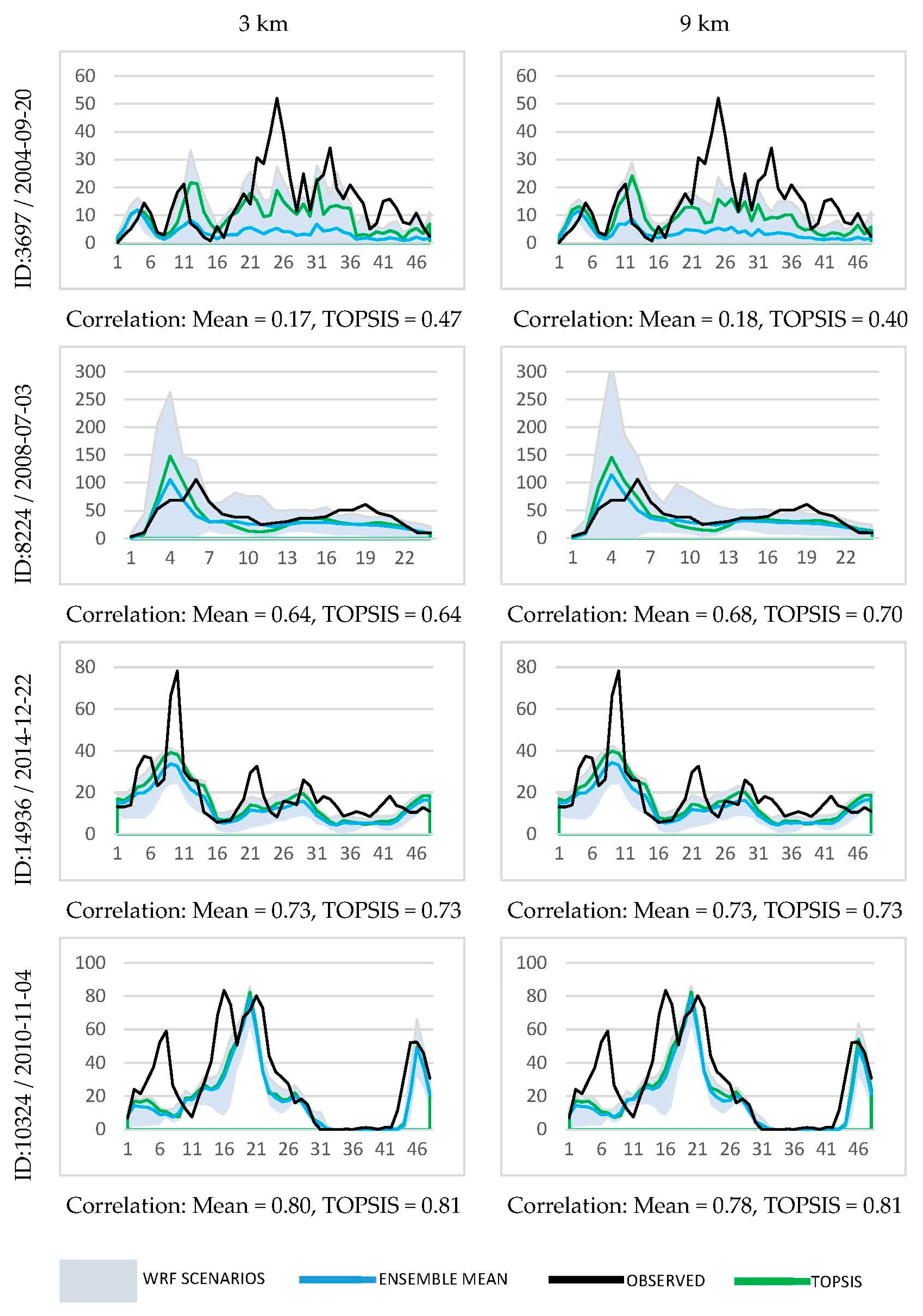
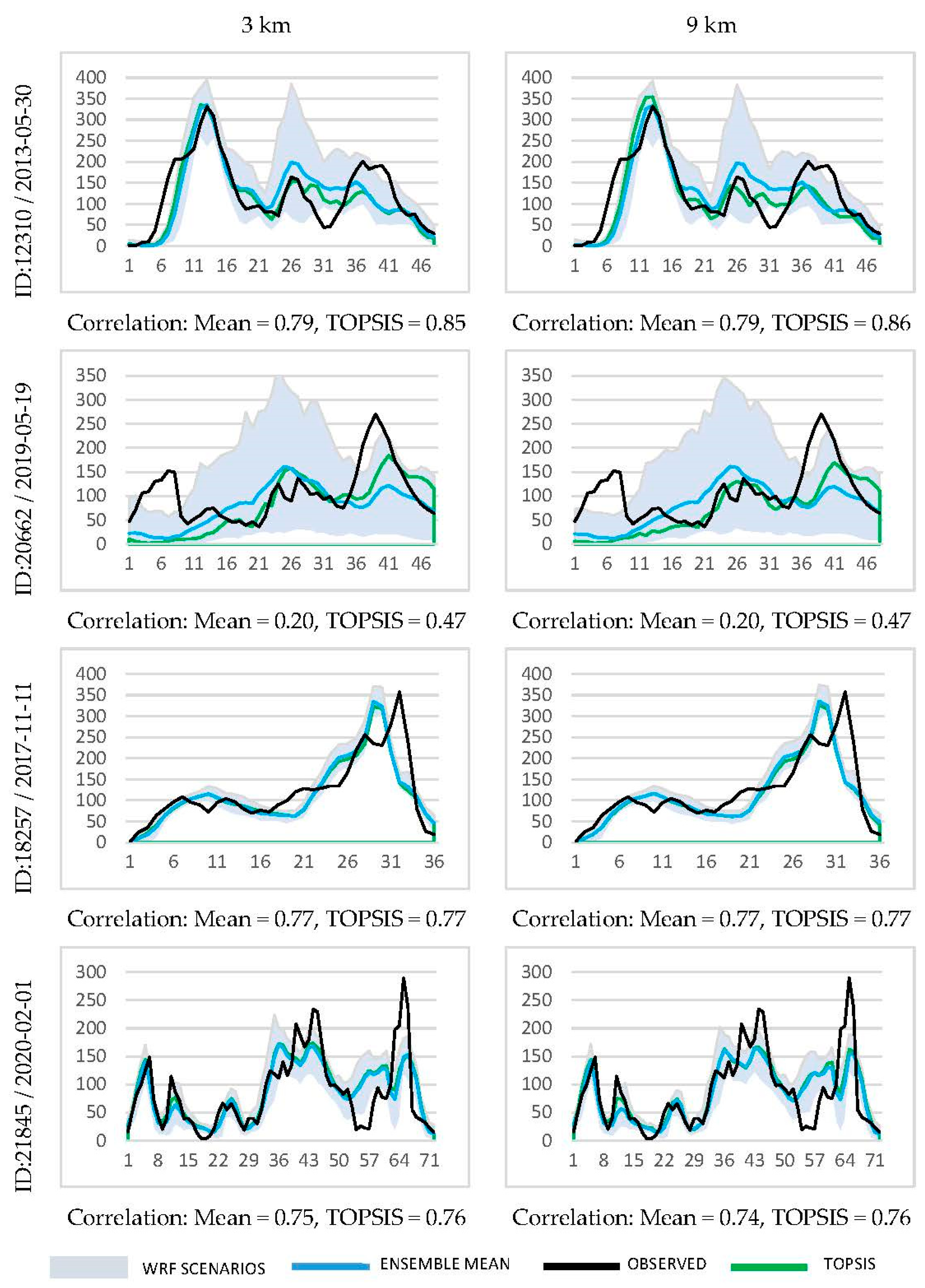
3. Results and Discussion

WRF Temporal Performance

Table 4 presents the results of the TOPSIS algorithm for each of the eight rainfall episodes under study. Apparently, in almost all episodes, the best scenario for the 3 and 9 km simulations is common, together with the fact that in the list of the top 5 performing scenarios the combinations found are almost the same.
In Table 5, the ranking summary for each parameterization as a percentage for appearing in the five best performing scenarios according to TOPSIS is presented. Most of the single top-ranking scenarios employed the MDM MP scheme followed by the WSM6, the GF CU scheme, and the YSU PBL scheme. As an overall performance for both resolutions and all events, the MDM MP scheme appears in 30% of the top five scenarios followed by the WSM5 with a 27.5% occurrence. The differences between percentages are not that large, which is evident of an adequate performance for nearly all the MP schemes, apart from the model’s default KS. Looking at the CU schemes, GF and KF appear in the highest percentage of top-performing combinations, while the BMJ shows in just a few cases. Finally, for the PBL schemes, the YSU encounters more frequently (57.50%) in the top five performance combinations compared to the MYJ scheme.
In the next step, the data for all precipitation events were fed into the TOPSIS algorithm to identify which parameterization combination would rank as the best if it treated all events as one. For the 3 km simulation the MDM–GF–YSU and for the 9 km the MDM–GF–MYJ were ranked first (Table 6), similar to that reported by Umer et al. [53]. Additionally, along the lines of the reasoning above, the TOPSIS algorithm was fed with all the episodes that were near-summer and then those that were near-winter. Near-summer events are better simulated by the MDM–GF–MYJ combination and the MDM–KF–YSU for the 3 and 9 km resolutions, respectively, while near-winter events are better simulated by the WSM5–KF–YSU and the WSM6–GF–YSU combinations (for 3 and 9 km, respectively). Then, the algorithm was fed with all the data from the episodes that occurred in the north and afterward those in the south. The top setup for the northern SH region is EF–GF–YSU for both resolutions while for the southern BW region the MDM–GF–MYJ and the EF–KF–MYJ (3 km/9 km). The region and season specific ranking results are presented in Table 6.
It must be stated that any parameterization scheme is not as crucial on its own but as part of a combination in delivering a result. Surely, the presence of a given scheme in combinations generating minor variations from observed values indicates dependable scheme performance. However, the various combinations must be considered as distinct choices and their performances validated. The MDM–GF–YSU, WSM5–KF–YSU, and the WSM5–GF–YSU are the three more frequent combinations encountered in the top five TOPSIS performance ranks when assessing all events individually for both 3 and 9 km grid cell distances.
Figure 2 and Figure 3 present the temporal hourly evolution of the recorded area-averaged precipitation for each distinct event (black line) and both grid size resolutions (i.e., 3 and 9 km). The light blue line depicts the average precipitation derived from all the different model setups that were examined in this study. The green line indicates the average hourly area precipitation derived from the five best-performing model configurations according to the TOPSIS algorithm ranking. Finally, the gray area represents the dispersion of average precipitation values from the various setups that were used to perform the simulations. Figure 2 shows the four extreme rainfall events that occurred over the SH region located in the north, while Figure 3 presents the four events for the southern region of BW. In each case, the correlation values between the model average and the recorded rainfall data (correlation mean) are presented, together with the correlation between the average of the five best-performing setups and the recorded data (correlation TOPSIS).
Regarding the SH area near-summer event (ID:3697), the model performed poorly, with the mean values from all parameterizations differing substantially from the observed ones, leading to a low correlation value of 0.17 for the mean model performance for the 3 km simulations and 0.18 for the ones conducted at the 9 km resolution. After applying the TOPSIS algorithm, the mean precipitation value for the five best scenarios was estimated, increasing the correlations to 0.47 and 0.40 for the 3 and 9 km resolutions, respectively (Figure 2, first row).
The improvement is significant as far as the temporal variation is concerned, but the peak amount of precipitation was still not predicted adequately by the model. For the other near-summer event (ID:8224), the model ensemble mean-estimated peak precipitation value is similar to the actual one, and after the application of the TOPSIS algorithm it is slightly overestimated by the mean of the top five ranking parameterization combinations (Figure 2, second row). The model failed to estimate the peak rainfall hour, predicting it earlier than the observed one. For the 3 km simulations, the TOPSIS technique did not add any value to the results since the average model performance from all parameterization combinations had a similar correlation value. For the 9 km simulations, results are similar, with a small correlation improvement after the application of TOPSIS, from 0.68 to 0.70. Temporarily, the predicted peak hour is again a few hours earlier than the recorded. Near-winter events (IDs 10324, 14936) present high correlation values for mean model performance, and the model accurately predicted the peak hour. In both winter events, the dispersion of model values is low as it is obvious from the narrow gray areas in Figure 2, rows 3 and 4. The model underestimated the peak amount of precipitation for the ID:14936 event, while it successfully predicted the peak hour. The application of the TOPSIS algorithm did not improve correlation but, as it is obvious from Figure 2 (third row), it narrowed the difference between the predicted and the recorded peak rainfall amount in both the 3 and 9 km simulations. For the ID:10324 event, applying the TOPSIS algorithm slightly improved correlation values since all model scenarios had a relatively similar performance. The model failed to depict the rainfall amount at the beginning of the episode, while it predicted the peak rainfall amount but not the overall duration of the heavy rainfall.
In the BW area, near-summer events (IDs 12310, 20662) are better simulated by the model, especially after application of the TOPSIS algorithm, for which correlation values improve significantly. It is also evident that the model’s different parameterization scenarios exhibit a notable high dispersion, as it was for the warm-season case in the SH area. For the ID:12310 event, the model succeeds in predicting the peak hour as well as the maximum amount of precipitation. The TOPSIS algorithm improves correlation for both the 3 and 9 km simulations, from 0.79 to 0.85 and 0.86, respectively. The TOPSIS mean reduces the difference between the recorded values at the second small increase in rainfall around hour 26. For the ID:20662 event, the model correctly estimated the peak hour but not the peak amount of rainfall. It failed in depicting the increased early rainfall amount, but afterward it performed relatively well. The TOPSIS algorithm added significant value, improving correlation from 0.20 to 0.47 for the 3 and 9 km simulations. Near-winter event simulations (IDs 18257, 21845), exhibit small dispersion in model output and the TOPSIS algorithm adds little value to the model performance. For the ID:18257 event, the model predicted the peak hour a little earlier and succeeded in predicting the peak precipitation amount. The 3 and 9 km simulation results are similar with all parameterization scenarios exhibiting adequate performance; thus, the TOPSIS technique does not improve model correlation. On the other hand, for the ID:21845 event, the model was more accurate in predicting the peak hour but not the maximum amount of precipitation. In this case, the TOPSIS algorithm slightly improved model performance.
It is also evident from Figure 2 and Figure 3 (first two rows) that during the near-summer events, many of the parameterization combinations examined fail to predict the evolution of precipitation, leading to a wide gray area representing the dispersion of rainfall amount values for the various setups. This may be attributed to the nature of summer precipitation, where the heating of the underlying air layers is much faster than in winter, leading to their rapid rise in the atmosphere and ultimately the precipitation generation. In contrast to summer, all combinations of parameterizations predict the evolution of precipitation events quite well (Figure 2 and Figure 3, rows 3 and 4), since the corresponding mechanism acts much more slowly in an atmosphere where more stable conditions prevail.

4. Conclusions

The performance of the WRF model is assessed by means of a wide set of microphysics, cumulus, and planetary boundary layer scheme combinations for a total of eight extreme precipitation events that occurred in the regions of SH and BW in Germany. The primary reason for choosing these specific research sites is related to the distinct climate and weather systems that govern these regions. The model is tested separately for the near-summer and near-winter seasons. The initial and lateral boundary conditions are provided by the ERA5 reanalysis dataset. Simulation results are compared against observational station data obtained from the German weather service DWD.
The findings of this study suggest that increasing the spatial resolution of the model from 9 to 3 km grid cell size had very little impact on the performance of the model. As a result, fine resolution could be disregarded, boosting the computational efficiency of the forecast. The combination that produced the best results was the same regardless of the spatial resolution that was employed, except for a few specific cases. When looking at the rainfall events that occurred during the summer months, the outputs of the various model configurations showed large discrepancies. On the other hand, the dispersion of the findings became substantially less noticeable during the winter months.
Looking at the different events as separate from one another and the frequency of occurrence of the various schemes in the top-ranking combinations, it was revealed that the MDM MP scheme appeared in the majority of them, followed by WSM6. In terms of the CU scheme, the GF is the dominant parameterization in the top performing combination members, whereas the YSU outperforms in the PBL scheme. It should be mentioned here that when looking at the top five ranking results, the dominance of these observed schemes lessens because the majority of the schemes were part of a combination that had adequate simulation performance.
Feeding all statistical measures from all precipitation events into the TOPSIS algorithm, essentially assuming that all events under consideration were a single event, it was found that the top parameterization combinations are the MDM–GF–MYJ and MDM–GF–YSU for the 3 and 9 km spatial resolutions, respectively. Similarly, when all the events near-summer and the corresponding ones near-winter were fed into the TOPSIS algorithm, the combinations with the best performance for the events near-summer were MDM–GF–MYJ and MDM–KF–YSU for the 3 and 9 km grid spacing, respectively, while the top-ranking combos for the ones near-winter were WSM5–KF–YSU and WSM6–GF–YSU. Finally, depending on the geographical location, the optimal combinations were investigated, yielding EF–GF–YSU for the northern region for both grid cell distances and WSM5–GF–MYJ/EF–GF–YSU for the southern region for 3 km/9 km simulations.
Identifying the most appropriate combination of model physics parameterizations along with a representative grid size resolution is undeniably important in precipitation forecast attempts. Here, taking into account the small added value of increasing the model’s resolution on the optimization of the results and the need to choose an ensemble that will be able to produce accurate results in any case, we propose the MDM–GF–YSU (MP–CU–PBL schemes) ensemble for forecasting heavy rainfall events in the region of Germany at a grid spacing of 9 km.

Author Contributions

Conceptualization, I.S., E.T. and R.-E.P.S.; methodology, I.S., E.T. and R.-E.P.S.; software, I.S.; validation, I.S.; formal analysis, E.T. and R.-E.P.S.; investigation, I.S., E.T. and R.-E.P.S.; resources, E.T. and R.-E.P.S.; data curation, I.S.; writing—original draft preparation, I.S.; writing—review and editing, E.T. and R.-E.P.S.; visualization, I.S.; supervision, R.-E.P.S.; project administration, R.-E.P.S. All authors have read and agreed to the published version of the manuscript.

Funding

This work was supported by the Project “Development of New Innovative Low Carbon Foot-print Energy Technologies to Enhance Excellence in the Region of Western Macedonia” (MIS 5047197), which is implemented under the Action “Reinforcement of the Research and Innovation Infrastructure”, funded by the Operational Programme “Competitiveness, Entrepreneurship and Innovation” (NSRF 2014–2020), and co-financed by Greece and the European Union (European Regional Development Fund).

Institutional Review Board Statement

Not applicable.

Informed Consent Statement

Not applicable.

Data Availability Statement

Not applicable.

Conflicts of Interest

The authors declare no conflict of interest.

References

  1. Masson-Delmotte, V.; Zhai, P.; Pirani, A.; Connors, S.L.; Péan, C.; Berger, S.; Caud, N.; Chen, Y.; Goldfarb, L.; Gomis, M.I. (Eds.) IPCC Climate Change 2021: The Physical Science Basis. Contribution of Working Group I to the Sixth Assessment Report of the Intergovernmental Panel on Climate Change; Cambridge University Press: Cambridge, UK, 2021; in press. [Google Scholar]
  2. Trnka, M.; Vizina, A.; Hanel, M.; Balek, J.; Fischer, M.; Hlavinka, P.; Semerádová, D.; Štěpánek, P.; Zahradníček, P.; Skalák, P.; et al. Increasing Available Water Capacity as a Factor for Increasing Drought Resilience or Potential Conflict over Water Resources under Present and Future Climate Conditions. Agric. Water Manag. 2022, 264, 107460. [Google Scholar] [CrossRef]
  3. Chiang, F.; Mazdiyasni, O.; AghaKouchak, A. Evidence of Anthropogenic Impacts on Global Drought Frequency, Duration, and Intensity. Nat. Commun. 2021, 12, 2754. [Google Scholar] [CrossRef] [PubMed]
  4. Afshar, M.H.; Şorman, A.Ü.; Tosunoğlu, F.; Bulut, B.; Yilmaz, M.T.; Danandeh Mehr, A. Climate Change Impact Assessment on Mild and Extreme Drought Events Using Copulas over Ankara, Turkey. Theor. Appl. Climatol. 2020, 141, 1045–1055. [Google Scholar] [CrossRef]
  5. Spinoni, J.; Barbosa, P.; Bucchignani, E.; Cassano, J.; Cavazos, T.; Christensen, J.H.; Christensen, O.B.; Coppola, E.; Evans, J.; Geyer, B.; et al. Future Global Meteorological Drought Hot Spots: A Study Based on CORDEX Data. J. Clim. 2020, 33, 3635–3661. [Google Scholar] [CrossRef]
  6. Trenberth, K.E.; Dai, A.; Rasmussen, R.M.; Parsons, D.B. The Changing Character of Precipitation. Bull. Am. Meteorol. Soc. 2003, 84, 1205–1218. [Google Scholar] [CrossRef]
  7. Berg, P.; Christensen, O.B.; Klehmet, K.; Lenderink, G.; Olsson, J.; Teichmann, C.; Yang, W. Summertime Precipitation Extremes in a EURO-CORDEX 0.11° Ensemble at an Hourly Resolution. Nat. Hazards Earth Syst. Sci. 2019, 19, 957–971. [Google Scholar] [CrossRef] [Green Version]
  8. Prein, A.F.; Rasmussen, R.M.; Ikeda, K.; Liu, C.; Clark, M.P.; Holland, G.J. The Future Intensification of Hourly Precipitation Extremes. Nat. Clim. Chang. 2017, 7, 48–52. [Google Scholar] [CrossRef]
  9. Kharin, V.V.; Zwiers, F.W.; Zhang, X.; Hegerl, G.C. Changes in Temperature and Precipitation Extremes in the IPCC Ensemble of Global Coupled Model Simulations. J. Clim. 2007, 20, 1419–1444. [Google Scholar] [CrossRef] [Green Version]
  10. Ali, H.; Mishra, V. Increase in Subdaily Precipitation Extremes in India Under 1.5 and 2.0 °C Warming Worlds. Geophys. Res. Lett. 2018, 45, 6972–6982. [Google Scholar] [CrossRef] [Green Version]
  11. Papalexiou, S.M.; Montanari, A. Global and Regional Increase of Precipitation Extremes Under Global Warming. Water Resour. Res. 2019, 55, 4901–4914. [Google Scholar] [CrossRef]
  12. Zhang, W.; Zhou, T. Significant Increases in Extreme Precipitation and the Associations with Global Warming over the Global Land Monsoon Regions. J. Clim. 2019, 32, 8465–8488. [Google Scholar] [CrossRef]
  13. Ju, J.; Wu, C.; Yeh, P.J.-F.; Dai, H.; Hu, B.X. Global Precipitation-Related Extremes at 1.5 °C and 2 °C of Global Warming Targets: Projection and Uncertainty Assessment Based on the CESM-LWR Experiment. Atmos. Res. 2021, 264, 105868. [Google Scholar] [CrossRef]
  14. Li, X.; Zhang, K.; Gu, P.; Feng, H.; Yin, Y.; Chen, W.; Cheng, B. Changes in Precipitation Extremes in the Yangtze River Basin during 1960–2019 and the Association with Global Warming, ENSO, and Local Effects. Sci. Total Environ. 2021, 760, 144244. [Google Scholar] [CrossRef] [PubMed]
  15. Franzke, C.L.E. Changing Temporal Volatility of Precipitation Extremes Due to Global Warming. Int. J. Climatol. 2022, 1–13. [Google Scholar] [CrossRef]
  16. Chinita, M.J.; Richardson, M.; Teixeira, J.; Miranda, P.M.A. Global Mean Frequency Increases of Daily and Sub-Daily Heavy Precipitation in ERA5. Environ. Res. Lett. 2021, 16, 074035. [Google Scholar] [CrossRef]
  17. Argüeso, D.; Hidalgo-Muñoz, J.M.; Gámiz-Fortis, S.R.; Esteban-Parra, M.J.; Dudhia, J.; Castro-Díez, Y. Evaluation of WRF Parameterizations for Climate Studies over Southern Spain Using a Multistep Regionalization. J. Clim. 2011, 24, 5633–5651. [Google Scholar] [CrossRef]
  18. Kan, Y.; Liu, C.; Liu, Y.; Zhou, C. Evaluation of WRF Microphysics and Cumulus Parameterization Schemes in Simulating a Heavy Rainfall Event over Yangtze River Delta. In Proceedings of the Remote Sensing and Modeling of Ecosystems for Sustainability XII, 96100R, San Diego, CA, USA, 4 September 2015; Gao, W., Chang, N.-B., Wang, J., Eds.; SPIE: Bellingham, DC, USA, 2015. [Google Scholar]
  19. Rezazadeh, M.; Moradian, F.; Ghader, S. Evaluation of a WRF Model Multi-Physics Ensemble Forecasting System for Simulation of Precipitation over Central Region of Iran. Iran. J. Geophys. 2020, 14, 13–38. [Google Scholar] [CrossRef]
  20. Douluri, D.L.; Chakraborty, A. Assessment of WRF-ARW Model Parameterization Schemes for Extreme Heavy Precipitation Events Associated with Atmospheric Rivers over West Coast of India. Atmos. Res. 2021, 249, 105330. [Google Scholar] [CrossRef]
  21. Liu, H.; Zhao, X.; Duan, K.; Shang, W.; Li, M.; Shi, P. Optimizing Simulation of Summer Precipitation by Weather Research and Forecasting Model over the Mountainous Southern Tibetan Plateau. Atmos. Res. 2023, 281, 106484. [Google Scholar] [CrossRef]
  22. Prein, A.F.; Langhans, W.; Fosser, G.; Ferrone, A.; Ban, N.; Goergen, K.; Keller, M.; Tölle, M.; Gutjahr, O.; Feser, F.; et al. A Review on Regional Convection-Permitting Climate Modeling: Demonstrations, Prospects, and Challenges. Rev. Geophys. 2015, 53, 323–361. [Google Scholar] [CrossRef]
  23. Conil, S.; Hall, A. Local Regimes of Atmospheric Variability: A Case Study of Southern California. J. Clim. 2006, 19, 4308–4325. [Google Scholar] [CrossRef]
  24. Pielke, R.A., Sr.; Beltrán-Przekurat, A.; Hiemstra, C.A.; Lin, J.; Nobis, T.E.; Adegoke, J.; Nair, U.S.; Niyogi, D. Impacts of Regional Land Use and Land Cover on Rainfall: An Overview. In Climate Variability and Change—Hydrological Impacts; Demuth, S., Gustard, A., Planos, E., Scatena, F., Servat, E., Eds.; IAHS Press: Oxford, UK, 2006; Volume 308, pp. 325–331. [Google Scholar]
  25. Cao, Q.; Yu, D.; Georgescu, M.; Han, Z.; Wu, J. Impacts of Land Use and Land Cover Change on Regional Climate: A Case Study in the Agro-Pastoral Transitional Zone of China. Environ. Res. Lett. 2015, 10, 124025. [Google Scholar] [CrossRef]
  26. Kirthiga, S.M.; Patel, N.R. Impact of Updating Land Surface Data on Micrometeorological Weather Simulations from the WRF Model. Atmósfera 2018, 31, 165–183. [Google Scholar] [CrossRef] [Green Version]
  27. Madala, S.; Salinas, S.V.; Wang, J.; Liew, S.C. Customization of the Advanced Research Weather Research and Forecasting Model over the Singapore Region: Impact of Planetary Boundary Layer Schemes, Land Use, Land Cover and Model Horizontal Grid Resolution. Meteorol. Appl. 2019, 26, 221–231. [Google Scholar] [CrossRef] [Green Version]
  28. Zhao, D.; Wu, J. Evaluating Land Use Change Impacts on Rainfall in Various Categories Using the Weather Research and Forecasting-Mosaic Approach. Atmos. Sci. Lett. 2019, 20, e870. [Google Scholar] [CrossRef] [Green Version]
  29. Zan, B.; Yu, Y.; Dong, L.; Li, J.; Zhao, G.; Zhang, T. Numerical Study of the Impact of Complex Terrain and Soil Moisture on Convective Initiation. Atmosphere 2020, 11, 871. [Google Scholar] [CrossRef]
  30. Golzio, A.; Ferrarese, S.; Cassardo, C.; Diolaiuti, G.A.; Pelfini, M. Land-Use Improvements in the Weather Research and Forecasting Model over Complex Mountainous Terrain and Comparison of Different Grid Sizes. Bound.-Layer Meteorol. 2021, 180, 319–351. [Google Scholar] [CrossRef]
  31. Fosser, G.; Khodayar, S.; Berg, P. Benefit of Convection Permitting Climate Model Simulations in the Representation of Convective Precipitation. Clim. Dyn. 2014, 44, 45–60. [Google Scholar] [CrossRef] [Green Version]
  32. Cassola, F.; Ferrari, F.; Mazzino, A. Numerical Simulations of Mediterranean Heavy Precipitation Events with the WRF Model: A Verification Exercise Using Different Approaches. Atmos. Res. 2015, 164–165, 210–225. [Google Scholar] [CrossRef]
  33. Zittis, G.; Bruggeman, A.; Camera, C.; Hadjinicolaou, P.; Lelieveld, J. The Added Value of Convection Permitting Simulations of Extreme Precipitation Events over the Eastern Mediterranean. Atmos. Res. 2017, 191, 20–33. [Google Scholar] [CrossRef]
  34. Van de Walle, J.; Thiery, W.; Brousse, O.; Souverijns, N.; Demuzere, M.; van Lipzig, N.P.M. A Convection-Permitting Model for the Lake Victoria Basin: Evaluation and Insight into the Mesoscale versus Synoptic Atmospheric Dynamics. Clim. Dyn. 2020, 54, 1779–1799. [Google Scholar] [CrossRef]
  35. Hodnebrog, Ø.; Steensen, B.M.; Marelle, L.; Alterskjær, K.; Dalsøren, S.B.; Myhre, G. Understanding Model Diversity in Future Precipitation Projections for South America. Clim. Dyn. 2022, 58, 1329–1347. [Google Scholar] [CrossRef]
  36. Skamarock, W.C.; Klemp, J.B.; Dudhia, J.; Gill, D.O.; Liu, Z.; Berner, J.; Wang, W.; Powers, J.G.; Duda, M.G.; Barker, D.M.; et al. A Description of the Advanced Research WRF Model Version 4; UCAR/NCAR; National Center for Atmospheric Research: Boulder, CO, USA, 2019. [Google Scholar]
  37. Powers, J.G.; Klemp, J.B.; Skamarock, W.C.; Davis, C.A.; Dudhia, J.; Gill, D.O.; Coen, J.L.; Gochis, D.J.; Ahmadov, R.; Peckham, S.E.; et al. The Weather Research and Forecasting Model: Overview, System Efforts, and Future Directions. Bull. Amer. Meteor. Soc. 2017, 98, 1717–1737. [Google Scholar] [CrossRef]
  38. Skamarock, C.; Klemp, B.; Dudhia, J.; Gill, O.; Barker, D.; Duda, G.; Huang, X.; Wang, W.; Powers, G. A Description of the Advanced Research WRF Version 3; Citeseer: University Park, PA, USA, 2008. [Google Scholar] [CrossRef]
  39. Hwang, C.-L.; Yoon, K. Methods for Multiple Attribute Decision Making. In Multiple Attribute Decision Making: Methods and Applications A State-of-the-Art Survey; Hwang, C.-L., Yoon, K., Eds.; Lecture Notes in Economics and Mathematical Systems; Springer: Berlin/Heidelberg, Germany, 1981; pp. 58–191. ISBN 978-3-642-48318-9. [Google Scholar]
  40. Yoon, K. A Reconciliation among Discrete Compromise Solutions. J. Oper. Res. Soc. 1987, 38, 277–286. [Google Scholar] [CrossRef]
  41. Hwang, C.-L.; Lai, Y.-J.; Liu, T.-Y. A New Approach for Multiple Objective Decision Making. Comput. Oper. Res. 1993, 20, 889–899. [Google Scholar] [CrossRef]
  42. Duzenli, E.; Yucel, I.; Pilatin, H.; Yilmaz, M.T. Evaluating the Performance of a WRF Initial and Physics Ensemble over Eastern Black Sea and Mediterranean Regions in Turkey. Atmos. Res. 2021, 248, 105184. [Google Scholar] [CrossRef]
  43. Liu, Y.; Chen, Y.; Chen, O.; Wang, J.; Zhuo, L.; Rico-Ramirez, M.A.; Han, D. To Develop a Progressive Multimetric Configuration Optimisation Method for WRF Simulations of Extreme Rainfall Events over Egypt. J. Hydrol. 2021, 598, 126237. [Google Scholar] [CrossRef]
  44. Hong, S.Y.; Lim, J.-O.J. The WRF Single-Moment 6-Class Microphysics Scheme (WSM6). Asia-Pac. J. Atmos. Sci. 2006, 42, 129–151. [Google Scholar]
  45. Janjić, Z.I. The Step-Mountain Eta Coordinate Model: Further Developments of the Convection, Viscous Sublayer, and Turbulence Closure Schemes. Mon. Weather. Rev. 1994, 122, 927–945. [Google Scholar] [CrossRef]
  46. Grell, G.A.; Freitas, S.R. A Scale and Aerosol Aware Stochastic Convective Parameterization for Weather and Air Quality Modeling. Atmos. Chem. Phys. 2014, 14, 5233–5250. [Google Scholar] [CrossRef]
  47. Freitas, S.R.; Grell, G.A.; Molod, A.; Thompson, M.A.; Putman, W.M.; Santos e Silva, C.M.; Souza, E.P. Assessing the Grell-Freitas Convection Parameterization in the NASA GEOS Modeling System. J. Adv. Modeling Earth Syst. 2018, 10, 1266–1289. [Google Scholar] [CrossRef] [PubMed]
  48. Wang, X.; Tolksdorf, V.; Otto, M.; Scherer, D. WRF-Based Dynamical Downscaling of ERA5 Reanalysis Data for High Mountain Asia: Towards a New Version of the High Asia Refined Analysis. Int. J. Climatol. 2021, 41, 743–762. [Google Scholar] [CrossRef]
  49. Kain, J.S. The Kain–Fritsch Convective Parameterization: An Update. J. Appl. Meteorol. Climatol. 2004, 43, 170–181. [Google Scholar] [CrossRef]
  50. Morrison, H.; Thompson, G.; Tatarskii, V. Impact of Cloud Microphysics on the Development of Trailing Stratiform Precipitation in a Simulated Squall Line: Comparison of One- and Two-Moment Schemes. Mon. Weather. Rev. 2009, 137, 991–1007. [Google Scholar] [CrossRef] [Green Version]
  51. Hong, S.-Y.; Noh, Y.; Dudhia, J. A New Vertical Diffusion Package with an Explicit Treatment of Entrainment Processes. Mon. Weather. Rev. 2006, 134, 2318–2341. [Google Scholar] [CrossRef] [Green Version]
  52. Niu, G.-Y.; Yang, Z.-L.; Mitchell, K.E.; Chen, F.; Ek, M.B.; Barlage, M.; Kumar, A.; Manning, K.; Niyogi, D.; Rosero, E.; et al. The Community Noah Land Surface Model with Multiparameterization Options (Noah-MP): 1. Model Description and Evaluation with Local-Scale Measurements. J. Geophys. Res. Atmos. 2011, 116, 15139. [Google Scholar] [CrossRef] [Green Version]
  53. Umer, Y.; Ettema, J.; Jetten, V.; Steeneveld, G.-J.; Ronda, R. Evaluation of the WRF Model to Simulate a High-Intensity Rainfall Event over Kampala, Uganda. Water 2021, 13, 873. [Google Scholar] [CrossRef]
  54. Pleim, J.E. A Combined Local and Nonlocal Closure Model for the Atmospheric Boundary Layer. Part I: Model Description and Testing. J. Appl. Meteorol. Climatol. 2007, 46, 1383–1395. [Google Scholar] [CrossRef]
  55. Bougeault, P.; Lacarrere, P. Parameterization of Orography-Induced Turbulence in a Mesobeta—Scale Model. Mon. Weather. Rev. 1989, 117, 1872–1890. [Google Scholar] [CrossRef]
  56. Hong, S.-Y.; Dudhia, J.; Chen, S.-H. A Revised Approach to Ice Microphysical Processes for the Bulk Parameterization of Clouds and Precipitation. Mon. Weather. Rev. 2004, 132, 103–120. [Google Scholar] [CrossRef]
  57. Sikder, S.; Hossain, F. Assessment of the Weather Research and Forecasting Model Generalized Parameterization Schemes for Advancement of Precipitation Forecasting in Monsoon-Driven River Basins. J. Adv. Modeling Earth Syst. 2016, 8, 1210–1228. [Google Scholar] [CrossRef] [Green Version]
  58. Thompson, G.; Field, P.R.; Rasmussen, R.M.; Hall, W.D. Explicit Forecasts of Winter Precipitation Using an Improved Bulk Microphysics Scheme. Part II: Implementation of a New Snow Parameterization. Mon. Weather. Rev. 2008, 136, 5095–5115. [Google Scholar] [CrossRef]
  59. Goodarzi, L.; Banihabib, M.E.; Roozbahani, A. A Decision-Making Model for Flood Warning System Based on Ensemble Forecasts. J. Hydrol. 2019, 573, 207–219. [Google Scholar] [CrossRef]
  60. Hersbach, H.; Bell, B.; Berrisford, P.; Hirahara, S.; Horányi, A.; Muñoz-Sabater, J.; Nicolas, J.; Peubey, C.; Radu, R.; Schepers, D.; et al. The ERA5 Global Reanalysis. Q. J. R. Meteorol. Soc. 2020, 146, 1999–2049. [Google Scholar] [CrossRef]
  61. Copernicus Climate Change Service (C3S) ERA5: Fifth Generation of ECMWF Atmospheric Reanalyses of the Global Climate. Copernicus Climate Change Service Climate Data Store (CDS). Available online: https://cds.climate.copernicus.eu/cdsapp#!/home (accessed on 8 November 2022).
  62. Lengfeld, K.; Walawender, E.; Winterrath, T.; Becker, A. CatRaRE: A Catalogue of Radar-Based Heavy Rainfall Events in Germany Derived from 20 Years of Data. Meteorol. Z. 2021, 30, 469–487. [Google Scholar] [CrossRef]
  63. Müller, M.; Kaspar, M. Event-Adjusted Evaluation of Weather and Climate Extremes. Nat. Hazards Earth Syst. Sci. 2014, 14, 473–483. [Google Scholar] [CrossRef] [Green Version]
  64. Kessler, E. On the Distribution and Continuity of Water Substance in Atmospheric Circulations. In On the Distribution and Continuity of Water Substance in Atmospheric Circulations; Kessler, E., Ed.; Meteorological Monographs; American Meteorological Society: Boston, MA, USA, 1969; pp. 1–84. ISBN 978-1-935704-36-2. [Google Scholar]
  65. Ferrier, B.S.; Jin, Y.; Lin, Y.; Black, T.; Rogers, E.; DiMego, G. Implementation of a New Grid-Scale Cloud and Precipitation Scheme in the NCEP Eta Model. In Proceedings of the 19th Conference on weather Analysis and Forecasting/15th Conference on Numerical Weather Prediction, San Antonio, TX, USA, 15 August 2002. [Google Scholar]
  66. Noh, Y.; Cheon, W.G.; Hong, S.Y.; Raasch, S. Improvement of the K-Profile Model for the Planetary Boundary Layer Based on Large Eddy Simulation Data. Bound.-Layer Meteorol. 2003, 107, 401–427. [Google Scholar] [CrossRef] [Green Version]
  67. Mesinger, F. Bias Adjusted Precipitation Threat Scores. Adv. Geosci. 2008, 16, 137–142. [Google Scholar] [CrossRef]
Figure 1. WRF model spatial configuration. The color bar depicts elevation (m).
Atmosphere 14 00017 g001
Figure 2. Hourly evolution of precipitation for the 3 and 9 km simulation results for the Schleswig–Holstein area. Black line—observed area-averaged precipitation for each distinct event; light blue line—average WRF-derived precipitation of all members; green line—average top-five-performing configurations according to TOPSIS; gray area—dispersion of average precipitation values from the various setups that were used to perform the simulations (vertical axis units are mm and horizontal axis units are h).
Atmosphere 14 00017 g002
Figure 3. Same as Figure 2 but for the Baden–Wurttemberg area.
Atmosphere 14 00017 g003
Table 1. Selected precipitation events.
RegionEvent IDStarting DateEnding DateDuration
(h)
Area
(km2)
Maximum Hourly Precipitation
(mm)
Mean Hourly Precipitation
(mm)
EtaNumber of Stations
Baden–Wurttemberg206622019-05-19
17:50:00
2019-05-21
17:50:00
483742180.57932108
123102013-05-30
18:49:59
2013-06-01
18:49:59
488743139.873.850.4108
218452020-02-01
10:50:00
2020-02-04
10:50:00
723258.4191.6118.443.7108
182572017-11-11
14:50:00
2017-11-12
14:50:00
364987.9141.969.840.5112
Schleswig–Holstein82242008-07-03
14:50:00
2008-07-04
14:50:00
2411,803.1137.76574.420
36972004-09-20
09:49:59
2004-09-22
09:49:59
484771.6120.768.533.113
149362014-12-22
01:50:00
2014-12-24
01:50:00
482261.888.469.5 22.615
103242010-11-04
02:50:00
2010-11-06
02:50:00
483757.291.367.426.725
Table 2. Sensitivity analysis scenarios.
ScenarioScenario IDMPCUPBL ScenarioScenario IDMPCUPBL
1111KSKFYSU 16622WSM6BMJMYJ
2112KSKFMYJ 17631WSM6GFYSU
3121KSBMJYSU 18632WSM6GFMYJ
4122KSBMJMYJ 19411WSM5KFYSU
5131KSGFYSU 20412WSM5KFMYJ
6132KSGFMYJ 21421WSM5BMJYSU
7511ESKFYSU 22422WSM5BMJMYJ
8512ESKFMYJ 23431WSM5GFYSU
9521ESBMJYSU 24432WSM5GFMYJ
10522ESBMJMYJ 251011MDMKFYSU
11531ESGFYSU 261012MDMKFMYJ
12532ESGFMYJ 271021MDMBMJYSU
13611WSM6KFYSU 281022MDMBMJMYJ
14612WSM6KFMYJ 291031MDMGFYSU
15621WSM6BMJYSU 301032MDMGFMYJ
Table 3. Statistical measures.
NameFormula
Pairwise StatisticsMAE i = 1 n | X p X o | n
RMSE i = 1 n ( X p X o ) 2 n
IoA 1 i = 1 n ( X p X o ) 2 i = 1 n ( | X p X ¯ o | + | X o X ¯ o | ) 2
COV i = 1 n   ( X p X ¯ p ) · ( X o X ¯ o ) n
PCC n · i = 1 n   ( X p · X o ) i = 1 n   ( X p ) · i = 1 n   ( X o ) [ n · i = 1 n   ( X p 2 ) ( i = 1 n   X p ) 2 ] · [ n · i = 1 n   ( X o 2 ) ( i = 1 n   X o ) 2 ]
Categorical metricsNameFormula
POD H H + Y
FAR Z H + Z
CSI H H + Z + Y
FBI H + Z H + Y
PC H + W N
BAETS H A F O N F + O H A F O N
where:
H A = O F H l n ( O O H ) · l a m b e r t w ( O F H l n ( O O H ) )
Xp: hourly gridded predicted values, Xo: hourly gridded observed values, n: total number of grid points, overbars denote mean values, H: correct detections, Ζ: false alarms, Y: misses, W: correct negatives, N: total forecast number, O = H + Y, F = H + Z.
Table 4. TOPSIS scenario ranking for the 3 and 9 km simulations for each event. Top 5 performing scenarios for each episode and grid resolution are highlighted in grey.
ID:3697
2004-09-20
ID:8224
2008-07-03
ID:14936
2014-12-22
ID:10324
2010-11-04
ID:12310
2013-05-30
ID:20662
2019-05-19
ID:18257
2017-11-11
ID:21845
2020-02-01
3 km9 km3 km9 km3 km9 km3 km9 km3 km9 km3 km9 km3 km9 km3 km9 km
632632431431612612103110311031103110111011532431512631
432531101153161161110321032411412101210125125321031512
53243243241241241110215116314111022512431411522431
5315324124114114125116321011612102110224111126311031
103263153110115215216314326116115121021103110314311032
6314314115325316314324315111021412612631512532531
13210315321012511531102210214315116124126115311032532
43113210124324215114316311311011522522111111612511
1311032511511512101163210225315125216111011631611522
10311311022421101151241153141210121032112112611412432
10111011102110225325326114211116316111032531132511611
4116114216115225224215321324311125216321011411632
61141161110211012621531621632531411111412522531412
51111162162110214316214221032103210315111326321021612
111511103110311031421422622612432122411522432432411
102210121032631103210125325214326325114226121021632621
10121022512632102210216224115121022621622432511622421
102141263142263110315126111121116226215114124221021
112612422512621103252161212213142110311021612421521
6121126326124311022412101153211242242112212210221022
412102161262211111161251210125211111221314211012422
422512622103211212110114121211325324326225215211012
522422521521432112522101210214211215326211012621622
5125221121124221221012522621621432632101262110111011
6226225225226221321121125211216321214211032132132
421421131131632131111111421532431631422422111112
5215211211321324321211226221226314311032131112111
6216211221111224221221211022422531531521622122131
12212113212112163213213252262213213210221022131122
121122111122131622131131422522131131121121121121
Table 5. Schemes of the best performing scenarios for the individual events.
Single Best Performing Scenario at
3 and 9 km
Top 5 Best Performing Scenarios at 3 kmTop 5 Best Performing Scenarios at 9 kmTop 5 Best Performing Scenarios at
3 and 9 km
Microphysics
scheme
KS0.00%0.00%2.50%1.25%
WSM518.75%25.00%30.00%27.50%
EF12.50%25.00%20.00%22.50%
WSM631.25%17.50%20.00%18.75%
MDM37.50%32.50%27.50%30.00%
Cumulus
scheme
KF31.25%40.00%45.00%42.50%
BMJ0.00%12.50%7.50%10.00%
GF68.75%47.50%47.50%47.50%
PBL
scheme
YSU62.50%60.00%55.00%57.50%
MYJ37.50%40.00%45.00%42.50%
Table 6. TOPSIS scenario ranking. Top 5 performing scenarios for each episode and grid resolution are highlighted in grey.
All
Events
Summer
Events
Winter
Events
Baden
Wurttemberg
Schleswig
Holstein
Schleswig
Holstein Summer
Schleswig
Holstein
Winter
Baden
Wurttemberg
Summer
Baden
Wurttemberg
Winter
3 km9 km3 km9 km3 km9 km3 km9 km3 km9 km3 km9 km3 km9 km3 km9 km3 km9 km
1032103110321011411631103251253153143253151151110321011512431
101143110111031611431101110115324315314326116311011412532512
1031411103141251253110314124325325324314115311021512431532
4111011432432532103110126121032631431532531521101261210311031
412531102141110315325126111031103163263242161110221021631631
10126311022431511411102110315111032103263152141110311012411531
43161143161153151141210214315116311031412612512611611411
102141210121032412512612411411411103110326121031412411522611
611511411101261261110221012611611101141110314126121031412522
531532531531522612611511101110114111011532431611511612432
53251253210214214124111032631432511511102110214111022531511
1022103241251110215214314316324126116115125325111032511632
432612611631431522631631412632102241210321032522112632412
6121021632612631102152210221022101241210121011421521521432612
63110126316321011421511432102161210121022102251211211110111032
512432511532521103253253110121021102113152262143243210211011
51163251251210321011432522421102213110211012101143152210321021
6321022612102210226215215216124214216126311022631631421421
42142113142110121012632532512621132132431522621621622521
52162142162143210225316325215126124214321012421431422621
62152162111263243262242162152162162162163211142110121012
522522622422621632421621422522512422632432622422621422
622422422131422422621112622422422622422422632632521622
42262252162262262242211152262262251262262242262210221022
112112112521111112112422132132112112112112531531132132
132111522111112111111622131131521111111111532122111112
131132132132132132122132112112522521122121122532112111
111131111522122122132122111111111522132122121121122122
122122122122131121131131122121121121121132131132131131
121121121121121131121121121122122122131131132131121121
Disclaimer/Publisher’s Note: The statements, opinions and data contained in all publications are solely those of the individual author(s) and contributor(s) and not of MDPI and/or the editor(s). MDPI and/or the editor(s) disclaim responsibility for any injury to people or property resulting from any ideas, methods, instructions or products referred to in the content.

