

Grid-to-Point Deep-Learning Error Correction for the Surface Weather Forecasts of a Fine-Scale Numerical Weather Prediction System
 , , ,
, , ,
Abstract
:1. Introduction
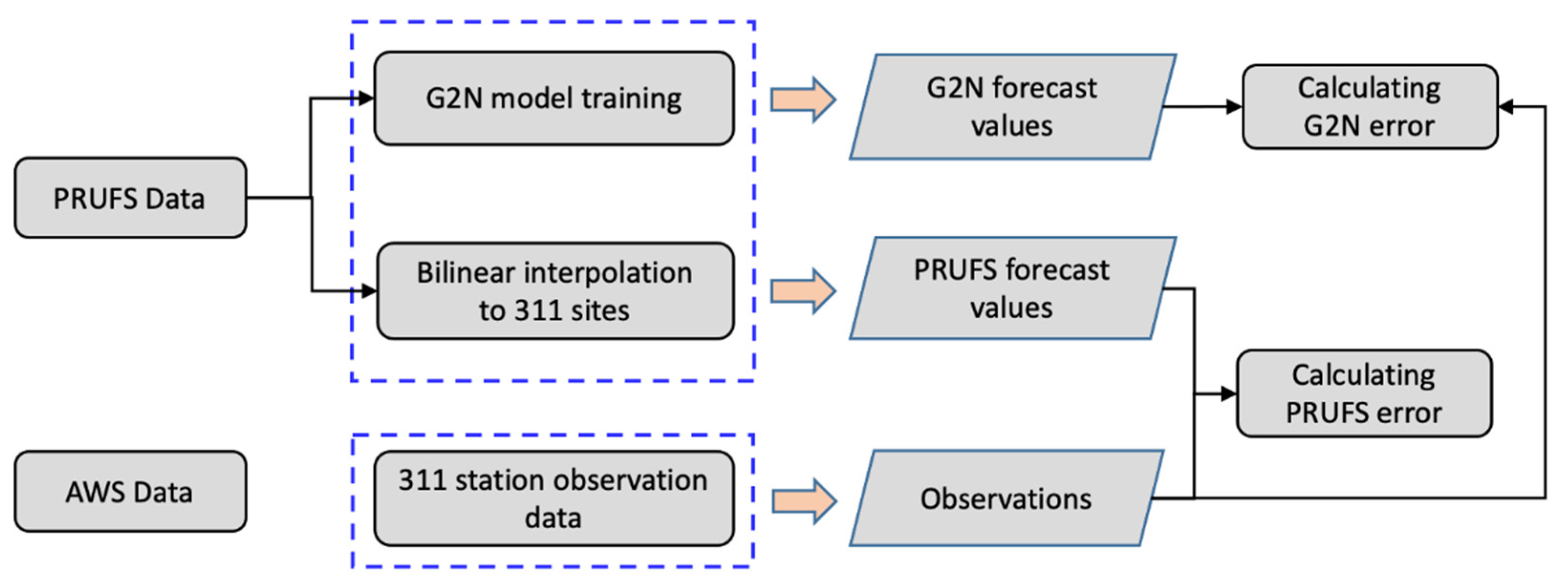
2. Data and Method
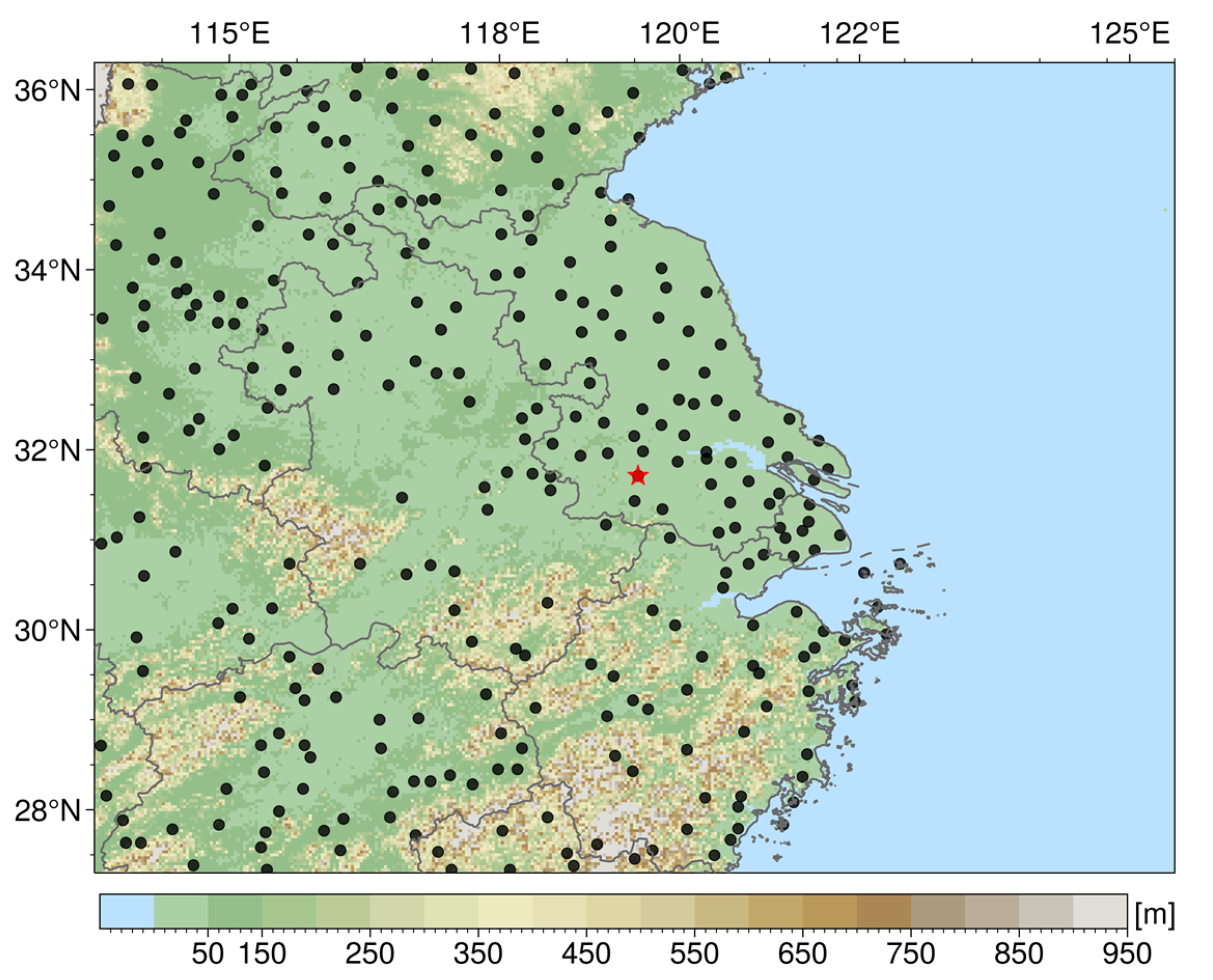
2.1. Data Description
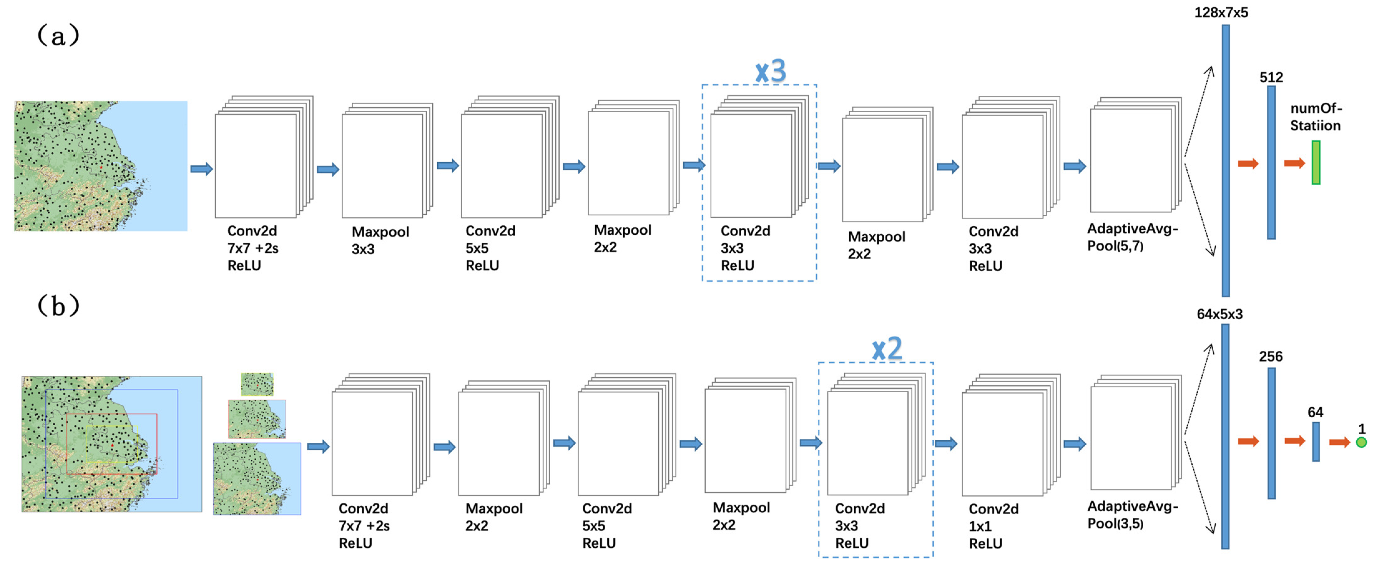
2.2. G2N Model
2.3. Data Pre-Processing and Dataset Partitioning
2.4. Model Evaluation Statistics
3. Results and Analysis
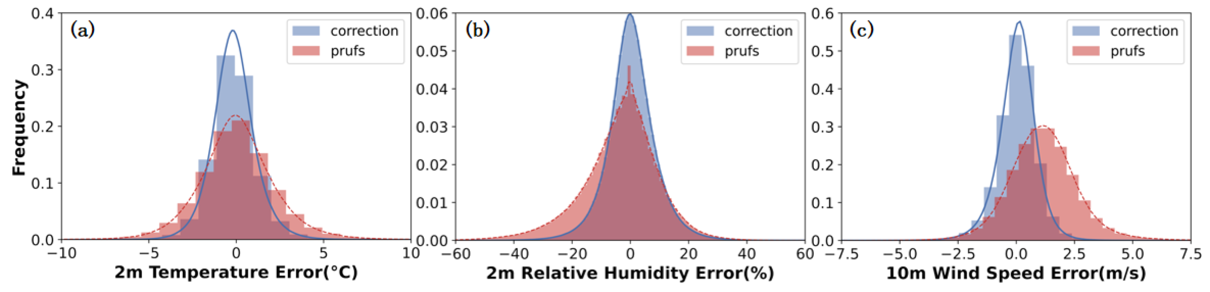
3.1. Overall Test Results
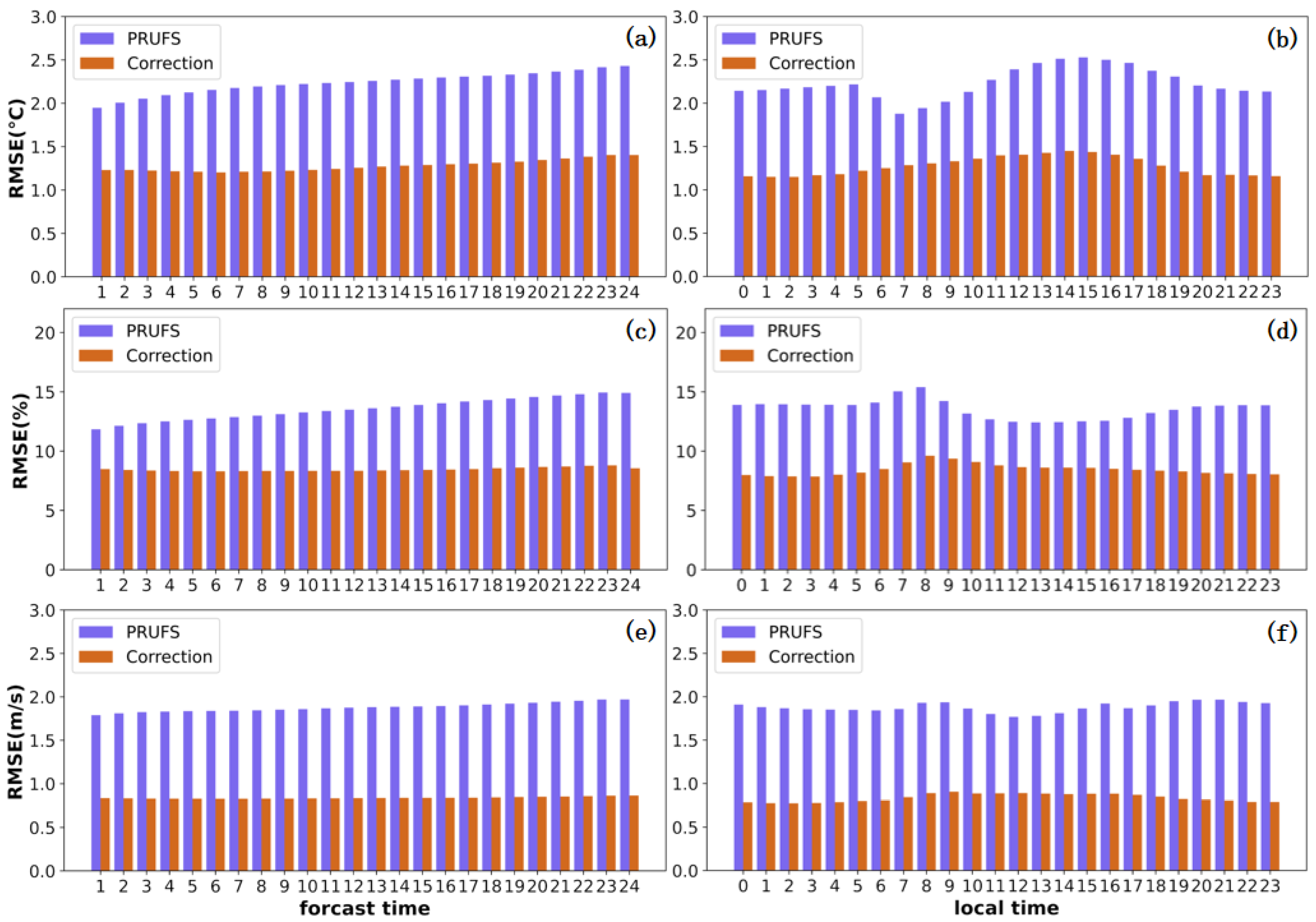
3.2. Forecast Lead Time and Daily Variation
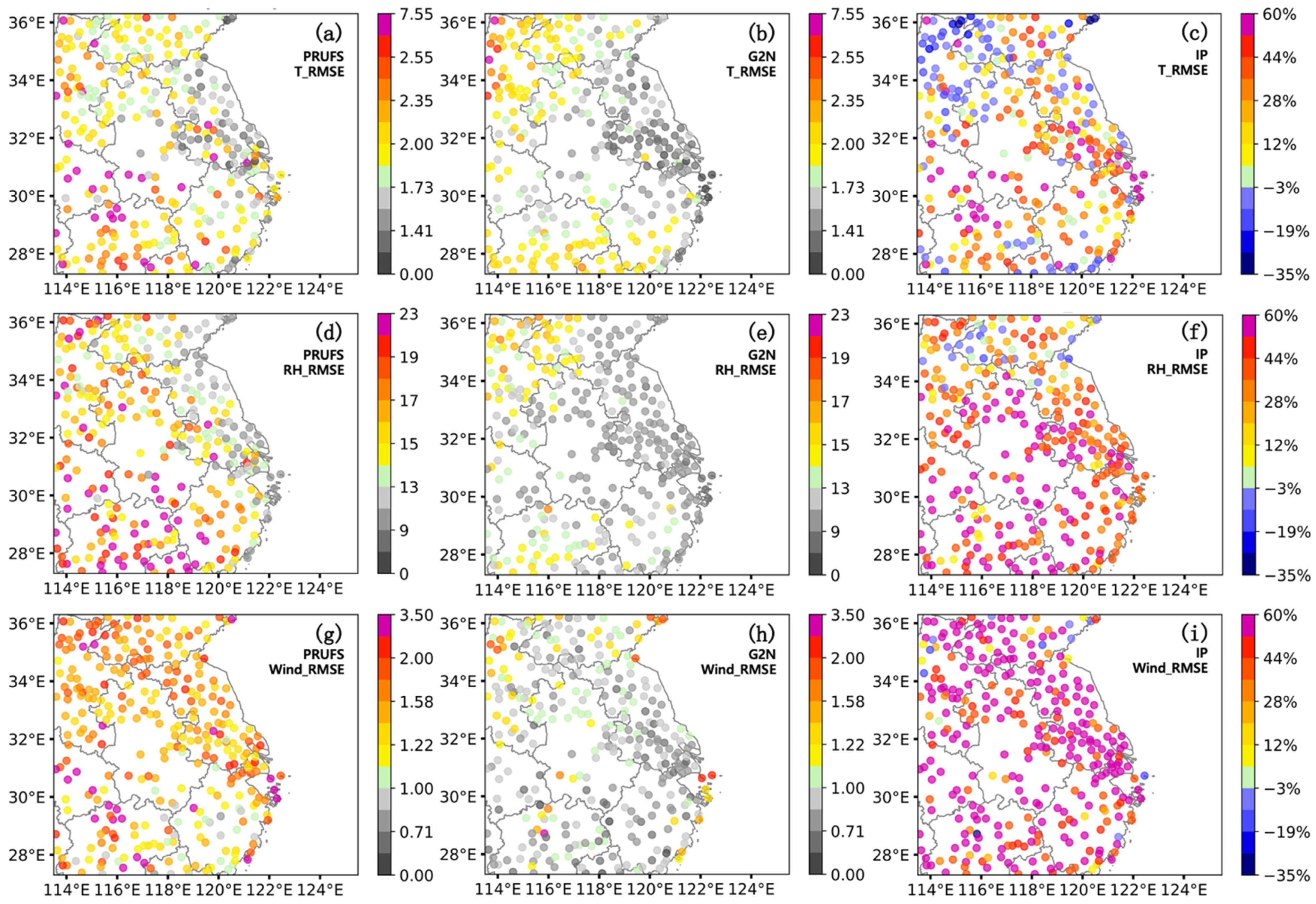
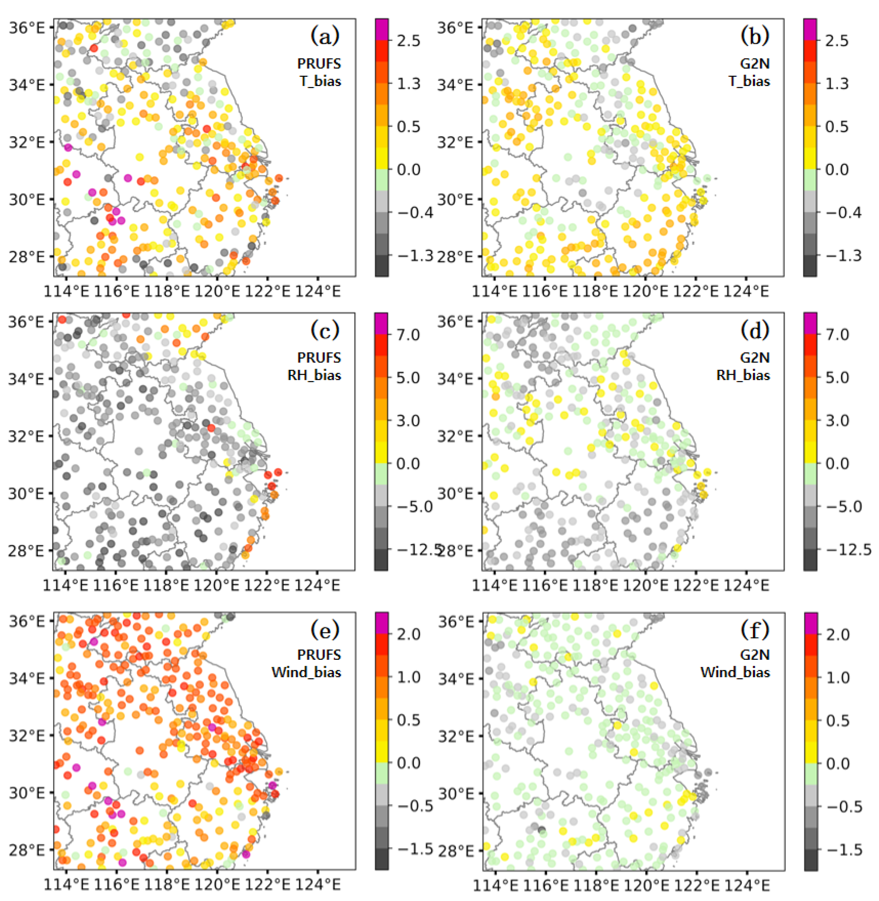
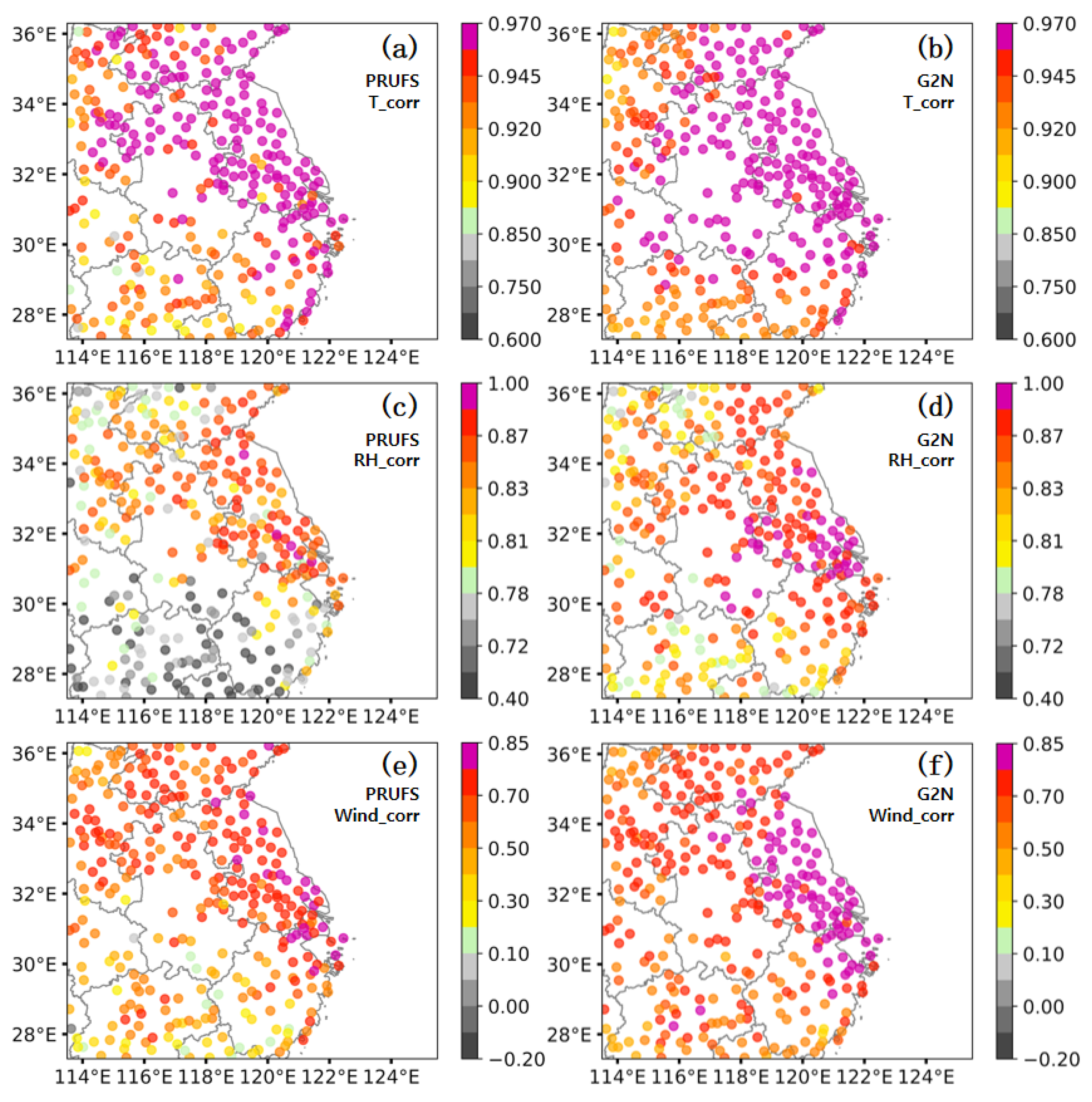
3.3. Spatial Distribution of the G2N Performances
4. Sensitivity Analysis of G2N to the Inputs and Learning Areas
4.1. Impact of the PRUFS Forecast Input (G-Exp)
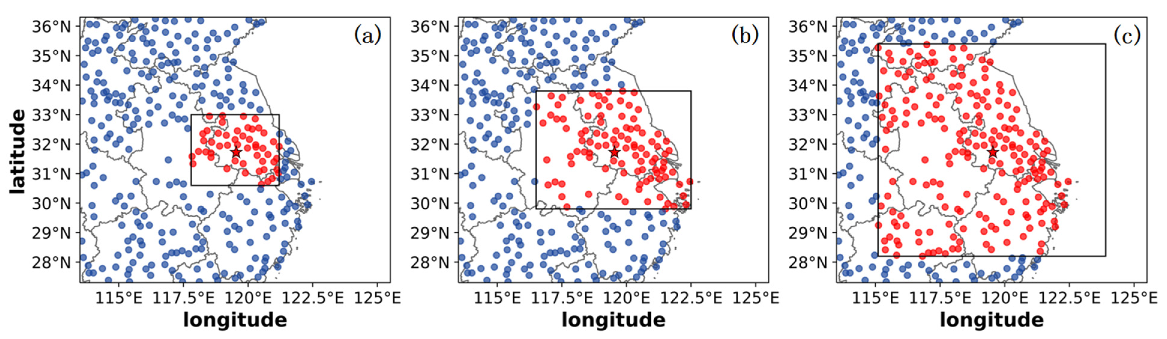
4.2. Impact of the Sites for Multitask Learning(N-Exp)
5. Conclusions
Author Contributions
Funding
Institutional Review Board Statement
Informed Consent Statement
Data Availability Statement
Acknowledgments
Conflicts of Interest
References
- Bauer, P.; Thorpe, A.; Brunet, G. The Quiet Revolution of Numerical Weather Prediction. Nature 2015, 525, 47–55. [Google Scholar] [CrossRef] [PubMed]
- Glahn, H.R.; Lowry, D.A. The Use of Model Output Statistics (MOS) in Objective Weather Forecasting. J. Appl. Meteorol. 1972, 11, 1203–1211. [Google Scholar] [CrossRef]
- Klein, W.H.; Lewis, B.M.; Enger, I. Objective prediction of five-day mean temperatures during winter. J. Meteorol. 1959, 16, 672–682. [Google Scholar] [CrossRef]
- Homleid, M. Diurnal Corrections of Short-Term Surface Temperature Forecasts Using the Kalman Filter. Weather Forecast. 1995, 10, 689–707. [Google Scholar] [CrossRef]
- Delle Monache, L.; Nipen, T.; Liu, Y.; Roux, G.; Stull, R. Kalman Filter and Analog Schemes to Postprocess Numerical Weather Predictions. Mon. Weather Rev. 2011, 139, 3554–3570. [Google Scholar] [CrossRef] [Green Version]
- Delle Monache, L.; Eckel, F.A.; Rife, D.L.; Nagarajan, B.; Searight, K. Probabilistic Weather Prediction with an Analog Ensemble. Mon. Weather Rev. 2013, 141, 3498–3516. [Google Scholar] [CrossRef] [Green Version]
- Alessandrini, S.; Davò, F.; Sperati, S.; Benini, M.; Delle Monache, L. Comparison of the Economic Impact of Different Wind Power Forecast Systems for Producers. Adv. Sci. Res. 2014, 11, 49–53. [Google Scholar] [CrossRef] [Green Version]
- Alessandrini, S.; Delle Monache, L.; Sperati, S.; Cervone, G. An Analog Ensemble for Short-Term Probabilistic Solar Power Forecast. Appl. Energy 2015, 157, 95–110. [Google Scholar] [CrossRef] [Green Version]
- Nagarajan, B.; Delle Monache, L.; Hacker, J.P.; Rife, D.L.; Searight, K.; Knievel, J.C.; Nipen, T.N. An Evaluation of Analog-Based Postprocessing Methods across Several Variables and Forecast Models. Weather Forecast. 2015, 30, 1623–1643. [Google Scholar] [CrossRef]
- Whan, K.; Schmeits, M. Comparing Area Probability Forecasts of (Extreme) Local Precipitation Using Parametric and Machine Learning Statistical Postprocessing Methods. Mon. Weather Rev. 2018, 146, 3651–3673. [Google Scholar] [CrossRef]
- Li, H.; Yu, C.; Xia, J.; Wang, Y.; Zhu, J.; Zhang, P. A Model Output Machine Learning Method for Grid Temperature Forecasts in the Beijing Area. Adv. Atmos. Sci. 2019, 36, 1156–1170. [Google Scholar] [CrossRef]
- Cho, D.; Yoo, C.; Im, J.; Cha, D. Comparative Assessment of Various Machine Learning-Based Bias Correction Methods for Numerical Weather Prediction Model Forecasts of Extreme Air Temperatures in Urban Areas. Earth Space Sci. 2020, 7, e2019EA000740. [Google Scholar] [CrossRef] [Green Version]
- Rasp, S.; Lerch, S. Neural Networks for Post-Processing Ensemble Weather Forecasts. Mon. Weather Rev. 2018, 146, 3885–3900. [Google Scholar] [CrossRef] [Green Version]
- Han, L.; Chen, M.; Chen, K.; Chen, H.; Zhang, Y.; Lu, B.; Song, L.; Qin, R. A Deep Learning Method for Bias Correction of ECMWF 24–240 h Forecasts. Adv. Atmos. Sci. 2021, 38, 1444–1459. [Google Scholar] [CrossRef]
- Zhang, Y.; Chen, M.; Han, L.; Song, L.; Yang, L. Multi-element deep learning fusion correction method for numerical weather prediction. Acta Meteorol. Sin. 2022, 80, 153–167. [Google Scholar]
- Skamarock, W.C.; Klemp, J.B.; Dudhia, J.; Gill, D.O.; Barker, D.M.; Duda, M.G.; Huang, X.-Y.; Wang, W.; Powers, J.G. A Description of the Advanced Research WRF Version 3; National Center for Atmospheric Research: Boulder, CO, USA, 2008. [Google Scholar]
- Krizhevsky, A.; Sutskever, I.; Hinton, G.E. ImageNet Classification with Deep Convolutional Neural Networks. Commun. ACM 2017, 60, 84–90. [Google Scholar] [CrossRef] [Green Version]
- Shimodaira, H. Improving Predictive Inference under Covariate Shift by Weighting the Log-Likelihood Function. J. Stat. Plan Inference 2000, 90, 227–244. [Google Scholar] [CrossRef]
- Ioffe, S.; Szegedy, C. Batch Normalization: Accelerating Deep Network Training by Reducing Internal Covariate Shift. Proc. Mach. Learn. Res. 2015, 37, 448–456. [Google Scholar]
- Rahaman, N.; Baratin, A.; Arpit, D.; Draxler, F.; Lin, M.; Hamprecht, F.A.; Bengio, Y.; Courville, A. On the Spectral Bias of Neural Networks. Proc. Mach. Learn. Res. 2018, 97, 5301–5310. [Google Scholar]
- Pan, L.; Liu, Y.; Roux, G.; Cheng, W.; Liu, Y.; Hu, J.; Jin, S.; Feng, S.; Du, J.; Peng, L. Seasonal Variation of the Surface Wind Forecast Performance of the High-Resolution WRF-RTFDDA System over China. Atmos. Res. 2021, 259, 105673. [Google Scholar] [CrossRef]
- Shi, J.; Liu, Y.; Li, Y.; Liu, Y.; Roux, G.; Shi, L.; Fan, X. Wind Speed Forecasts of a Mesoscale Ensemble for Large-Scale Wind Farms in Northern China: Downscaling Effect of Global Model Forecasts. Energies 2022, 15, 896. [Google Scholar] [CrossRef]
- Zeng, X.-M.; Wang, M.; Wang, N.; Yi, X.; Chen, C.; Zhou, Z.; Wang, G.; Zheng, Y. Assessing Simulated Summer 10-m Wind Speed over China: Influencing Processes and Sensitivities to Land Surface Schemes. Clim. Dyn. 2018, 50, 4189–4209. [Google Scholar] [CrossRef]
- Minton, P.D.; Cohen, J. Statistical Power Analysis for the Behavioral Sciences. J. Am. Stat. Assoc. 1971, 66, 428. [Google Scholar] [CrossRef]
- Cohen, J. Statistical Power Analysis for the Behavioral; Routledge: London, UK, 1988. [Google Scholar]
- Kumar, A.; Daumé, H., III. Learning Task Grouping and Overlap in Multi-Task Learning. arXiv 2012, arXiv:1206.6417. [Google Scholar]
- Gao, Y.; Ma, J.; Zhao, M.; Liu, W.; Yuille, A.L. NDDR-CNN: Layerwise Feature Fusing in Multi-Task CNNs by Neural Discriminative Dimensionality Reduction. In Proceedings of the 2019 IEEE/CVF Conference on Computer Vision and Pattern Recognition (CVPR), Long Beach, CA, USA, 15–20 June 2019; pp. 3200–3209. [Google Scholar]
- Crawshaw, M. Multi-Task Learning with Deep Neural Networks: A Survey. arXiv 2020, arXiv:2009.09796. [Google Scholar]
- Li, Y.; Lang, J.; Ji, L.; Zhong, J.; Wang, Z.; Guo, Y.; He, S. Weather Forecasting Using Ensemble of Spatial-Temporal Attention Network and Multi-Layer Perceptron. Asia Pac. J. Atmos. Sci. 2021, 57, 533–546. [Google Scholar] [CrossRef]


| Element | Test Dataset | ||
|---|---|---|---|
| PRUFS | G2N | IP | |
| 2 m-T | 2.22 | 1.79 | 19.4% |
| 2 m-RH | 16.25 | 12.27 | 24.5% |
| 10 m-WD | 1.66 | 0.95 | 42.8% |
| AreaRatios of Input Domain | PRUFS Forecasts (RMSE)-“Jintan” | G2-One Correction (RMSE)-“Jintan” | IP | PRUFS Forecasts (RMSE)-“Nanjing” | G2-One Correction (RMSE)-“Nanjing” | IP |
|---|---|---|---|---|---|---|
| 1.0 (G2N331) | 1.47 | 0.89 | 39.5% | 1.36 | 0.97 | 28.7% |
| 1.0 | 1.48 | 0.98 | 33.8% | 1.37 | 1.05 | 23.4% |
| 0.9 | 1.48 | 0.96 | 35.1% | 1.37 | 1.04 | 24.1% |
| 0.8 | 1.48 | 0.96 | 35.1% | 1.37 | 1.02 | 25.5% |
| 0.7 | 1.48 | 0.90 | 39.2% | 1.37 | 0.98 | 28.5% |
| 0.6 | 1.48 | 0.97 | 34.5% | 1.37 | 1.01 | 26.3% |
| 0.5 | 1.48 | 0.97 | 34.5% | 1.37 | 1.01 | 26.3% |
| 0.4 | 1.48 | 0.98 | 33.8% | 1.37 | 1.02 | 25.5% |
| 0.3 | 1.48 | 0.98 | 33.8% | 1.37 | 1.02 | 25.5% |
| (a) 2 m Temperature Statistics Results | |||||
|---|---|---|---|---|---|
| Verification | 51 | 101 | 199 | 311 | |
| N-exps | |||||
| G2N51 | 16.4% | ||||
| G2N101 | 14.1% | 13.8% | |||
| G2N199 | 19.8% | 19.8% | 21.8% | ||
| G2N311 | 20.8% | 20.2% | 21.8% | 18.9% | |
| (b) 2 m Relative Humidity Statistics Results | |||||
| Verification | 51 | 101 | 199 | 311 | |
| N-exps | |||||
| G2N51 | 23.7% | ||||
| G2N101 | 24% | 25.5% | |||
| G2N199 | 25.7% | 27.5% | 24.6% | ||
| G2N311 | 27.8% | 28.9% | 25.7% | 24.5% | |
| (c) 10 m Wind Speed Statistics Results | |||||
| Verification | 51 | 101 | 199 | 311 | |
| N-exps | |||||
| G2N51 | 44.5% | ||||
| G2N101 | 46.5% | 43.4% | |||
| G2N199 | 44.5% | 41.6% | 40.9% | ||
| G2N311 | 47.4% | 44% | 43.9% | 42.8% | |
Disclaimer/Publisher’s Note: The statements, opinions and data contained in all publications are solely those of the individual author(s) and contributor(s) and not of MDPI and/or the editor(s). MDPI and/or the editor(s) disclaim responsibility for any injury to people or property resulting from any ideas, methods, instructions or products referred to in the content. |
© 2023 by the authors. Licensee MDPI, Basel, Switzerland. This article is an open access article distributed under the terms and conditions of the Creative Commons Attribution (CC BY) license (https://creativecommons.org/licenses/by/4.0/).
Share and Cite
Qin, Y.; Liu, Y.; Jiang, X.; Yang, L.; Xu, H.; Shi, Y.; Huo, Z. Grid-to-Point Deep-Learning Error Correction for the Surface Weather Forecasts of a Fine-Scale Numerical Weather Prediction System. Atmosphere 2023, 14, 145. https://doi.org/10.3390/atmos14010145
Qin Y, Liu Y, Jiang X, Yang L, Xu H, Shi Y, Huo Z. Grid-to-Point Deep-Learning Error Correction for the Surface Weather Forecasts of a Fine-Scale Numerical Weather Prediction System. Atmosphere. 2023; 14(1):145. https://doi.org/10.3390/atmos14010145
Chicago/Turabian StyleQin, Yu, Yubao Liu, Xinyu Jiang, Li Yang, Haixiang Xu, Yueqin Shi, and Zhaoyang Huo. 2023. "Grid-to-Point Deep-Learning Error Correction for the Surface Weather Forecasts of a Fine-Scale Numerical Weather Prediction System" Atmosphere 14, no. 1: 145. https://doi.org/10.3390/atmos14010145