1. Introduction
The difference in ionospheric delay of the two carrier waves from the GNSS satellite can be used to study ionosphere characteristics in the form of total electron content. TEC represents the electron density in the ionosphere layer along the line-of-sight (LoS) between the satellite and the receiver on the earth’s surface. The electron density experiences disturbance from deformation due to earthquakes [
1]. These disturbances are known as co-seismic ionospheric disturbances. Plate movements caused by earthquakes can trigger the formation of acoustic waves. Furthermore, the acoustic waves will propagate toward the ionosphere layer within a few minutes after the earthquake.
The first CID observation using GNSS-TEC was carried out by Calais and Minster [
2], and Rolland et al. [
3] developed observations to obtain the mechanism of the directivity of CID. Cahyadi & Heki [
4] observed the CID that occurred in the 2007 Bengkulu earthquake, which was detected 11–16 min after mainshock with a speed of ~0.7 km/s. Furthermore, it occurred in the 2012 North Sumatra earthquake, which was detected 10–15 min after the earthquake with an acoustic wave velocity of 0.8–1.0 km/s. This observation also introduces the empirical relationship between earthquake magnitude and CID amplitude. Cahyadi et al. [
5] observed CID that occurred in the 2016 West Sumatra and 2018 Palu earthquakes. It was detected 10–15 min after the earthquake, with large TEC amplitudes reaching 2.9 TECU and 0.4 TECU, as well as speeds of ~1–1.72 km/s and ~0.97–1.08 km/s. Sumatra’s earthquake studies in 2005 [
6] and 2004 [
7] also provide insightful analysis. However, several previous similar studies have focused on the movement of CID in the two dimensions observed based on a time series of STEC (Slant Total Electron Content) changes. In this research, we continue the research of Cahyadi et al. [
5] by investigating the direction of movement (directivity) of the ionospheric disturbance caused by the earthquake. We analyze multi-temporal with time interval every minute.
The refinement of the CID spatial distribution analysis was conducted by Cahyadi et al. [
8], which observed the 2020 Turkey earthquake. These observations provide an overview of the spatial distribution found in detail from an altitude of 100–600 km. However, the less dense network of GNSS observation stations causes the CID movement to appear inefficient. Cahyadi et al. [
5] observed the CID in the 2016 West Sumatra earthquake to collect information on the CID detected after the mainshock and obtain the speed of acoustic waves and crustal deformation. Nevertheless, the resulting analysis only detects ionospheric disturbances at an altitude of 300 km in two dimensions. Rahayu et al. [
9] also comprehensively observed the earthquake, but the data used cannot analyze spatial distribution. Cahyadi et al. [
10] succeed to analyze CID and the directivity of propagation as 3D tomography in the 2018 Palu earthquake. The epicenter of the earthquake was in the equatorial region, where an anomaly was found moving to the south. However, this research needs to be improved to analyze the directivity of anomaly propagation in southern hem-isphere. Therefore, this study analyzes ionospheric disturbances spatial distribution (each ionosphere altitude layer) in the 2016 West Sumatra earthquake which is located in the southern hemisphere with larger magnitude of earthquake.
Additional observations on the spatial structure and temporal evolution of the CID electron density anomaly are needed to effectively understand the underlying physical processes. He and Heki [
11] studied the spatial structure of the electron density anomaly before the 2015 Illapel earthquake, Chile (Mw 8.3), using 3D tomography techniques. The results showed that the preseismic changes consisted of two parts: the increase and decrease in ionospheric electron density. The anomalies appeared ~20 min before the earthquake and were located at lower and higher elevations with the geomagnetic field. The study focused on preseismic anomalies, while this paper analyzes co-seismic anomalies. The same 3D tomography technique has been applied to studying the 3D structure of electron density changes by the 2017 total eclipse in North America [
12] and the E-sporadic irregularity in Japan [
13]. In addition, it performed a CID spatial analysis using a 3D tomography technique to observe changes in the ionospheric density through GPS observations from the Indonesia Continuously Operating Reference Station (InaCORS) and Sumatran GPS Array (SUGAR).
2. Dataset and Methodology
2.1. GNSS Data
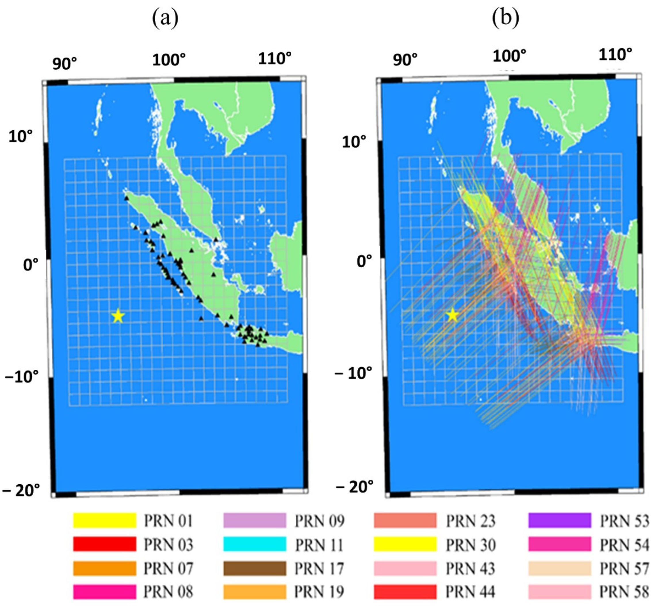
GNSS data from InaCORS and SUGAR stations were used in this study. InaCORS is a network of Continuously Operating Reference Station (CORS) GNSS stations in Indonesia, while SUGAR is of CORS GNSS stations spread across Sumatra Island and its surroundings. The 67 stations were used in total, consisting of InaCORS and SUGAR spread across Sumatra Island to study ionospheric anomalies. Satellites GPS PRN 01, 03, 07, 08, 09, 11, 17, 19, 23, 30, and GLONASS PRN 43, 44, 53, 54, 57, 58 observed the ionospheric conditions surrounding the epicenter.
The GNSS phase difference between L1 (~1.5 GHz) and L2 (~1.2 GHz) has been changed to STEC.
Figure 1 (right) provides an overview of the LoS found in GPS observations around the earthquake epicenter. The LoS also determines the STEC value employed to reconstruct the 3D tomography model. Furthermore, a high-pass filter is used to eliminate bias due to the movement of the satellite during the orbit. Typically done by the polynomial reference curve to obtain the CID signal detected when there is a significant peak at the time series of residual STEC value [
4]. This reference curve method is suitable for studying signals because the nature of the CID signal due to an earthquake will not leave a permanent value change in the TEC. To determine the spatial characteristics of the CID, such as perturbation velocity, a point calculation of the line of sight has been carried out, assuming the ionosphere as a thin layer with a height of ~300 km or Ionospheric Piercing Point (IPP). The behavior of ionospheric TEC was investigated immediately after a significant earthquake by comparing it with TEC before and after a series of earthquake-related disturbances.
The density of the number of receivers from the two groups of stations used can analyze the movement of the CID in three dimensions. The movement observed in three dimensions can be seen with a tight receiver density based on asymmetry theory [
14].
2.2. Voxel Setup
For the 3D tomography model, the voxel was set up over Sumatra Island. The voxel block dimensions we modeled based on trial and error and the best results were when we set the block size to 1° × 1.2° × 75 km. The electron density in the block is assumed to be homogeneous. One LoS can penetrate several blocks, and the residual STEC can be described as the sum of the anomalous values of each penetration length and electron density. The penetration length was calculated from a distance between two intersections on the block surface by simple geometry assuming that the earth is a sphere (the ellipticity is neglected) with an average radius.
In this study, the tomographic model that we use uses two types of constraints, namely continuity constraints and high-dependent constraints. The 3D tomography model will be able to represent the ionosphere picture perfectly when LoS can be distributed densely in each voxel. However, there are limitations to the uneven distribution of LoS when the research area is above the sea area. This can be solved using a continuity constraint to assume that neighboring voxels have relatively the voxels passed by LoS with the assumption of 0.10 × 10
11 el/m
3 as an allowance. The uniform STEC error was assumed as 0.2 TECU with 1 TECU is 10
16 el/m
2 [
15], while high- dependent constraints are used to provide more realistic modeling results. This is to avoid estimation of unrealistically large electron density anomalies in very high or very low altitudes [
16]. We are using the Chapman model in our height-dependent constraints. The constraints assumed that the maximum ionization in altitude is ~300 km.
The local ionosphere was divided into three-dimensional voxel grids to perform 3-D tomography of the ionospheric electron density anomaly. Each voxel is limited to latitude, longitude, and altitude, and the electron density anomaly is assumed to be homogeneous. Observation of absolute STEC anomaly (ΔSTECi) with each beam path is estimated as the number of electron density anomaly products per unit length and voxel penetration length [
10]:
is the total number of voxels,
and
are the beam path length and electron density of the
voxels, and
is the observed and approximate errors. Equation (1) can be expressed in matrix form as follows when the total number of line-of-sights (LOS) is m [
10]:
where Y and E are observation vectors and error vectors with m elements, respectively. The Jacobian matrix with m × n components is denoted by A, and X is the electron density anomaly of n voxels to be estimated.
2.3. Resolution Setup
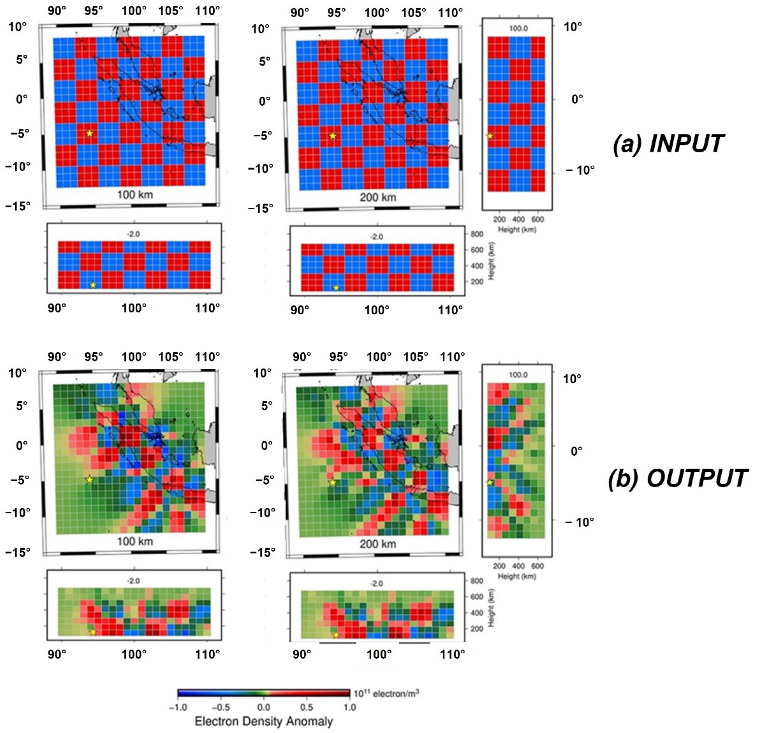
The accuracy of 3D tomography can be assessed by performing inversions to recover the artificial distribution of the electron density anomaly using synthetic data. First, the resolution test was performed with the classic checkerboard pattern. Meanwhile, the same satellite and station geometry was assumed 15 min after the earthquake to synthesize the input STEC data for 3D tomography.
Figure 2 (input) shows that the assumed checkerboard pattern consists of an electron density anomaly of ±0.5 TECU/100 km. The anomaly was allowed to change incrementally between the positive and negative halves to make the pattern consistent with the continuity constraint. The anomalous amplitudes are also assumed to decay at very high and low ionospheres to be compatible with other constraints.
Figure 2b shows the recovered pattern for blocks at an elevation range of 100 and 200 km. This pattern recovered well, especially on the mainland, which is Sumatra Island, and the offshore GNSS stations are very limited. Insufficient coverage of stations over the ocean is an inherent weakness of such studies as large earthquakes occur near land-sea boundaries.
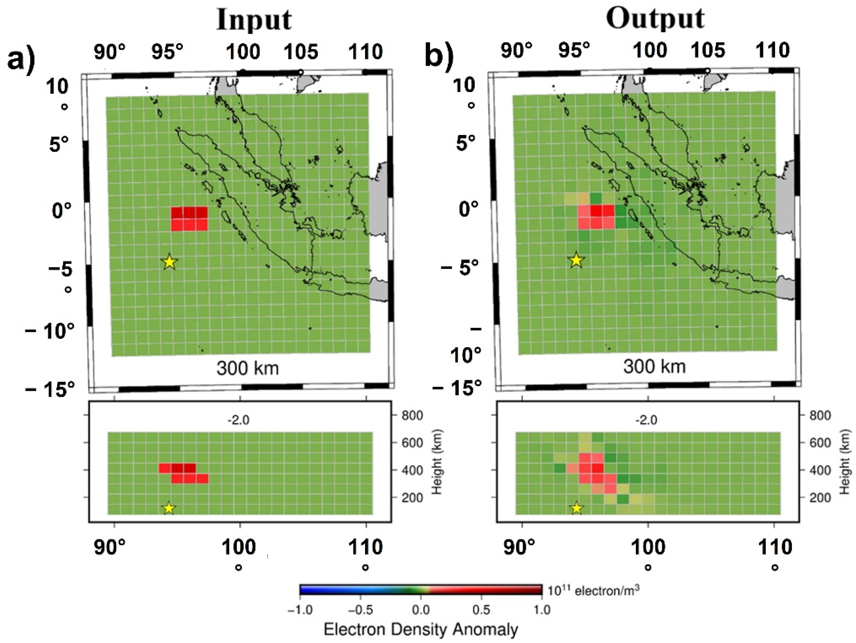
The reliability of the tomographic model for the subsequent discussion of electron density anomalies was assessed by recovering a pattern consisting of a pair of positive and negative anomalies (0.6 × 10
11 el/m
3) at low and high altitudes, respectively on a neutral background as indicated in
Figure 3 input. The outcome as illustrated in
Figure 3 output reproduces the predicted pattern of the positive anomaly, with the amplitude of the input model decreased to 2/3 due to limitations. Similarly, the pattern of positive and negative anomalies in the latitude profile recovered well, with only weak smears in the surrounding blocks not exceeding a few percent of the assumed anomalies.
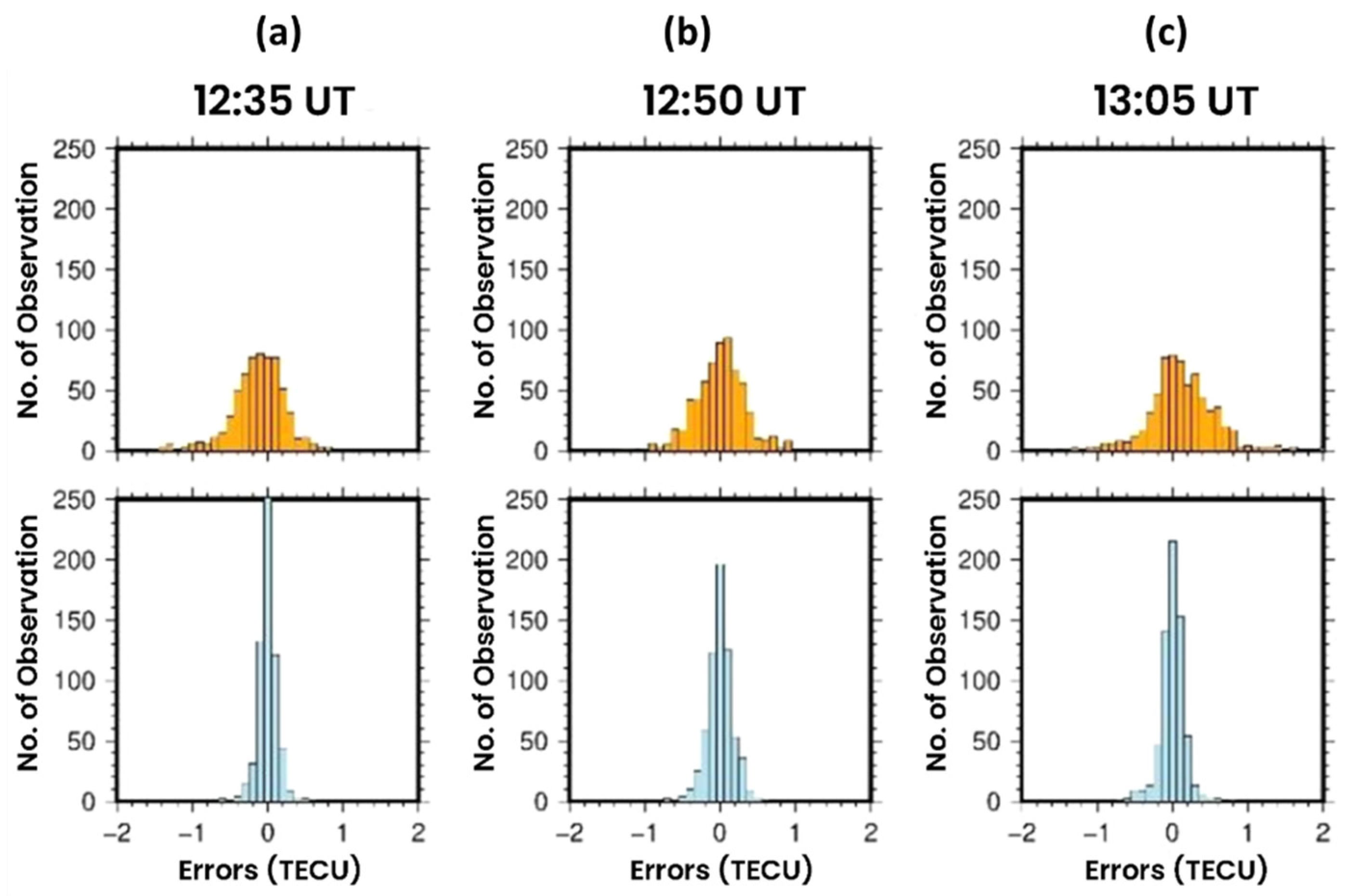
For additional accuracy assessments, raw STEC anomaly (upper panel) and STEC post-fit residual data were assessed (lower panel). Raw STEC anomaly data are obtained from the deviation value of STEC to the reference curve. In contrast, calculated STEC anomaly data are derived from the estimated electron density anomaly in all voxels along LoS.
Figure 4 is a histogram using raw and computed STEC anomaly data. Raw STEC anomaly data have a wide variance coverage around zero (12:35 UT = −1.4675 − 0.8476; 12:50 UT = −1.2807 − 0.9413; 13:05 UT = −1.5839 − 2.051). Meanwhile, calculated STEC anomaly data demonstrated substantially less dispersion around zero (12:35 UT = −0.6284 − 0.5741; 12:50 UT = −0.7386 − 0.6172; 13:05 UT = −0.7434 − 0.7852). This shows that the estimated 3D distribution of the anomaly explains the observed STEC well.
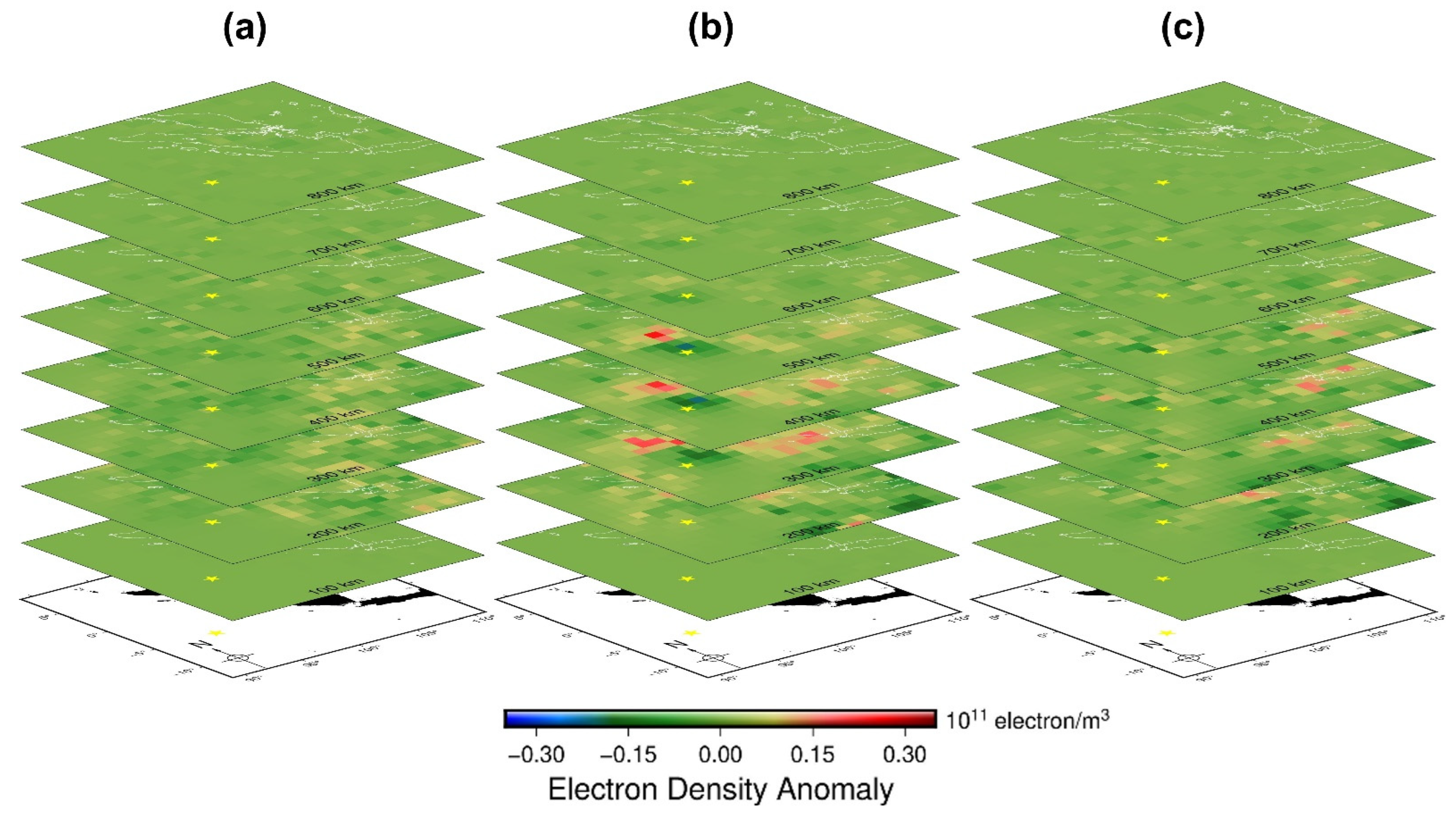
3. 3D Tomography Model
Figure 5 shows the map view of the researched 3D tomography for the altitude of 100–800 km at 16 min (13:06) after the 2016 Sumatra earthquake, with longitude and latitude profiles. It was confirmed earlier that the tomography performance remained high all this time. The results show that a strong positive electron density anomaly occurs in the 200–400 km altitude layer. The anomaly grows large without noticeable pattern changes or spatial deviations toward the mainshock. The latitude of the voxels showing the largest positive anomaly remained around 95° E over the 15 min.
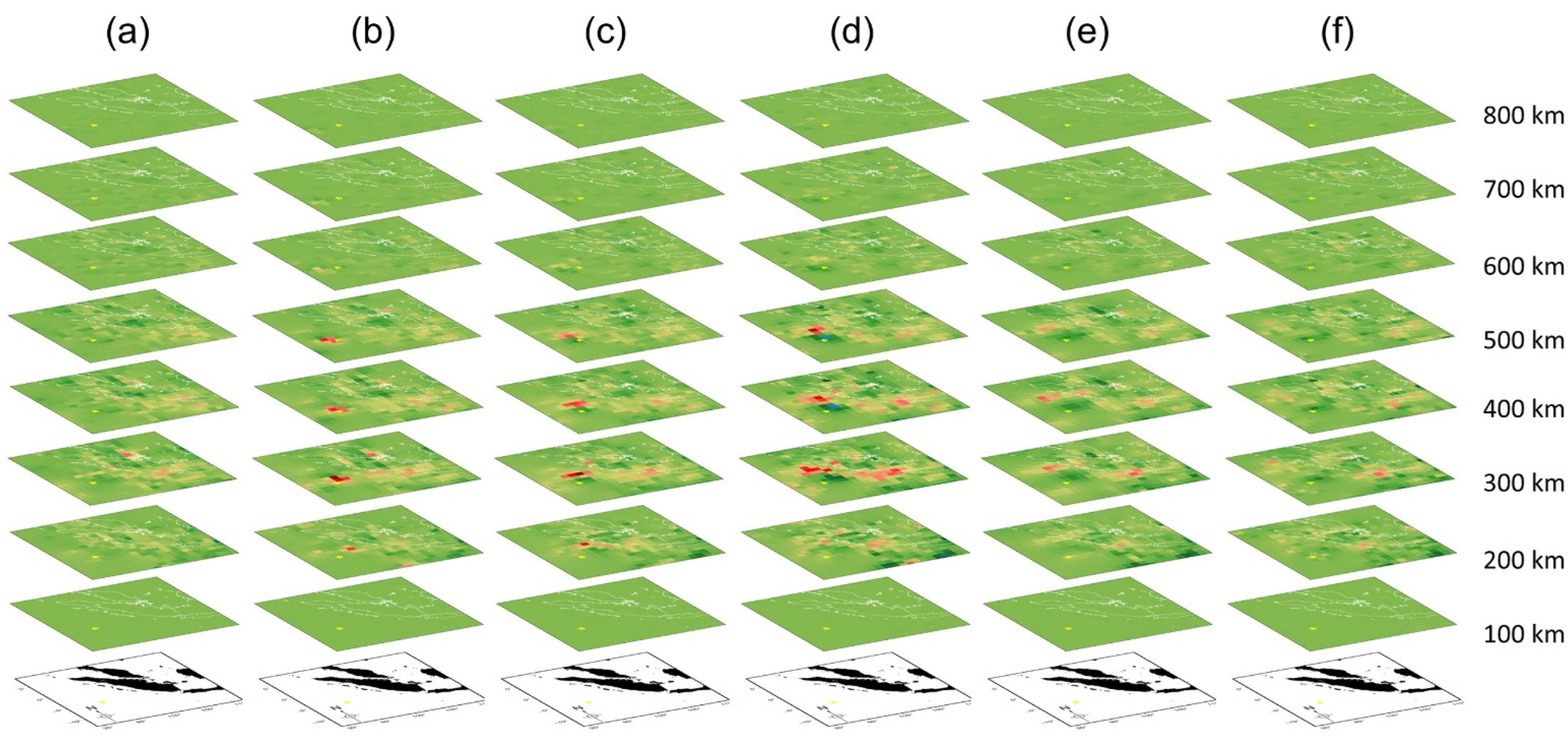
Figure 6 presents tomographic results for eight layers at an altitude of 100–800 km from 13:00 UT to 13:10 UT, and the earthquake occurred at 12:50. The anomaly began to be seen at 13:00 UT, approximately 10 min after the earthquake. The maximum anomaly was seen at 13:02 UT at an altitude of 300 km, which corresponds to the theory with the maximum ionization layer at an altitude of 300 km. The positive anomaly appears at an altitude of 300 km and moves to the southeast and northwest in its propagation. In the CID 3D tomography model, we observe that the positive anomaly is seen at lower altitudes (~200–300 km), while the negative one is seen at higher altitudes (~400–500 km), as shown in
Figure 6. The negative electron anomaly is located in the southern latitude of the positive one. The anomaly grows large without significant pattern changes or spatial deviations. A positive anomaly of CID propagation was seen 8 min after the appearance of the first at 13:02 UT. The emergence of a positive anomaly in this type of strike-slip earthquake is in accordance with observations [
1]. In addition, the observations of Heki [
15] show that positive anomalies generally occur at low altitudes (~100–300 km), while negative anomalies occur at high altitudes (~500–600 km). The positive anomaly moves toward the north, the movement is in accordance with observations (Heki & Ping [
14]) related to the movement of electric particles in acoustic waves that move closer to geomagnetic fields.
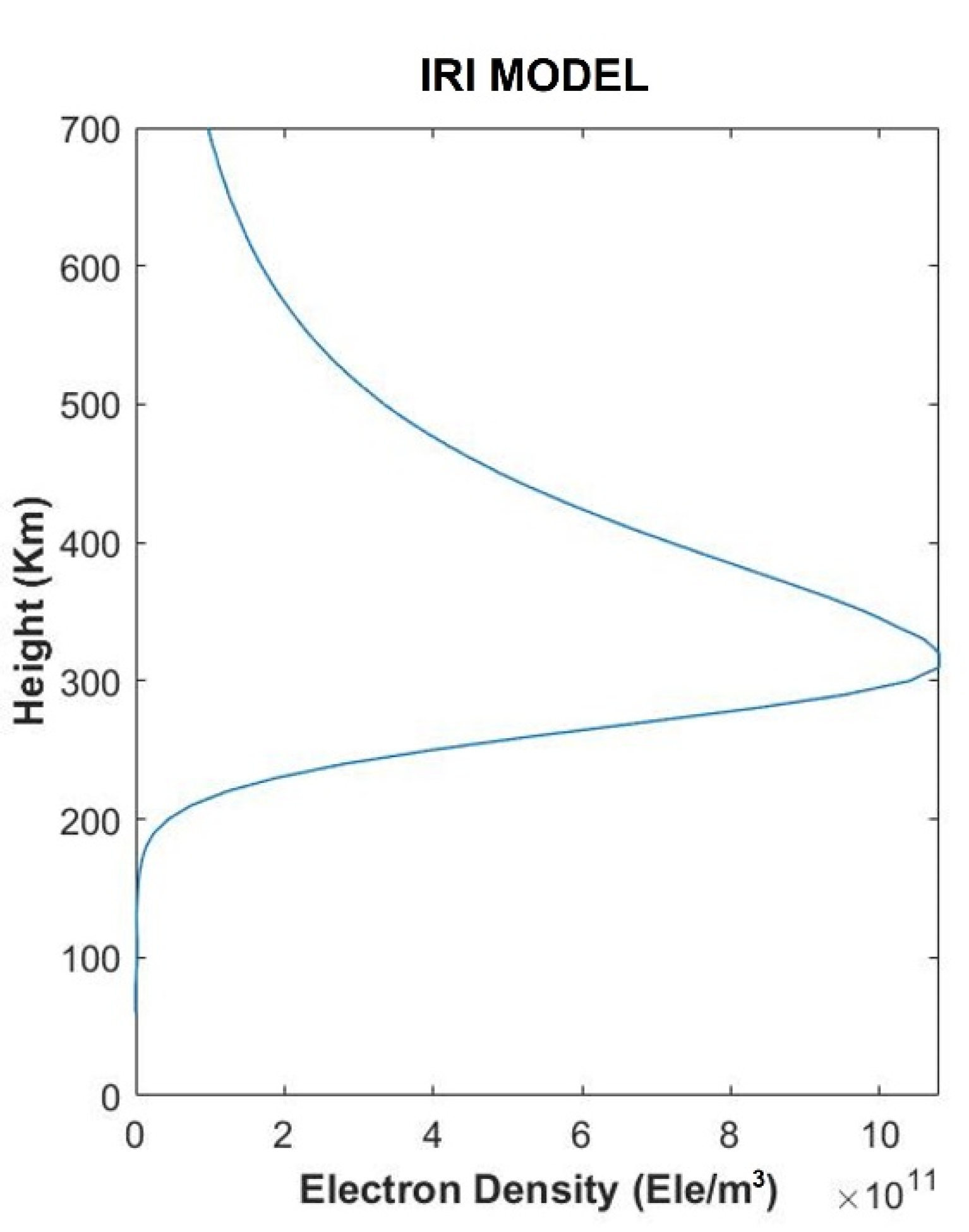
We also estimated the vertical profile of electron density using the IRI model (
https://irimodel.org/) on 2 March 2016. The CID occurred at 12.06 UT to prove that our model is realistic to the electron density profile of the IRI model. The primary IRI data are obtained from the ionosondes network around the world, powerful incoherent scatter radars, the ISIS (International Satellites for Ionospheric Studies) and Alouette topside sounders, and tools to obtain in situ data by launching satellites and rockets [
17]. The IRI model shows that the highest electron density is located at an altitude of ~300 km, as shown in
Figure 7, which supports 3D tomographic modeling, which is modeled at the height of the third ionospheric layer with an altitude of ~300 km [
18]. The configuration of IRI Model at altitude ~300 km was confirmed as shown in
Figure S1.
4. Discussion
We modeled the 3D tomography to obtain the spatial distribution of ionospheric anomalies caused by the earthquake. We perform the analysis at an altitude of 100–600 km according to
Figure 5. It can be seen in
Figure 5b, the anomaly is very clear in this 3D tomography modeling. While
Figure 5c shows the 3D tomography model returned to normal after CID propagated. To get a clear picture of the movement of CID, we show it in
Figure 6. In
Figure 6 it can be seen that CID begins to appear at 13:03 UT, where the emergence of CID is close to the epicenter location. Then the CID moves to the north, and disappears at 13:11 UT, the disappearance of this CID is based on the local nature of the CID anomaly. The movement can clearly be seen in
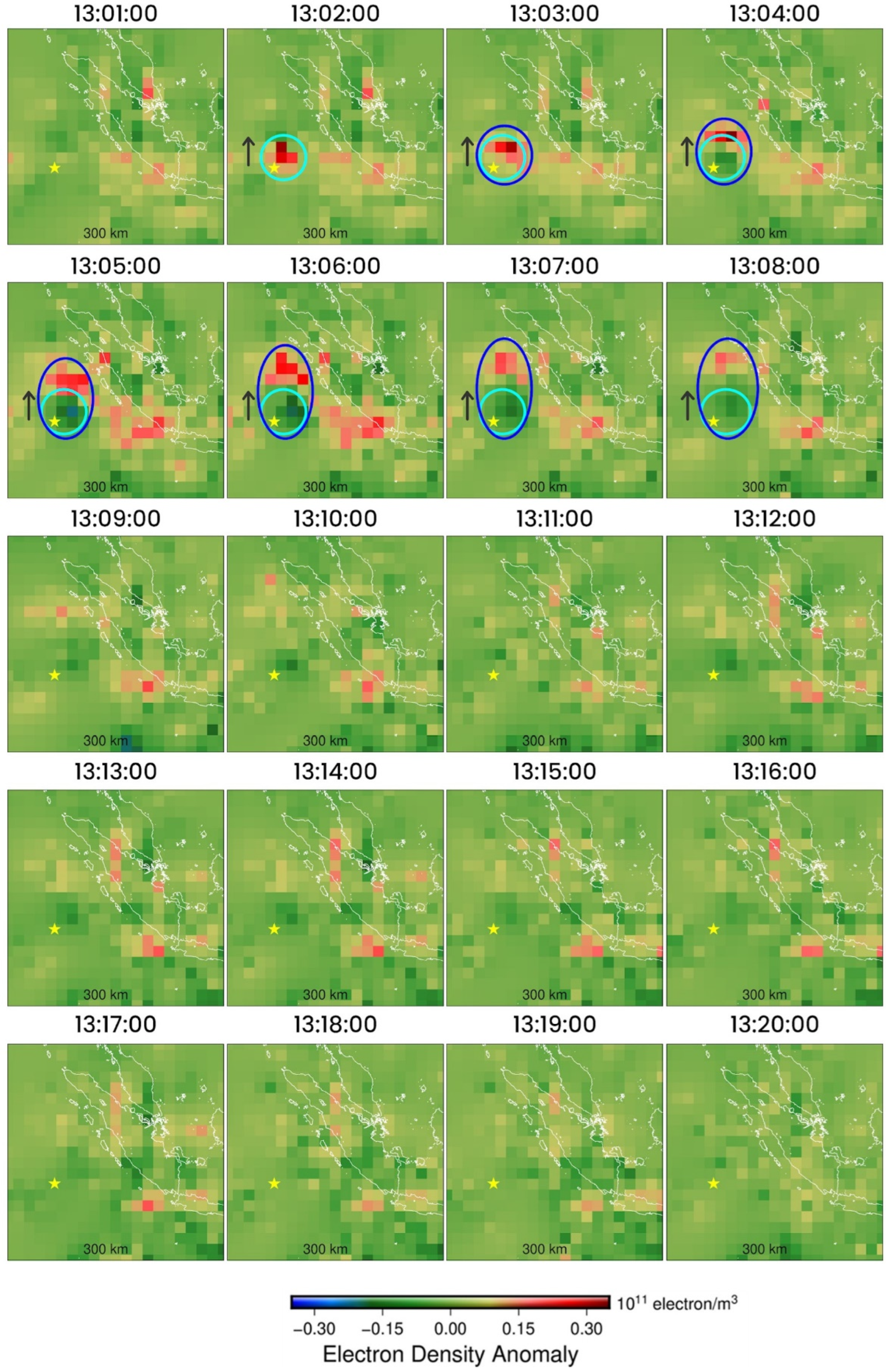
Figure 8, where we observed at an altitude of 300 km, where the anomalous values are dominant.
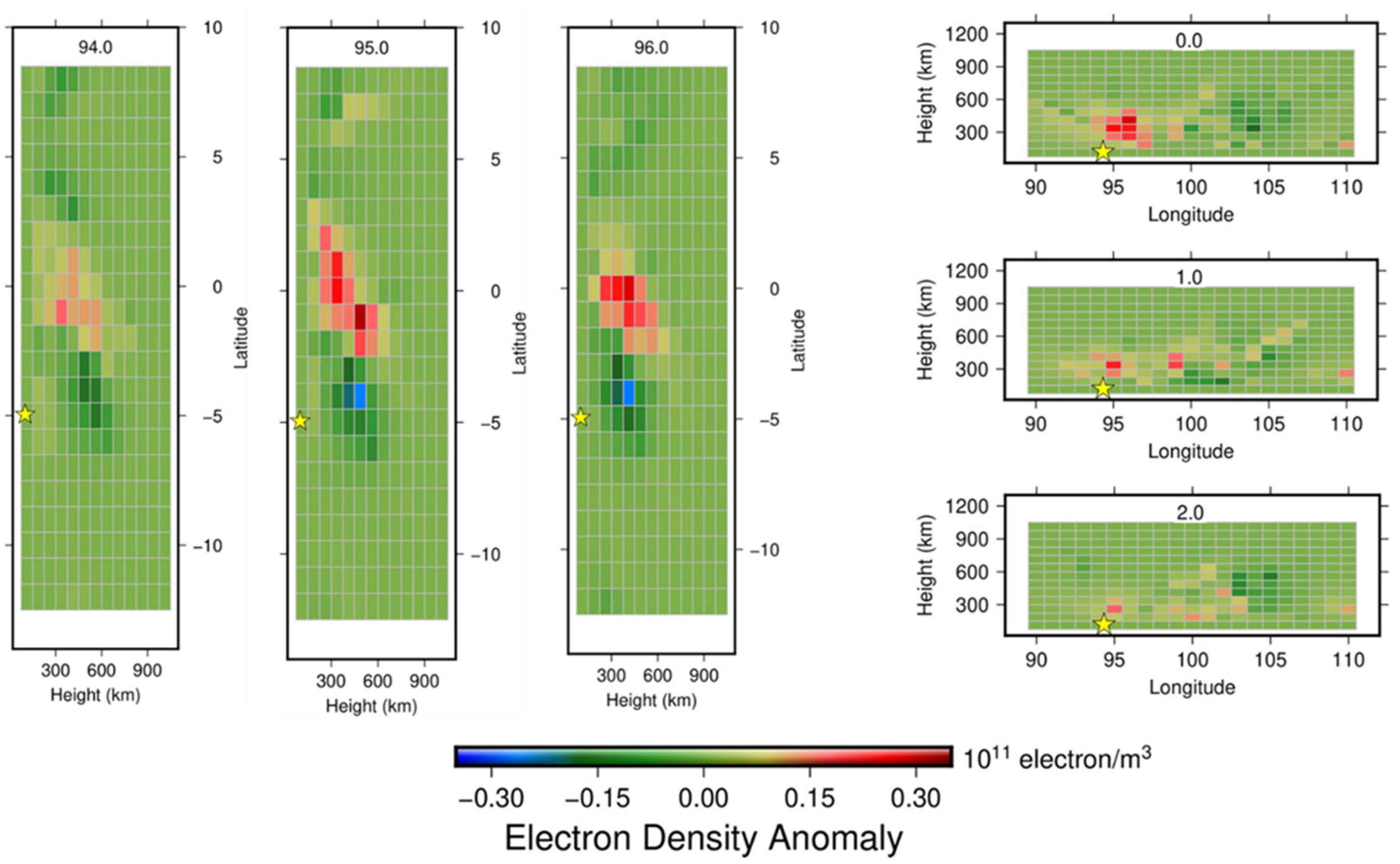
The selected longitudinal profile (longitude: 94°–96° E) and latitude (latitude: 0°–2° S) profile were plotted in
Figure 9 to visualize the vertical structure of the positive and negative anomalies found. The negative anomaly occurs at high latitudes while the positive anomaly is at the low latitude and that anomaly moves toward the geomagnetic field north of the epicenter due to the N-S asymmetry [
14]. The electrons will not move along with neutral particles if the motion of neutral atmospheric particles in the F region is perpendicular to the magnetic field so that the electron density anomaly does not appear. Earthquake epicenters that occurred in the southern hemisphere will cause coseismic ionospheric disturbances that propagate to the north [
1,
5,
15].
This 3D tomography model can be used to observe the movement of anomalies at any time. In this observation carried out in 1-min intervals, as shown in
Figure 8, the movement of the anomaly was analyzed at an altitude of 300 km, where the height is the F2 layer that experienced maximum ionization [
19]. The positive anomaly first appears at 1:02 PM north of the epicenter, moves slowly northward according to the geomagnetic field at ~1–1.62 km s
−1 based on Cahyadi et al. [
5], and decreases every minute before disappearing at 1:11 PM. The movement is also discussed by Cahyadi & Heki [
4] regarding the directivity of the CID based on the geomagnetic field.
Positive and negative anomalies are moving toward the north. Positive anomalies appeared earlier than negative anomalies. The positive and negative anomalies appear at 13:02 UT and 13:04 UT, respectively. This finding is consistent with the N-wave form found in several earthquakes, which started with a positive anomaly and continued with a negative anomaly [
14,
20]. This negative directivity anomaly can be seen clearly at an altitude 400 km (
Figure S2).
The 2016 Sumatra earthquake has a lower angle character between the line-of-sight (LoS) and the CID wavefront so that the detected anomaly begins with a positive signal (positive anomaly). Likewise, the directivity of the acoustic wave moves toward the north. This finding is in accordance with previous research by Heki and Ping [
14]. The focal mechanism of the strike-slip earthquake with a maximum uplift is 1.86 m. An explanation of the CID, directivity, focal mechanism, and the relationship between the moment magnitude and the magnitude of the CID regarding the 2016 Sumatra earthquake in detail is discussed further in Cahyadi et al. [
5].
The magnitude of the earthquake affects the magnitude of the CID because it affects the resulting uplift or subsidence. Processing the Okada [
21] model result, the 2018 Palu earthquake has a strike-slip fault type with an uplift of 1.04 m, as shown in
Figure 5b [
5]. This type of fault has a smaller vertical crustal movement than the dip-slip fault type, so the CID found has a small amplitude consistent with Cahyadi and Heki [
1] ~1/5 of a dip-slip earthquake of the same magnitude. In addition, the epicenter-SIP-receiver geometry relationship also affects the amplitude of CID. This geometric relationship is explained in the observations of Cahyadi and Heki [
1]. The CID observed by this observation dominantly has a good geometric formation: the epicenter-SIP-receiver makes a shallow angle. In addition, the SIP that observed the presence of CID followed the 2016 west Sumatra earthquake, was dominant in the north of the epicenter.
Horizontal Structure & Movement
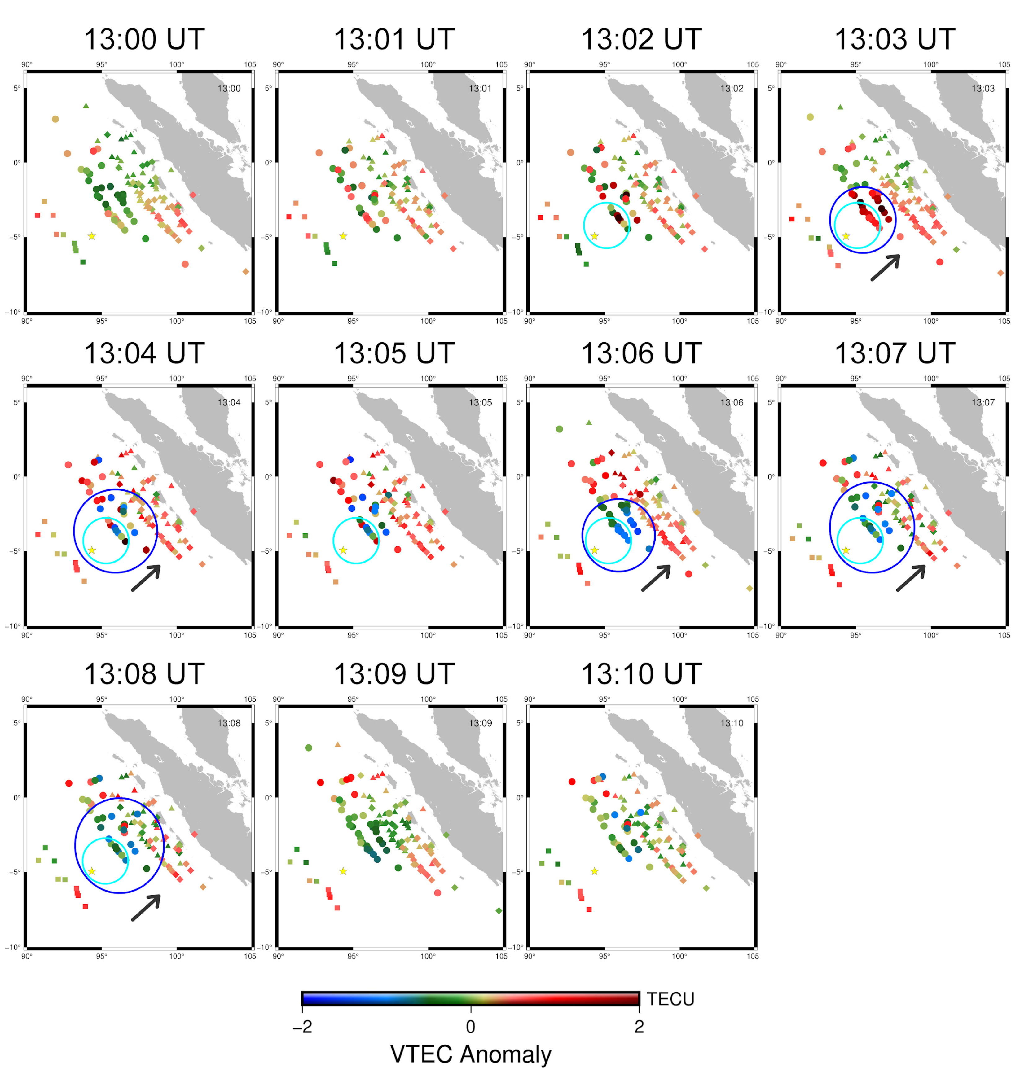
Figure 10 shows the snapshot of VTEC (Vertical Total Electron Content) anomalies at 13:00–13:10 UT around Sumatra drawn with the IPP height of 300 km. The spatial resolution of the VTEC anomaly maps is approximately ~35 km since the distances between INACORS and SUGAR stations are 100 km.
The VTEC anomalies were analyzed on mainshock, at various time epochs (
Figure 8) and studied the time evolution of the horizontal structure. The anomalies are seen at 13:03, 13:04, 13:05, and 13:06 UT. The anomaly is visible at 13:02–13:06 UT. The positive anomaly was seen at 13:02 at coordinates (94° E, −4° N) with a solid color, moving northward, and disappeared at 13:06 UT due to limited SIP observation data. Meanwhile, the negative anomaly appears at 13:05 UT, moves to the north, and disappears 3 min later due to limited SIP observation data and the local nature of CID [
22].
This CID research can be applied as a tsunami early warning system because the tsunami takes more time to reach shores than the acoustic wave reaches the ionospheric F region [
1]. Moreover, Cahyadi et al. [
10] found that the CID of the 2018 Palu Earthquake occurred ~13 min later, followed by a tsunami 20–25 min later. As for earthquake prediction, short-term preseismic anomaly research can only find an increase in ionospheric anomaly phenomena in large earthquakes above Mw8.0 with a duration of ~40 min before the earthquake [
4,
23].


 ,
, 


