Article

Regional Predictions of Air Pollution in Guangzhou: Preliminary Results and Multi-Model Cross-Validations

1
Key Laboratory of Atmospheric Optics, Anhui Institute of Optics and Fine Mechanics, Chinese Academy of Sciences, Hefei 230031, China
2
Advanced Laser Technology Laboratory of Anhui Province, Hefei 230037, China
3
Science Island Branch of Graduate School, University of Science and Technology of China, Hefei 230026, China
4
State Key Laboratory of Organic Geochemistry and Guangdong Key Laboratory of Environmental Protection and Resources Utilization, Guangzhou Institute of Geochemistry, Chinese Academy of Sciences, Guangzhou 510640, China
5
CAS Center for Excellence in Deep Earth Science, Guangzhou 510640, China
6
University of Chinese Academy of Sciences, Beijing 100049, China
7
Guangzhou Sub-Branch of Guangdong Ecological and Environmental Monitoring Center, Guangzhou 510060, China
*
Author to whom correspondence should be addressed.
Atmosphere 2022, 13(10), 1527; https://doi.org/10.3390/atmos13101527
Submission received: 15 August 2022 / Revised: 15 September 2022 / Accepted: 15 September 2022 / Published: 20 September 2022
(This article belongs to the Special Issue Shipping Emissions and Air Pollution)

Abstract

:
A precise air pollution forecast is the basis for targeted pollution control and sustained improvements in air quality. It is desirable and crucial to select the most suitable model for air pollution forecasting (APF). To achieve this goal, this paper provides a comprehensive evaluation of performances of different models in simulating the most common air pollutants (e.g., PM2.5, NO2, SO2, and CO) in Guangzhou (23.13° N, 113.26° E), China. To simulate temporal variations of the above-mentioned air pollutant concentrations in Guangzhou in September and October 2020, we use a numerical forecasting model (i.e., the Weather Research and Forecasting model with Chemistry (WRF-Chem)) and two artificial intelligence models (i.e., the back propagation neural network (BPNN) model and the long short-term memory (LSTM) model). WRF-Chem is also used to simulate the meteorological elements (e.g., the 2 m temperature (T2), 2 m relative humidity (RH), and 10 m wind speed and direction (WS, WD)). In order to investigate the simulation accuracies of classical APF models, we simultaneously compare the simulations of the WRF-Chem, BPNN, and LSTM models to ground truth observations. Comparative assessment results show that WRF-Chem simulated air pollutant (i.e., PM2.5, NO2, SO2, and CO) concentrations have the best correlations with ground measurements (i.e., Pearson correlation coefficient R = 0.88, 0.73, 0.61, and 0.61, respectively). Furthermore, to evaluate model performance in terms of accuracy and stability, the normalized mean bias (NMB, %) and mean fractional bias (MFB, %) are adopted as the standard performance metrics (SPMs) proposed by Boylan et al. The comparison results indicate that when simulating PM2.5, WRF-Chem was more effective than the BPNN but less effective than the LSTM. While simulating concentrations of NO2, SO2, and CO, the WRF-Chem model performed better than the BPNN and LSTM models. With regards to WRF-Chem, the NMBs and MFBs for the PM2.5 simulations are, respectively, 6.49% and 0.02%, –11.96% and –0.031% for NO2, 7.93% and 0.019% for CO, and 5.04% and 0.012% for SO2. Our results suggest that WRF-Chem has superior performance and better accuracy than the NN-based prediction models, making it a promising and useful tool to accurately predict and forecast regional air pollutant concentrations on a city scale.

1. Introduction

Over the past decade, there has been a collective awareness that NO2, SO2, CO, and PM2.5 (atmospheric particle matter with an aerodynamic diameter of ≤ 2.5 μm), as the major substances causing air pollution, have an important effect on climate and human health [1,2,3,4,5,6,7,8,9]. Therefore, China developed a set of National Ambient Air Quality Standards for mitigating air pollution and improving air quality. These emissions reduction policies have had an effective influence on the air quality, significantly reducing the primary air pollutants. In particular, achievements made with respect to air quality improvements in China’s coastal city, Guangzhou, have been good; the daily air quality was up to the secondary standards in 2020 (http://sthjj.gz.gov.cn/zwgk/hjgb/, accessed on: 10/5/2022). A suitable pollutant model can provide optimal simulations of the temporal variations of regional pollutant concentrations; meanwhile, it can help target pollution control and sustain improvements to air quality. Therefore, accurate pollutant models play a crucial role in air pollution control. Previous studies had largely focused on the methods and the use of models for pollutant simulations. However, till now, few studies have been conducted to evaluate different model performances in simulating pollutant concentrations. Thus, it is strongly desired to select the most suitable model for air pollutant studies.
Many operational chemical transport models (CTMs) have been developed for the needs of predicting spatial and temporal air pollutants distributions and providing scientific references for air pollution control and management. The Weather Research and Forecasting model with Chemistry (WRF-Chem), as a typical traditional and continuously updated CTM, has been widely used to handle air pollution problems in different ways [10,11,12,13,14,15]. Grell et al. (2005) proposed WRF-Chem, a WRF model fully coupled online with some chemical mechanisms [16], in which the meteorological and air pollution components use identical time steps, grid resolutions, and transport schemes for all domains. It utilizes state-of-the-art chemical mechanisms and aerosol modules. The WRF-Chem simulations were statistically evaluated based on ground-based observations, firstly, by further comparisons with Mesoscale Model 5-chemistry (MM5-chem) simulations. They reported that the WRF-Chem model performed better in simulating O3 and O3 precursor gas concentrations than the MM5-chem model, but was poorer at simulating other gas-phase species concentrations, due to the use of different planetary boundary layer (PBL) physics parameterization mechanisms. These differences between the two models caused larger biases in the WRF-Chem simulations. However, Grell et al. (2005) did not simulate aerosol concentrations, nor did they evaluate the performance in aerosol simulations [16].
Rocio et al. (2015) assessed the sensitivities of different microphysics schemes used in the WRF-Chem model to simulate aerosol distribution and aerosol–radiation feedback influence [17]. Except for the Morrison and Lin microphysical schemes, two WRF-Chem simulations using the same parameterizations were compared, covering two seasons in 2010. Their comparison results indicated that there were no distinct improvements across the simulations on a large scale using the two selected different microphysical schemes. However, the simulations had different aerosol spatial distributions and statistical pollutant results. Subsequently, Mohan et al. (2018) compared the WRF-Chem simulation performance of different PBL schemes, including the YSU and ACM2 schemes. With observations from four monitoring sites in Delhi, simultaneous comparisons with the two WRF-Chem simulations were conducted to evaluate the model performance for the meteorological elements and pollutant concentrations [18]. Mohan et al. (2018) concluded that the pollutant simulation performance partially depended on the meteorological element conditions. In other words, the PM10 and O3 simulations were good when the wind speed values were smaller than 8 m/s and temperature values were below 40 °C. Furthermore, the ACM2 scheme was found to be the best PBL scheme in Delhi, which improved the WRF-Chem simulation performance for the meteorological and air pollutant variables.
Zhou et al. (2017) applied WRF-Chem to predict PM2.5 concentration over eastern China and showed that it had good correlation with ground measurements and simulation performance [19]. Sha et al. (2019) successfully reproduced four localized haze episodes in Nanjing during two seasons; however, the model performance was poor at the SO2 concentration simulations [20]. To the best of our knowledge, limited studies have utilized high-resolution horizontal grids and emissions inventories to simulate pollutant concentrations. Furthermore, there is a lack of simulations on minimal pollutant concentrations for recent years in Guangzhou. Most previous studies have solely used the WRF-Chem model and evaluated the simulation accuracy and performance against ground observations. Some studies have compared the simulated accuracy of different air quality models [21,22,23,24]. Zhang et al. (2016) compared WRF-Chem with the Community Multiscale Air Quality (CMAQ) model for meteorological and pollutant simulation performance over East Asia [25]. They showed that CMAQ yielded better simulations than those of the WRF-Chem model for meteorological elements. However, they did not meticulously consider the specific pollutant simulation differences between these models.
An increasing number of studies have used different neural network (NN) models to simulate pollutant concentrations, with evaluations on the precision and performance of those models [26,27,28,29,30]. Ni et al. (2018) used the meteorological and satellite-derived aerosol optical depth (AOD) to simulate the PM2.5 concentrations. They simulated PM2.5 variability and diurnal variations in the Beijing–Tianjin–Hebei (BTH) region using the BPNN model, finding that the BPNN simulations showed a similar yearly variation in comparison with ground observations [31]. The results showed that the PM2.5 concentrations estimated from the BPNN model have good correlations with the observed PM2.5 concentrations (R2 = 0.68). Meanwhile, although they found that the 10-fold cross-validation method overestimates the concentrations, the simulated result closely estimated the observed concentrations (R2 = 0.54). The BPNN model was nevertheless not compared with other NN models in their study.
Li et al. (2017) proposed a long short-term memory neural network extended model (LSTME) to simulate the pollutant concentrations [32]. They extracted the features from the historical pollutant concentrations and meteorological elements for predicting the future pollutant concentrations. The prediction results of the LSTME model were verified by the observed concentrations; meanwhile, they found that the LSTME model performed well, with a root mean square error (RMSE) of 41.94% and a mean absolute percentage error (MAPE) of 31.47%. In addition, the LSTME model was compared with several other NN models, as indicated by the spatiotemporal deep learning model, the time delay NN model, the support vector regression model, etc. The study showed that the LSTME model performance was superior to the other NN models’ performances based on criteria such as RMSE, MAPE, and mean absolute error (MAE). However, they did not evaluate the trend of simulating temporal variations and the correlation coefficient with the observed data.
All things considered, these studies focused on the single model simulation performance, or the comparisons between different CTMs or NN models. Recent comprehensive evaluations of the accuracy and performance of air pollutant simulations between CTM and NN models, as well as discussions on their discrepancies over Guangzhou, remain scarce.
The CTMs simply and reasonably expressed the atmospheric movement and the reaction of air pollutants by the parameterization schemes, so they can explain the causes of simulation errors by the physical mechanism and the meteorological conditions, but they needed the initial and boundary conditions, emissions inventories, and substantial computational resources. As one of the CTMs, WRF-Chem has been continually optimizing, and the improved parameterization schemes can simply and reasonably express the atmospheric movement and the reaction of air pollutants. Meanwhile, previous studies showed that the WRF-Chem model has superior performance in simulating the pollutant concentrations and is widely used [10,11,12,13,14,15,16,17,18,19,20,21,22,23,24]. Thus, for the CTM, we chose the WRF-Chem model in this study.
With the growth in big data analytics and artificial intelligence, the use of NN models had received international attention and more and more countries were conducting research in this field. The growth has provided the meteorological and environmental communities with constantly enlarging resources for data acquisition. Nowadays, many data-driven models, especially NN models, had been widely used to handle meteorological and environmental problems in different ways [26,27,28,29,30,31,32]. Although NN models did not have any physical meaning, and the model performance and simulation results were closely linked to the types of input data and the amount of training data, they predicated pollutant concentrations by training NN models using the historical meteorological elements and pollutant concentrations, so the substantial computational resources and boundary conditions were not necessarily needed. The BPNN model, proposed by Rumelhart et al. [33], was one of the most widely use artificial neural network (ANN) models. In the BPNN model, the entire arithmetic process consisted of two parts: forward propagation and error back propagation, and one can obtain satisfactory simulation results due to the reasonable arithmetic structures. The LSTM model was an extension of the recurrent neural network (RNN) models, and it can solve the exploding and vanishing gradient problem, which inhibited the simulation precision for previous RNN models. In recent years, many studies showed that the LSTM model had good results in time series simulations under specific conditions [34,35,36,37]. Meanwhile, the BPNN and LSTM models had superior performance in simulating the pollutant concentrations (Table 1). In this study, we chose the BPNN and LSTM models to conduct model cross-validations between them both and WRF-Chem.
In this paper, the WRF-Chem model, using updated emissions inventory with finer horizontal resolution, was employed to predict the pollutant concentrations in Guangzhou. In view of the fact that the NN models had superior performances in simulating the pollutant concentrations, we also constructed the frequently used NN models to predict air pollution in Guangzhou. By comparing WRF-Chem to ground observations and the NN models, the most suitable pollutant model was then proposed. To evaluate the performance of the WRF-Chem and NN models, standard model performance metrics were adopted. Preliminary results were presented and analyzed in Section 3 followed by discussion in Section 4. The final section contains conclusions on the performances of the WRF-Chem and the NN models in the air pollutant concentrations forecasting.

2. Methods, Data, and Model Simulation Evaluation

2.1. Model Descriptions

2.1.1. WRF-Chem Model Configuration

The WRF-Chem model was developed by NCAR, the Pacific Northwest National Laboratory (PNNL) and the National Oceanic and Atmospheric Administration (NOAA). It consists of an online model that can simulate meteorological data, together with the emissions, transport, diffusion, and deposition of pollutants [14]. Therefore, we used WRF-Chem version 4.3 to simulate the meteorological elements and pollutant concentrations of Guangzhou. The simulation period was from 11 September to 7 October 2020. The initial conditions had a non-negligible interference on the simulation accuracies and performances of the WRF-Chem model at the beginning of the simulation, so we needed a spin-up period to minimize interference from the initial conditions. In this study, the first 10 d was treated as a spin-up period and were not used to evaluate the simulation performance. Three nested domains were selected to obtain more precise simulation results for Guangzhou. The innermost domain (d03) had a finer spatial resolution of 3 km × 3 km, covering the entirety of Guangzhou City and most parts of Guangdong Province, as denoted by the red line in Figure 1. The second domain (d02) contained the innermost domain covering most of southern China on a 9 km × 9 km grid. The two domains were encompassed by a larger domain with a spatial resolution of 27 km × 27 km, which covered most of China, as depicted in Figure 1, to realize air pollution exchange. The time steps of the model were set to 180, 60, and 20 s for the three domains, respectively. Each domain was divided into 35 vertical levels; the top of the model was set at 50 hPa. Table 2 lists the details of the key parameterization schemes. The Carbon Bond Mechanism Z (CBMZ) [38] gas-phase chemistry mechanism and 4-bin MOSAIC [39] aerosol model were selected for this study.
For the initial and boundary conditions, the meteorological data were derived from the National Center for Environmental Prediction (NCEP) Final Analysis 6-hourly dataset (http://rda.ucar.edu/datasets/ds083.2/, accessed on: 10/5/2022), with a spatial resolution of 1° × 1°, which is updated every 6 h. Meanwhile, we used NCEP Automatic Data Processing (ADP) Global Upper Air Observational Weather Data (http://rda.ucar.edu/datasets/ds351.0/, accessed on: 10/5/2022) and Global Surface Observational Weather Data (http://rda.ucar.edu/datasets/ds461.0/, accessed on: 10/5/2022) to perform simulation nudging (using a coefficient of 0.0003 s–1). We also updated the sea surface temperature (SST) using the TAVGSFC program.
For the inventory emissions, the anthropogenic emissions were based on the Multi-resolution Emission Inventory for China (MEIC, 2017: http://www.meicmodel.org, accessed on: 10/5/2022). In this study, the outermost domain had the same spatial resolution with the MEIC. Unfortunately, we did not have all the actual emissions data in China in 2020; meanwhile, the inventory emission for the outermost domain had little influence on the pollutant simulation accuracy in the innermost domain. Therefore, we used the MEIC directly as the inventory emission for the outermost domain [48,49]. However, the highest spatial resolution of MEIC was only 27 km, and it cannot meet the simulation needs of the WRF-Chem model. Therefore, we used the NCAR Command Language (NCL) to structure the framework for the inner inventory emissions, which had the same grid amount and geographic information (i.e., longitude, latitude, terrain height, spatial resolution, etc.) with the input meteorological data. We then spatially allocated the MEIC emissions data into the framework based on the population density (https://hub.worldpop.org/geodata/listing?id=77, accessed on: 10/5/2022), so that we could obtain higher resolution (i.e., 9 km × 9 km (d02), 3 km × 3 km (d03)) inventory emissions. Meanwhile, there were obvious differences in the pollutant concentrations in Guangzhou between 2017 and 2020 (Figure 2), so the inner emissions inventories of 2017 were not applicable for simulating the pollutant concentrations of 2020. Considering those differences, we adapted the inner-domain inventory emissions to more optimally match the simulation according to the numerical differences in the pollutant concentrations between 2017 and 2020. We obtained the modified inventory emissions by multiplying the emission rate of 2017 with the ratios of the pollutant concentrations in 2017 and 2020. Like the MEIC, the updated emissions inventories were the bottom-up emissions inventories frameworks. Part of the final inner-domains emissions inventories are depicted in Figure 3.

2.1.2. Back Propagation Neural Network

We constructed a conventional back propagation neural network (BPNN) as a simulation model with three layers (i.e., the input, the hidden, and the output layers), which acted as a universal function approximator (UFA) [50,51,52]. Thus, the model had the desired properties and yielded reliable baseline results. The BPNN model belonged to the ANN model and the entire arithmetic process consisted of two parts: forward propagation and error back propagation. Figure 4a shows a schematic of the BPNN. During the forward propagation process, we fed the hourly observations into the input layer. The input information then passed through the input and hidden layers to the output layer. Finally, we obtained the simulation results. If the expected simulation results could not be obtained from the output layer, we used arithmetic to perform error back propagation. Error back propagation used the decreasing gradient algorithm; therefore, we more rapidly obtained the minimum of the function in the opposite direction. During this process, the expected error was regarded as the objective function. The weight was modified according to the gradient; NN learning was completed during the weight modification process. BPNN learning did not end until the error conformed to pre-determined expectations. The detailed structure of the BPNN model was depicted in Figure 4b, with black lines representing the nonlinear activation functions and the optimized weights in the BPNN model learning process. The complex combination of the nonlinear activation functions and weights made the model feasible to simulate the pollutant concentrations.
In this study, 5-fold cross-validation was applied to the entire dataset, which was divided into a training dataset (i.e., 672 data samples or 80%) and a testing dataset (i.e., 168 data samples or 20%). For the input layer (Figure 4b), we fed the hourly meteorological data (i.e., the 2 m temperature T2, 2 m relative humidity RH, 10 m wind speed WS, and 10 m wind direction WD). The selection of the number of nodes was important in the hidden layer. Studies have shown that the approximate limit of the number of nodes for the majority of applications ranges from 2√X + 1 to 2X + Y, where X and Y are the number of nodes in the input and output layers, respectively [53,54]. With four inputs from the observations and a single output, we obtained the optimal number of nodes in the hidden layer of the BPNN, ranging from 5 to 9, via continuous simulations. Although the BPNN architecture proposed in this study only had a single linear output node, we could simulate different pollutant concentrations by changing the output results, such as PM2.5, NO2, CO, and SO2.

2.1.3. Long Short-Term Memory

As previously discussed, the RNN models may be inhibited owing to the learning of long-term dependencies. The LSTM model, as an extension of the RNN, can solve the exploding and vanishing gradient problem using a great method [55,56,57]. The LSTM model cells were used to independently learn the inherent useful characteristics from the previous observed pollutant concentrations, while ancillary data, including time stamp data and meteorological elements, were combined with the LSTM model to improve the model performance (Figure 5a). Thus, the historical meteorological elements and pollutant concentrations influence the current pollutant concentrations. In this study, we constructed a unique LSTM to extract the characteristics of the time series which could predict the pollutant concentrations. Meanwhile, we preset several parameters before constructing the LSTM model, including the quantity of the LSTM layers, the quantity of the fully connected layers, the learning rate, etc. Finally, the LSTM model can predict the pollutant concentrations in the following several hours by learning the previous diurnal variabilities in these pollutant concentrations and meteorological elements, which were input into the LSTM. Similar to the data division and cross-validation for the BPNN, the dataset was divided into 80% of the samples as the training set and 20% of the samples as the test set.
Additionally, Figure 5b shows the cell structure of an LSTM. The LSTM model contained many LSTM cells; each cell comprised three multiplicative gates (i.e., an input gate, a forget gate, and an output gate). First, the historical meteorological elements and pollutant concentrations were entered into the model spatial combinatory through the input gate; therefore, the input gate controlled the observation’s influence on the simulation. The information then forgot some previous concentration data factors to control and protect information transmission in the forget gate. The sigmoid and “tanh” layers determined whether the information was to accumulate in the unit state, while the “tanh” layer invented a new value vector to update the state of the cell [57]. After the cell gate update, the output and cell gates decided the output information, because the output and cell gates controlled the influence of the historical trends. For instance, the output and cell gates trended to off to maintain the trend information when the pollutant concentrations changed slightly. Ultimately, we obtained the simulated results from the LSTM model, i.e., PM2.5, NO2, CO, and SO2 concentrations.

2.2. Observed Data

The meteorological and pollutant data used in this study were obtained from the Guangzhou Environmental Monitoring Centre. The data were measured at the Guangzhou downtown superstation (see the red dot in Figure 1) that was located in the center of Guangzhou, so the observed pollutants belonged to urban pollution. During actual conditions, there were some errors in the measurement instruments or due to human factors which may have led to outliers or NaN (not a value) in the observations. Therefore, the original observations collected were pre-processed and cleaned. We replaced outliers with NaN; if there were ≥3 consecutive NaN terms, we deleted the observations for this period. Otherwise, NaN was replaced via linear interpolation. Finally, the observed data from the monitoring station were compared with the simulated results of the nearest model grid and NN. The comparative data contained T2, RH, WS, WD and PM2.5, NO2, CO, and SO2 concentrations. Meanwhile, Table 3 presents the features contained in the comparative data.

2.3. Model Simulation Evaluation

We simultaneously evaluated the meteorological elements with respect to the ground observations. The evaluation parameters included the mean bias (MB), mean error (ME), standard deviation (SD), root mean square error (RMSE), and the Pearson correlation coefficient (CC) R [58]. However, for pollutant concentrations, we used other standard performance parameters, including the normalized mean bias (NMB), mean fractional bias (MFB) [59], and quantile–quantile (Q–Q) plots. These evaluation parameters were used to evaluate the simulation accuracies and the performances of the proposed models from different sides:
(1)
MB and ME are, respectively, the average and absolute error between the simulated results (Cm) and the observed results (Co). They can show actual situations of the simulated value errors. RMSE is the arithmetic square root of the mean square error (MSE), while the MSE is the average value of the square of the error between the simulated results (Cm) and the observed results (Co). The smaller the values of MB, ME, and RMSE, the better the accuracy of the model simulated result.
(2)
To evaluate the simulation ability of the models, we choose the Pearson CC to measure how well the simulated results fit the observed results. The larger the CC value, the better the regression effect and the more accurate the model. If the value of R is more than 0.6, we think the model has good accuracy.
(3)
NMB or (and) MFB can provide a good sense of the model performance, in that it does not need an observation-based minimum threshold. The NMB ranges from −100% to +∞ while MFB from −200% to +200%. These indices have the advantage of limiting the maximum deviation; meanwhile, they are widely used for evaluating the model performance in the accuracy of the pollutant concentration simulations. The model performance has met the criteria when the MFB is less than or equal to ± 60% [59]. In this study, the model is regarded as having superior model performance when the MFB is <± 45%.
Details of standard performance metrics and criteria are listed in Table 4.

3. Results

3.1. Meteorological Element Evaluation

As shown in Figure 6, the hourly variations in the WRF-Chem simulations were compared with the observed data for the meteorological elements, which contained the T2, RH, WS, and WD in Guangzhou. The WRF-Chem model effectively captured the temporal variations and the peaks of the meteorological elements. During the simulation, the correlations for T2, RH, and WS were 0.95, 0.88, and 0.64, respectively. The simulated meteorological elements were all higher than the observations, while the MB values were all less than 0.24 ℃, 3.57%, and 0.37 m/s, respectively, as listed in Table 5 and shown in Figure 7.

3.2. Pollutant Concentration Evaluation

Figure 8 compares the temporal variations in the observed and simulated PM2.5, NO2, SO2, and CO concentrations in Guangzhou during the study period. Table 6 lists the NMB, MFB, and R achieved by each model when simulating the different pollutant concentrations. For the PM2.5 concentration, there was a significant correlation between the WRF-Chem simulated PM2.5 and the observed concentrations (R = 0.80). Meanwhile, we compared the WRF-Chem model with different NN models, i.e., the BPNN and the LSTM. As listed in Table 6 and shown in Figure 8 and Figure 9, we found that the BPNN model cannot efficiently capture the PM2.5 concentration trends as well as peaks and had a poor correlation with the observed concentration (R = 0.33). The LSTM model simulation reflects the PM2.5 temporal variation better than other model simulations and it had the best correlation with the observed concentration (R = 0.85). Figure 10 shows the MFB for each hourly simulated concentration. The black solid lines represent the MFB evaluation criteria, which was raised by Boylan et al. (2006) to evaluate model performance in terms of accuracy and stability. Meanwhile, to compare further and choose the most suitable pollutant model, the blue-dashed lines represent our proposed objective for the MFB (45%). When the circles fall inside the blue-dashed lines, the model is regarded as having superior model performance for the pollutant concentration simulation at this time. As shown in Figure 10a, the performance of the WRF-Chem model at simulating the PM2.5 concentration levels was optimal. The WRF-Chem simulation conformed to the MFB criteria < ±60% of the study period, while the whole simulated results achieved our proposed objective for the MFB (45%). For the NN models, the BPNN simulation cannot meet our proposed objective for the MFB, while most of the LSTM simulated results can. Additionally, Figure 11 shows the different model performances in the Taylor diagrams, which were also often used to evaluate the simulation accuracies. In the Taylor diagram, different colored circles represent different models. The correlation coefficients were determined by azimuth positions of the models, with the closer the circle is to the x-axis, the higher correlation the model has with the observations. The radial distance from the circles represents the SD of the model simulations, indicating the model’s ability to simulate center amplitude. Meanwhile, the RMSE is indicated by the distance between the different circles and the black dot (the observation). As shown in Figure 11a, the WRF-Chem correlation coefficient and simulation accuracy were slightly worse than those of the LSTM model, but the WRF-Chem model significantly outperformed the BPNN model.
Compared with the observed NO2 concentration, although the BPNN model simulations conformed to the standards of the USEPA, with an NMB of −7.16% and an MFB of 0.018% according to Table 6 and Figure 10, the model did not reflect the temporal variation and captured the NO2 concentrations peak (Figure 8 and Figure 9). Moreover, the correlation between the BPNN model simulated NO2 concentrations and the observed concentrations was undesired (R = 0.55). The LSTM model captured the temporal variations better than other models and conformed to the standards of the USEPA, with an NMB of 7.95% and an MFB of 0.019%, but the correlation coefficient (R = 0.68) was worse than the WRF-Chem model (R = 0.73) (Figure 11b). For the WRF-Chem model, although some simulated results cannot achieve our proposed objective for the MFB, the whole simulated results conformed to the MFB criteria < ±60% (Figure 10); meanwhile, it still effectively simulated the temporal variation in the NO2 concentrations and the distribution of the extreme values (Figure 8 and Figure 9). In addition, the Taylor diagram for NO2 in Figure 11b demonstrated the performance of the different models. For all models’ simulations (CTM and NN models), the highest correlation coefficient, SD, and RMSE were observed for WRF-Chem.
Figure 8 shows a comparison of the SO2 concentration time series between the observations and model simulations. The WRF-Chem and LSTM model simulations were superior to that of the BPNN model. The magnitudes of the simulated SO2 concentrations by these two models were approximately consistent with the observations (Figure 9). WRF-Chem captured the SO2 concentration trends and outperformed the LSTM model, despite agreements in the simulation error and performance gap between the two models (NMBs of 5.04 and −10.49%, respectively; MFBs of 0.012 and −0.026%, respectively), as shown in Table 6 and Figure 9 and Figure 10. The Taylor diagram for SO2 in Figure 11c shows that the BPNN model yielded the minimum R value (R = 0.38), while the correlation coefficient for the LSTM (R = 0.60) was slightly inferior to that of WRF-Chem (R = 0.61). Meanwhile, the SD and RMSE of the WRF-Chem model were obviously better than those of the NN models. The overall situation for CO was largely identical to that of SO2, i.e., the model simulation error and performance, and sequence of correlation coefficients for each model.

4. Discussion

For the simulation of meteorological elements, model evaluations indicated that the meteorological elements with simulation nudging were reasonable for Guangzhou (Figure 6). However, we found that the 10 m wind speed did not obviously improve compared with the other meteorological simulations (Table 6). This phenomenon is caused by the presence of numerous buildings adjacent to the monitoring site. In addition, the air pollution simulation accuracy was closely related to the meteorological element simulation accuracy. On the one hand, the overestimated WS may have caused biases in the pollutant concentrations; on the other hand, the overestimated T2 and RH may have led to biases in the temperature or relative humidity-dependent reaction factors in the WRF-Chem simulation. Overall, the WRF-Chem model had an excellent performance on the meteorological element simulation in Guangzhou.
For the PM2.5 concentration simulation, the trend and magnitude produced by the WRF-Chem simulation using the new emissions inventory were consistent with the ground observations. Temporally, there were some underestimations from 25 to 26 September and 4 to 6 October, with an increasing trend observed from 1 to 2 October; however, WRF-Chem efficiently captured the other peaks, which appeared on September 21 to 24 and 27 to 30 and other days. There was therefore a significant correlation between the WRF-Chem simulated PM2.5 concentration and the observed concentration (R = 0.80). Although there were some underestimation and overestimation between the WRF-Chem simulated and the observed PM2.5 concentrations, the relative errors were small. Thus, the whole simulated PM2.5 concentration achieved our proposed objective for the MFB. In the BPNN model, the model generally underestimated PM
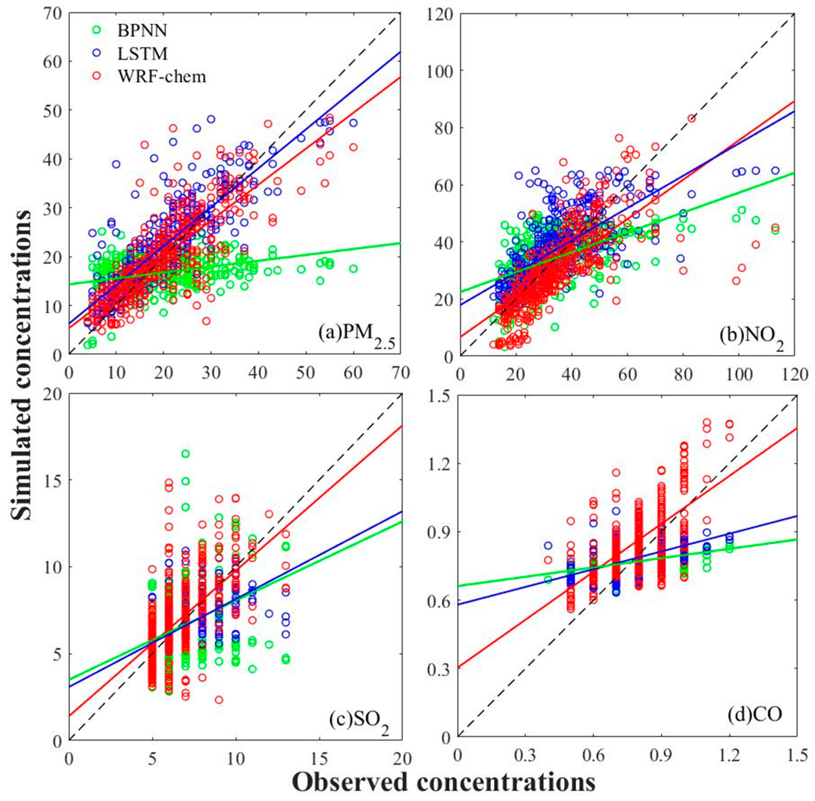
2.5 concentration and inefficiently captured the peaks. Meanwhile, the generally larger errors that led to the BPNN simulation cannot meet our proposed objective for the MFB. In addition, we found that the LSTM simulation has suboptimal MFB results in a few time periods, though the LSTM simulation had the best correlation with the observations; moreover, the LSTM could not capture the peak of the observed concentration, as compared to that of WRF-Chem, as shown in Figure 8. To sum up, the WRF-Chem simulation was more reasonable and superior to the BPNN model, but slightly worse than the LSTM in terms of the simulation trend, errors, and correlation coefficient (c.f., Figure 8, Figure 10 and Figure 11). The results may be caused by several factors. First, there were some deviations between the WRF-Chem meteorological simulations and the observations, such as the overestimated WS, T2, and RH. The air pollution concentrations were closely related to the meteorological elements. For example, the WS had a direct influence on the dilution and diffusion of the aerosol [60], and the other meteorological elements also affected the pollutant concentrations through the wind. The overestimated wind speed can cause an underestimated PM2.5 concentration by the WRF-Chem model. Therefore, the meteorological simulation errors of the WRF-Chem model led to simulation pollutant concentration errors. Second, the emissions inventory provided initial conditions and emissions data of the air pollutants for the WRF-Chem model. Meanwhile, Li et al. (2017) verified that there were some differences in the simulations of different emissions inventories, and they emphasized that the low resolution and large uncertainty of the emissions inventory produce large simulation errors [61]. In this study, the WRF-Chem emissions inventory was modified by the monthly emissions data, which were provided by the Guangzhou Environmental Monitoring Centre, and the frequency of the modification was one month. Unfortunately, we cannot obtain the actual spatial distributions of the daily and hourly emissions data to modify the emissions inventory more accurately, so that partial nondeterminacy exists in the new emissions inventory [62]. Ultimately, the nondeterminacy caused the simulation errors in the WRF-Chem model. Third, the BPNN algorithms are used as a black-box so that we cannot clearly explain how the BPNN model estimates the pollutant concentrations. Meanwhile, the approximation and generalization abilities of the NN models were closely related to the input data [63]. There were few types of input data and a small amount of training data for the BPNN model in this study, so the BPNN model simulation was not satisfactory. Finally, unlike the traditional RNNs, the LSTM model is capable of learning the long time series, and it can effectively and automatically extract the temporal correlation within the pollutant concentrations. Meanwhile, the LSTM model was not influenced by the vanishing gradient problem. These features were extremely important for simulating the precise temporal pollutant processes. Therefore, the LSTM model can accurately simulate the pollutant concentrations with the obvious change characteristics of a time series. Moreover, using the auxiliary data (i.e., T2, RH, WS, and WD) can enhance the simulation performances in the LSTM model [32]. The PM2.5 concentrations were greatly increased and the change was evident during this observation period, so the LSTM model captured the temporal variations well. In total, WRF-Chem simulated PM2.5 concentration, more reasonably reflected hourly variability, and actually captured peaks of the observations.
For the NO2 concentration simulation, the WRF-Chem model underestimated the NO2 concentrations from 5 to 7 October, and this finally caused some simulated concentrations that cannot achieve our proposed objective for the MFB. During this period, the emissions inventory was less accurate for NO2 concentration simulation; moreover, the WRF-Chem simulated high wind speeds may account for the NO2 concentration underestimation. However, in general, the WRF-Chem model simulated the trend and magnitude well. In terms of the NO2 concentration simulations, the WRF-Chem model significantly outperformed the LSTM and BPNN models, and had a large advantage with an accurate simulation. For the SO2 and CO concentration simulations, we filter the observed data, i.e., if more than 25% of the observed values were below the detection limit, we cannot account for these data in our study. We found that both types of air pollutants met the data demand. By comparing the different models’ simulated results, the WRF-Chem model was superior to the LSTM and BPNN models in the simulated trend, error, performance, etc. In addition, the BPNN model cannot yet capture the SO2 and CO concentration temporal variations, although the whole simulated results achieved our proposed objective for the MFB. Meanwhile, the CCs for SO2 (R = 0.60) and CO (R = 0.50) were slightly inferior to those of other air pollutants by the LSTM. Several factors accounted for these phenomena. First, the WRF-Chem meteorological simulation errors and partial nondeterminacy of the emissions inventory were not ignorable, as stated earlier. Second, previous studies showed that the microphysics and CBMZ gas-phase chemistry mechanisms in the WRF-Chem model need to be further improved for better simulations [20,64]. For the microphysics mechanism, there were lower cloud fractions and liquid water path in the WRF-Chem model, which could result in the weak in-cloud sulfate and the lower sulfate mass. For the chemical mechanism, the CBMZ gas-phase chemistry mechanism had produced an incorrect conversion rate for SO2 to sulfate; meanwhile, the mechanism did not consider the parameters on the heterogeneous reaction rate. These limitations ultimately led to the simulation bias for SO2 in WRF-Chem. Third, the precision of the observation instrument for the SO2 and CO concentrations was significantly smaller than those of the models’ simulations; therefore, the observations could not reflect subtle changes in the trend, which existed in the model simulation. Finally, the SO2 and CO concentration time series had no obvious regularities. As mentioned above, the LSTM cannot effectively simulate variables without temporal regularity; hence, the LSTM led to inaccurate simulations. In summary, WRF-Chem was superior to the LSTM and BPNN models for simulating SO2 and CO concentrations.
All things considered, the WRF-Chem model can accurately predict all the air pollutant concentrations and reasonably capture their diurnal variability after mitigating air pollution. Meanwhile, it was the most suitable pollutant model in Guangzhou, because the WRF-Chem model had a superior model performance and better simulated results than the NN models. Furthermore, WRF-Chem can provide source apportionment, transboundary transport, and backward trajectories for different pollutants in future studies, which is not possible with the LSTM and BPNN models.

5. Conclusions

Selecting an appropriate model to precisely predict pollutant concentrations remains a challenge in pollution control and environmental management. This study focused on the performance of the WRF-Chem model in simulating the PM2.5, NO2, SO2, and CO concentrations in Guangzhou. We also performed comparisons to evaluate the differences between the WRF-Chem and NN models with respect to the observed concentrations. The main findings of this study are summarized as follows:
(1)
Compared with the monitoring station observations, WRF-Chem can reasonably simulate the magnitude and temporal variations in the air pollutant concentrations, capture the peaks of the observed concentrations, and conform to the evaluation criterion for model performance.
(2)
For the PM2.5 concentration simulations, WRF-Chem was superior to the BPNN model in all respects such as simulation bias, correlation coefficient, and model performance. Although the WRF-Chem correlation coefficient and model performance were slightly worse than those of the LSTM, WRF-Chem more effectively simulated the extremum than the LSTM. For the other pollutant concentrations, the WRF-Chem model correlation coefficients and model performances were better than those of the LSTM and BPNN. According to the negligible simulation error, excellent simulation performance, and high correlation, the WRF-Chem simulation was superior and the most reasonable for all pollutants.
(3)
As model input data, the observed pollutant concentrations were directly related to the NN model simulated results. In other words, the types and amounts of input data had a crucial influence on the simulation accuracies and performances of the NN models, especially for the BPNN model. If there are enough types and amounts of input data, the BPNN model can use the gradient search technique to minimize the MSE between the output data and testing data. In this case, the BPNN model can accurately simulate the pollutant concentrations. The LSTM model simulated the pollutant concentrations by effectively and automatically extracting the temporal correlations within the previous concentrations (the input data), so they also influenced the LSTM model performance. The LSTM model can capture the pollutant concentrations and have considerable model performance, on condition that the pollutant concentration time series had obvious regularities. However, insufficient types and amounts of input data, and the limited accuracies of the SO2 and CO measuring apparatuses, ultimately resulted in relatively poor NN models’ performance.
(4)
The meteorological input data, which served as the initial and boundary meteorological conditions for the WRF-Chem model, were indispensable. Meanwhile, the meteorological input data helped us obtain precise meteorological element simulations, and ultimately enhance the simulation accuracy of the pollutant concentration. As emission input data, the emissions inventories directly provide the emissions data (i.e., the emission rate and the emission allocation) to the WRF-Chem model, so the modified emissions inventories can contribute largely and positively to accurate pollutant concentration simulations in the study.
In summary, this suggests several important points: (1) the emissions inventory revision time interval should be more accurate; (2) the NO2, SO2, and CO emissions were imprecise in the new emissions inventory; (3) the parameterization schemes and gas-phase chemistry mechanism need further improvement for better simulating the SO2 and CO concentrations; (4) the BPNN model needs more types of input data to improve the pollutant concentration simulation accuracy; and (5) the SO2 and CO observed concentration time series had no obvious regularities, so the LSTM model cannot capture the concentration temporal variation.
Generally, the WRF-Chem model had a significant positive influence on the simulated pollutant concentrations in Guangzhou. We suggest using the WRF-Chem model to simulate the PM2.5 and NO2 concentrations owing to its precise and reasonable simulations, as well as the presence of several improvements in the simulations compared with the BPNN and LSTM models. Additionally, the WRF-Chem simulated SO2 and CO concentrations were broadly similar to the observations, but there were some differences which require more accurate daily or hourly emissions data. Therefore, building hourly emissions inventories requires a higher spatial resolution, up-to-date provincial emissions data, and extra monitoring data. The application of accurate daily or hourly emissions can provide improvements in the WRF-Chem simulation compared with NN models.

Author Contributions

Conceptualization, Z.Q., S.C., and X.W.; design, Z.Q., S.C. and X.W.; data collection, Z.Q., Z.Y., C.P., L.L. and Z.Z.; data analysis, Z.Q., Z.Y., C.P., L.L. and Z.Z.; writing—original draft preparation, Z.Q. and S.C.; funding, T.L., S.C., X.L., and W.Z. All authors have read and agreed to the published version of the manuscript.

Funding

This research was supported by the Foundation of Key Laboratory of Science and the Technology Innovation of the Chinese Academy of Sciences (CXJJ-21S028), and the Strategic Priority Research Program of the Chinese Academy of Sciences (XDA17010104).

Data Availability Statement

The Final Analysis 6-hourly datasets are available at http://rda.ucar.edu/datasets/ds083.2/, accessed on: 10/5/2022. The NCEP ADP Global Upper Air Observational Weather Data are available at http://rda.ucar.edu/datasets/ds351.0/, accessed on: 10/5/2022. The NCEP ADP Global Surface Observational Weather Data are available at http://rda.ucar.edu/datasets/ds461.0/, accessed on: 10/5/2022.

Acknowledgments

The authors thank Guangzhou Environmental Monitoring Center for offering the observed data over Guangzhou.

Conflicts of Interest

The authors declare no conflict of interest.

Abbreviations

air pollution forecasting (APF); Weather Research and Forecasting model with Chemistry (WRF-Chem); 2 m temperature (T2); 2 m relative humidity (RH); normalized mean bias (NMB); mean fractional bias (MFB); U.S. Environmental Protection Agency (USEPA); Community Multiscale Air Quality (CMAQ); neural network (NN); back propagation neural network (BPNN); long short-term memory (LSTM); atmospheric particle matter with an aerodynamic diameter of ≤2.5 μm (PM2.5); chemical transport model (CTM); Mesoscale Model 5-chemistry (MM5-chem); planetary boundary layer (PBL); aerosol optical depth (AOD); Beijing–Tianjin–Hebei (BTH); long short-term memory neural network extended model (LSTME); root mean square error (RMSE); mean absolute percentage error (MAPE); mean absolute error (MAE); Pacific Northwest National Laboratory (PNNL); National Oceanic and Atmospheric Administration (NOAA); Carbon Bond Mechanism Z (CBMZ); National Center for Environmental Prediction (NCEP); the NCAR Command Language (NCL); automatic data processing (ADP); sea surface temperature (SST); universal function approximator (UFA); artificial neural network (ANN); 10 m wind speed (WS); 10 m wind direction (WD); recurrent neural network (RNN); mean bias (MB); mean error (ME); standard deviation (SD); correlation coefficient (CC); quantile–quantile (Q–Q); mean square error (MSE).

References

  1. Hyslop, N.P. Impaired visibility: The air pollution people see. Atmos. Environ. 2009, 43, 182–195. [Google Scholar] [CrossRef]
  2. Akimoto, H. Global air quality and pollution. Science 2003, 302, 1716–1719. [Google Scholar] [CrossRef] [PubMed]
  3. Lelieveld, J.; Evans, J.S.; Fnais, M.; Giannadaki, D.; Pozzer, A. The contribution of outdoor air pollution sources to premature mortality on a global scale. Nature 2015, 525, 367–371. [Google Scholar] [CrossRef]
  4. Manzoor, S.; Kulshrestha, U. Atmospheric aerosols: Air quality and climate change perspectives. Curr. World Environ. 2015, 10, 738–746. [Google Scholar] [CrossRef]
  5. Yang, Y.; Wang, H.; Smith, S.J.; Easter, R.; Ma, P.L.; Qian, Y.; Yu, H.B.; Rasch, P.J. Global source attribution of sulfate concentration and direct and indirect radiative forcing. Atmos. Chem. Phys. 2017, 17, 8903–8922. [Google Scholar] [CrossRef]
  6. Chen, Z.; Cui, L.; Cui, X.; Li, X.; Yu, K.; Yue, K.; Dai, Z.; Zhou, J.; Jia, G.; Zhang, J. The association between high ambient air pollution exposure and respiratory health of young children: A cross sectional study in Jinan, China. Sci. Total Environ. 2019, 656, 740–749. [Google Scholar] [CrossRef]
  7. El Morabet, R. Effects of Outdoor Air Pollution on Human Health. In Reference Module in Earth Systems and Environmental Sciences; Elsevier: Amsterdam, The Netherlands, 2018. [Google Scholar] [CrossRef]
  8. Gautam, S.; Patra, A.K.; Kumar, P. Status and chemical characteristics of ambient PM2.5 pollutions in China: A review. Environ. Dev. Sustain. 2019, 21, 1649–1674. [Google Scholar] [CrossRef]
  9. Gautam, S.; Yadav, A.; Tsai, C.J.; Kumar, P. A review on recent progress in observations, sources, classification and regulations of PM2.5 in Asian environments. Environ. Sci. Pollut. Res. 2016, 23, 21165–21175. [Google Scholar] [CrossRef]
  10. Tuccella, P.; Curci, G.; Visconti, G.; Bessagnet, B.; Menut, L.; Park, R.J. Modeling of gas and aerosol with WRF/Chem over Europe: Evaluation and sensitivity study. J. Geophys. Res. Atmos. 2012, 117, D03303. [Google Scholar] [CrossRef] [Green Version]
  11. Zhang, B.; Wang, Y.; Hao, J. Simulating aerosol–radiation–cloud feedbacks on meteorology and air quality over eastern China under severe haze conditions in winter. Atmos. Chem. Phys. 2015, 15, 2387–2404. [Google Scholar] [CrossRef]
  12. Yu, Y.U.; Liao, L.; Cui, X.D.; Chen, F. Effects of different anthropogenic emission inventories on simulated air pollutants concentrations: A case study in Zhejiang Province. Clim. Environ. Res. 2017, 22, 519–537. [Google Scholar]
  13. Cheng, C.T.; Wang, W.C.; Chen, J.P. Simulation of the effects of increasing cloud condensation nuclei on mixed-phase clouds and precipitation of a front system. Atmos. Res. 2010, 96, 461–476. [Google Scholar] [CrossRef]
  14. Chen, F.; Dudhia, J. Coupling an advanced land surface–hydrology model with the Penn Sate–NCAR MM5 modeling system. Part I: Model implementation and sensitivity. Mon. Weather Rev. 2001, 129, 569–585. [Google Scholar] [CrossRef]
  15. Jat, R.; Gurjar, B.R.; Lowe, D. Regional pollution loading in winter months over India using high resolution WRF-Chem simulation. Atmos. Res. 2021, 249, 105326. [Google Scholar] [CrossRef]
  16. Grell, G.A.; Peckham, S.E.; Schmitz, R.; McKeen, S.A.; Wilczak, J.; Eder, B. Fully coupled ‘‘online’’ chemistry within the WRF model. Atmos. Environ. 2005, 39, 6957–6975. [Google Scholar] [CrossRef]
  17. Baro, R.; Jimenez-Guerrero, P.; Balzarini, A.; Curci, G.; Forkel, R.; Grell, G.; Hirtl, M.; Honzak, L.; Langer, M.; Perez, J.L. Sensitivity analysis of the microphysics scheme in WRF-Chem contributions to AQMEII phase 2. Atmos. Environ. 2015, 115, 620–629. [Google Scholar] [CrossRef]
  18. Mohan, M.; Gupta, M. Sensitivity of PBL parameterizations on PM10 and ozone simulation using chemical transport model WRF-Chem over a sub-tropical urban airshed in India. Atmos. Environ. 2018, 185, 53–63. [Google Scholar] [CrossRef]
  19. Zhou, G.; Xu, J.; Xie, Y.; Chang, L.; Gao, W.; Gu, Y.; Zhou, J. Numerical air quality forecasting over eastern China: An operational application of WRF-Chem. Atmos. Environ. 2017, 153, 94–108. [Google Scholar] [CrossRef]
  20. Sha, T.; Ma, X.; Jia, H.; Tian, R.; Chang, Y.; Cao, F.; Zhang, Y. Aerosol chemical component: Simulations with WRF-Chem and comparison with observations in Nanjing. Atmos. Environ. 2019, 218, 116982. [Google Scholar] [CrossRef]
  21. Wang, X.; Xiang, Y.; Liu, W.; Lv, L.; Dong, Y.; Fan, G.; Ou, J.P.; Zhang, T.S. Vertical profiles and regional transport of ozone and aerosols in the Yangtze River Delta during the 2016 G20 summit based on multiple lidars. Atmos. Environ. 2021, 259, 118506. [Google Scholar] [CrossRef]
  22. Matsui, H.; Koike, M.; Kondo, Y.; Takegawa, N.; Kita, K.; Miyazaki, Y.; Hu, M.; Chang, S.Y.; Blake, J.D.; Fast, R.A.; et al. Spatial and temporal variations of aerosols around Beijing in summer 2006: Model evaluation and source apportionment. J. Geophys. Res. 2009, 114, D22207. [Google Scholar] [CrossRef]
  23. Wilczak, J.M.; Djalalova, I.; McKeen, S.; Bianco, L.; Bao, J.W.; Grell, G.; Peckham, S.; Mathur, R.; McQueen, J.; Lee, P. Analysis of regional meteorology and surface ozone during the TexAQS II field program and an evaluation of the NMM-CMAQ and WRF-Chem air quality models. J. Geophys. Res. 2009, 114, D00F14. [Google Scholar] [CrossRef]
  24. Zhang, Y.; Zhang, X.; Wang, L.; Zhang, Q.; Duan, F.; He, K. Application of WRF/Chem over East Asia: Part II. Model improvement and sensitivity simulations. Atmos. Environ. 2016, 124, 301–320. [Google Scholar] [CrossRef]
  25. Zhang, Y.; Zhang, X.; Wang, L.; Zhang, Q.; Duan, F.; He, K. Application of WRF/Chem over East Asia: Part I. Model evaluation and intercomparison with MM5/CMAQ. Atmos. Environ. 2016, 124, 285–300. [Google Scholar] [CrossRef]
  26. Pérez, P.; Trier, A.; Reyes, J. Prediction of PM2.5 concentrations several hours in advance using neural networks in Santiago, Chile. Atmos. Environ. 2000, 34, 1189–1196. [Google Scholar] [CrossRef]
  27. Zheng, H.; Shang, X. Study on prediction of atmospheric PM2.5 based on RBF neural network. In Proceedings of the 2013 Fourth International Conference on Digital Manufacturing & Automation, Shinan, China, 29–30 June 2013; pp. 1287–1289. [Google Scholar]
  28. Zhao, J.; Deng, F.; Cai, Y.; Chen, J. Long short-term memory-Fully connected (LSTM-FC) neural network for PM 2.5 concentration prediction. Chemosphere 2019, 220, 486–492. [Google Scholar] [CrossRef]
  29. Gu, J.; Yang, B.; Brauer, M.; Zhang, K.M. Enhancing the evaluation and interpretability of data-driven air quality models. Atmos. Environ. 2021, 246, 118–125. [Google Scholar] [CrossRef]
  30. Patra, A.K.; Gautam, S.; Majumdar, S.; Prashant, K. Prediction of particulate matter concentration profile in an opencast copper mine in India using an artificial neural network model. Air Qual. Atmos. Health 2016, 9, 697–711. [Google Scholar] [CrossRef]
  31. Ni, X.L.; Cao, C.X.; Zhou, Y.K.; Cui, X.H.; Singh, R.P. Spatio-Temporal Pattern Estimation of PM2.5 in Beijing-Tianjin-Hebei Region Based on MODIS AOD and Meteorological Data Using the Back Propagation Neural Network. Atmosphere 2018, 9, 105. [Google Scholar] [CrossRef]
  32. Li, X.; Peng, L.; Yao, X.J.; Cui, S.L.; Hu, Y.; You, C.Z.; Chi, T.H. Long short-term memory neural network for air pollutant concentration predictions: Method development and evaluation. Environ. Pollut. 2017, 231, 997–1004. [Google Scholar] [CrossRef]
  33. Rumelhart, D.E.; Hinton, G.E.; Williams, R.J. Learning representations by back propagating errors. Nature 1986, 5, 533–536. [Google Scholar] [CrossRef]
  34. Greff, K.; Srivastava, R.K.; Koutník, J.; Steunebrink, B.R.; Schmidhuber, J. LSTM: A search space odyssey. IEEE Trans. Neural Netw. Learn. Syst. 2016, 28, 2222–2232. [Google Scholar] [CrossRef] [PubMed]
  35. Chung, J.; Gulcehre, C.; Cho, K.; Bengio, Y. Empirical evaluation of gated recurrent neural networks on sequence modeling. arXiv 2014, arXiv:1412.3555. [Google Scholar]
  36. Graves, A.; Schmidhuber, J. Framewise phoneme classification with bidirectional LSTM and other neural network architectures. Neural Netw. 2005, 18, 602–610. [Google Scholar] [CrossRef]
  37. Siami-Namini, S.; Tavakoli, N.; Namin, A.S. The performance of LSTM and BiLSTM in forecasting time series. In Proceedings of the 2019 IEEE International Conference on Big Data (Big Data), Los Angeles, CA, USA, 9–12 December 2019; pp. 3285–3292. [Google Scholar]
  38. Zaveri, R.A.; Peters, L.K. A new lumped structure photochemical mechanism for large-scale applications. J. Geophys. Res. Atmos. 1999, 104, 30387–30415. [Google Scholar] [CrossRef]
  39. Zaveri, R.A.; Easter, R.C.; Fast, J.D.; Peters, L.K. Model for simulating aerosol interactions and chemistry (MOSAIC). J. Geophys. Res. Atmos. 2008, 113, D13204. [Google Scholar] [CrossRef]
  40. Chen, S.H.; Sun, W.Y. A one-dimensional time dependent cloud model. J. Meteorol. Soc. Jpn. 2002, 80, 99–118. [Google Scholar] [CrossRef]
  41. Grell, G.A.; Dezső, D. A generalized approach to parameterizing convection combining ensemble and data assimilation techniques. Geophys. Res. Lett. 2002, 29, 1693. [Google Scholar] [CrossRef]
  42. Mlawer, E.J.; Taubman, S.J.; Brown, P.D.; Iacono, M.J.; Clough, S.A. Radiative transfer for inhomogeneous atmospheres: RRTM, a validated correlated-k model for the longwave. J. Geophys. Res. Atmos. 1997, 102, 16663–16682. [Google Scholar] [CrossRef]
  43. Iacono, M.J.; Delamere, J.S.; Mlawer, E.J.; Shephard, M.W.; Clough, S.A.; Collins, W.D. Radiative forcing by long-lived greenhouse gases: Calculations with the AER radiative transfer models. J. Geophys. Res. Atmos. 2008, 113, D13103. [Google Scholar] [CrossRef]
  44. Hong, S.Y.; Noh, Y.; Dudhia, J. A new vertical diffusion package with an explicit treatment of entrainment processes. Mon. Weather Rev. 2006, 134, 2318. [Google Scholar] [CrossRef] [Green Version]
  45. Jiménez, P.A.; Dudhia, J.; González-Rouco, J.F.; Navarro, J.; Montávez, J.P.; García-Bustamante, E. A revised scheme for the WRF surface layer formulation. Mon. Weather Rev. 2012, 140, 898–918. [Google Scholar] [CrossRef]
  46. Tewari, M.; Chen, F.; Wang, W.; Dudhia, J.; LeMone, M.A.; Mitchell, K.; Ek, M.; Gayno, G.; Wegiel, J.; Cuenca, R.H. Implementation and Verification of the Unified NOAH Land Surface Model in the WRF Model. 20th Conference on Weather Analysis and Forecasting/16th Conference on Numerical Weather Prediction. pp. 11–15. Available online: https://www2.mmm.ucar.edu/wrf/users/physics/phys_refs/LAND_SURFACE/noah.pdf (accessed on 22 May 2022).
  47. Madronich, S. Photodissociation in the Atmosphere: 1. Actinic flux and the effects of ground reflections and clouds. J. Geophys. Res. 1987, 92, 9740–9752. [Google Scholar] [CrossRef]
  48. Li, M.; Liu, H.; Geng, G.N.; Hong, C.P.; Liu, F.; Song, Y.; Tong, D.; Zheng, B.; Cui, H.Y.; Man, H.Y.; et al. Anthropogenic emission inventories in China: A review. Natl. Sci. Rev. 2017, 4, 834–866. [Google Scholar] [CrossRef]
  49. Zheng, B.; Tong, D.; Li, M.; Liu, F.; Hong, C.P.; Geng, G.N.; Li, H.Y.; Li, X.; Peng, L.Q.; Qi, J.; et al. Trends in China’s anthropogenic emissions since 2010 as the consequence of clean air actions. Atmos. Chem. Phys. 2018, 18, 14095–14111. [Google Scholar] [CrossRef]
  50. Wu, Y.; Guo, J.; Zhang, X.; Tian, X.; Zhang, J.; Wang, Y.; Duan, J.; Li, X. Synergy of satellite and ground based observations in estimation of particulate matter in eastern China. Sci. Total Environ. 2012, 433, 20–30. [Google Scholar] [CrossRef]
  51. Yao, L.; Lu, N. Spatiotemporal distribution and short-term trends of particulate matter concentration over china, 2006-2010. Environ. Sci. Pollut. Res. 2014, 21, 9665–9675. [Google Scholar] [CrossRef]
  52. Mao, X.; Shen, T.; Feng, X. Prediction of hourly ground-level PM2.5 concentrations 3 days in advance using neural networks with satellite data in eastern China. Atmos. Pollut. Res. 2017, 8, 1005–1015. [Google Scholar] [CrossRef]
  53. Reich, S.L.; Gomez, D.R.; Dawidowski, L.E. Artificial neural network for the identification of unknown air pollution sources. Atmos. Environ. 1999, 33, 3045–3052. [Google Scholar] [CrossRef]
  54. Li, T.; Shen, H.; Zeng, C.; Yuan, Q.; Zhang, L. Point-surface fusion of station measurements and satellite observations for mapping PM2.5 distribution in China: Methods and assessment. Atmos. Environ. 2017, 152, 477–489. [Google Scholar] [CrossRef]
  55. Hochreiter, S.; Schmidhuber, J. Long short-term memory. Neural Comput. 1997, 9, 1735–1780. [Google Scholar] [CrossRef] [PubMed]
  56. Gers, F.A.; Schmidhuber, J.; Cummins, F. Learning to Forget: Continual Prediction with LSTM. Neural Comput. 2000, 12, 2451–2471. [Google Scholar] [CrossRef] [PubMed]
  57. Kalchbrenner, N.; Danihelka, I.; Graves, A. Grid Long Short-Term Memory. arXiv 2015, arXiv:1507.01526. [Google Scholar]
  58. Lu, R.; Turco, R.P.; Jacobson, M.Z. An integrated air pollution modeling system for urban and regional scales: 2. simulations for SCAQS 1987. J. Geophys. Res. Atmos. 1997, 102, 6081–6098. [Google Scholar] [CrossRef]
  59. Boylan, J.W.; Russell, A.G. PM and light extinction model performance metrics, goals, and criteria for three-dimensional air quality models. Atmos. Environ. 2006, 40, 4946–4959. [Google Scholar] [CrossRef]
  60. Hussein, T.; Karppinen, A.; Kukkonen, J.; Härkönen, J.; Aalto, P.; Hämeri, K.; Kerminen, V.M.; Kulmala, M. Meteorological dependence of size-fractionated number concentrations of urban aerosol particles. Atmos. Environ. 2006, 40, 1427–1440. [Google Scholar] [CrossRef]
  61. Li, M.; Zhang, Q.; Kurokawa, J.I.; Woo, J.H.; He, K.B.; Lu, Z.F.; Ohara, T.; Song, Y.; Streets, D.G.; Carmichael, G.R.; et al. MIX: A mosaic Asian anthropogenic emission inventory under the international collaboration framework of the MICS-Asia and HTAP. Atmos. Chem. Phys. 2017, 17, 935–963. [Google Scholar] [CrossRef]
  62. Teixeira, J.C.; Carvalho, A.C.; Tuccella, P.; Curci, G.; Rocha, A. WRF-Chem sensitivity to vertical resolution during a saharan dust event. Phys. Chem. Earth-Parts A/B/C 2016, 94, 188–195. [Google Scholar] [CrossRef]
  63. Kolehmainen, M.; Martikainen, H.; Ruuskanen, J. Neural networks and periodic components used in air quality forecasting. Atmos. Environ. 2001, 35, 815–825. [Google Scholar] [CrossRef]
  64. Li, G.H.; Bei, N.F.; Cao, J.J.; Hu, R.J.; Wang, J.R.; Feng, T.; Wang, Y.C.; Liu, S.X.; Zhang, Q.; Tie, X.X.; et al. A possible pathway for rapid growth of sulfate during haze days in China. Atmos. Chem. Phys. 2017, 17, 3301–3316. [Google Scholar] [CrossRef] [Green Version]
Figure 1. Study region of Guangzhou showing the three domains used in the WRF-Chem model: d01 (black), d02 (white), and d03 (red). The red circle represents the location of the monitoring station.
Atmosphere 13 01527 g001
Figure 2. Monthly variation of the pollutant concentrations in Guangzhou in 2017 and 2020.
Atmosphere 13 01527 g002
Figure 3. Spatial distributions of PM2.5 emission rates of the inner domains.
Atmosphere 13 01527 g003
Figure 4. Schematic of the (a) back propagation neural network (BPNN) and (b) structure of the BPNN used to simulate pollutant concentrations in Guangzhou.
Atmosphere 13 01527 g004
Figure 5. Schematic of the (a) framework for the long short-term memory (LSTM) to simulate pollutant concentrations and (b) LSTM cell structure.
Atmosphere 13 01527 g005
Figure 6. Time series of the WRF-Chem simulated (red; SIM) and observed (black; OBS) hourly 2 m temperature (T2), 2 m relative humidity (RH), and 10 m wind (including wind speed and wind direction) in Guangzhou from 24 September to 7 October 2020.
Atmosphere 13 01527 g006
Figure 7. Scatter plots of the WRF-Chem simulated hourly data with the observed hourly data in Guangzhou. The black dashed lines were the 1:1 lines as the reference. (a,b) were the WRF-Chem model simulations of 2 m temperature and 2 m relative humidity, respectively.
Atmosphere 13 01527 g007
Figure 8. Time series of the simulated and observed hourly PM2.5, NO2, SO2, and CO concentrations for Guangzhou. Black circles represent the observations, red lines represent the WRF-Chem simulations, blue-dashed lines represent the LSTM simulations, and brown-dashed lines represent the BPNN simulations.
Atmosphere 13 01527 g008
Figure 9. Quantile–quantile plotted for the (a) PM2.5, (b) NO2, (c) SO2, and (d) CO concentrations. The black-dashed lines were the 1:1 lines as the reference. The units were μg m−3, μg m−3, μg m−3, and mg m−3, respectively. Red circles represent the WRF-Chem simulations, blue circles represent the LSTM simulations, and green circles represent the BPNN simulations.
Atmosphere 13 01527 g009
Figure 10. Mean fractional biases in the (a) PM2.5, (b) NO2, (c) SO2, and (d) CO concentrations for all model simulations compared with the criteria (black solid lines) and expected goals (blue-dashed lines). The concentration units were μg m-3, μg m-3, μg m-3, and mg m-3, respectively. Red circles represent the WRF-Chem simulations, blue circles represent the LSTM simulations, and green circles represent the BPNN simulations.
Atmosphere 13 01527 g010
Figure 11. Taylor plots for the different pollutant concentrations according to the observations and different model simulations: (a) PM2.5, (b) NO2, (c) SO2, and (d) CO concentrations. Red circles represent the WRF-Chem simulations, blue circles represent the LSTM simulations, and green circles represent the BPNN simulations.
Atmosphere 13 01527 g011
Table 1. Listed major air pollutant models in the literature.
Study Area (Place)Pollutant TypesKey ContributionsAuthor (Year)
Thomson Farm, Harvard ForestPM2.5, O3, SO2, NOXThey first published the comparison of the WRF-Chem model simulations and other CTMs’ simulations.Grell et al. (2005) [16]
EuropePM2.5, PM10, O3, SO2,They used different microphysical schemes in the WRF-Chem model and compared the different simulation results with the observed results.Rocio et al. (2015) [17]
DelhiPM10, O3They evaluated the WRF-Chem model’s performance in Delhi by using the different PBL schemes.Mohan et al. (2018) [18]
Eastern ChinaPM2.5, SO2, NO2, COThey evaluated the WRF-Chem model’s performance in eastern China, and the simulation error reasons were analyzed.Zhou et al. (2017) [19]
NanjingPM2.5, SO2, NO2, NH3They used the WRF-Chem model to simulate the pollutant concentrations, with the model successfully reproducing four localized haze episodes in Nanjing.Sha et al. (2019) [20]
East AsiaPM2.5, CO, NO2, SO2, O3They found that the WRF-Chem model was better than the CMAQ model for pollutant simulation performance over East Asia.Zhang et al. (2016) [25]
Beijing–Tianjin–Hebei (BTH) regionPM2.5They used the BPNN model approach to successfully predict the pollutant concentrations in the study area for the period 2014–2016.Ni et al. (2018) [31]
Beijing cityPM2.5They proposed the LSTME model to predict the pollutant concentrations, with the model superior to several other NN models.Li et al. (2017) [32]
Table 2. Details of parameterization schemes used in the WRF-Chem model.
DescriptionWRF Options
MicrophysicsPurdue Lin Scheme (Chen and Sun, 2002) [40]
Cumulus parameterizationGrell 3D (Grell and Dévényi, 2002) [41]
Longwave radiation modelRRTMG scheme (Mlawer et al., 1997) [42]
Shortwave radiation modelRRTMG scheme (Iacono et al., 2008) [43]
Planetary boundary layer (PBL) schemeYonsei University, YSU (Hong et al., 2006) [44]
Surface layer physicsRevised MM5 Monin–Obukhov scheme (Jiménez et al., 2012) [45]
Land surface modelUnified Noah land surface model (Tewari et al., 2004) [46]
Photolysis schemeMadronich (TUV) (Madronich, 1987) [47]
Table 3. Details of the meteorological elements and pollutant concentrations.
TypeDescriptionMeasuring Apparatus
T2Observed actual value of temperature Vaisala WXT520
RHObserved actual value of relative humidityVaisala WXT520
WSObserved actual value of wind speedVaisala WXT520
WDObserved actual value of wind directionVaisala WXT520
PM2.5Observed actual value of PM2.5 concentrationThermo Scientific 5030i
NO2Observed actual value of NO2 concentrationThermo Scientific 42i
COObserved actual value of CO concentrationThermo Scientific 48i
SO2Observed actual value of SO2 concentrationThermo Scientific 43i
Table 4. Standard performance metrics used in this study and criteria proposed in [59].
Abbr.EquationCriteriaProposal
MB 1 N 1 N C m C o --
ME 1 N 1 N C m C o --
SD 1 N C m C m ¯ 2 N --
RMSE 1 N C m C o 2 N --
NMB 1 N C m C o 1 N C o −60%~ +60%−45%~ +45%
MFB 1 N 1 N C m C o 1 N C m + C o 2 −60%~ +60%−45%~ +45%
C m = model-predicted result; C o = observed result.
Table 5. Evaluations of the meteorological simulations in Guangzhou.
VariablesMBMESDRMSER
T20.240.720.910.890.95
RH3.574.824.5533.390.88
WS0.370.811.001.130.64
Table 6. Evaluations of the simulated pollutant concentrations in Guangzhou for the different models.
VariablesModelsNMB (%)MFB (%)R
PM2.5WRF-Chem6.490.0200.80
LSTM11.320.0260.85
BPNN−15.29−0.0410.33
NO2WRF-Chem−11.96−0.0310.73
LSTM7.950.0190.68
BPNN−7.160.0180.55
SO2WRF-Chem5.040.0120.61
LSTM−10.49−0.0260.60
BPNN−23.92−0.0590.38
COWRF-Chem7.930.0190.61
LSTM−1.79−0.0040.50
BPNN−3.95−0.0100.40
Publisher’s Note: MDPI stays neutral with regard to jurisdictional claims in published maps and institutional affiliations.

