
Investigation of Two Prediction Models of Maximum Usable Frequency for HF Communication Based on Oblique- and Vertical-Incidence Sounding Data


Abstract
:1. Introduction
2. The MUF Calculation Model
2.1. Analysis of the Typical Models
2.2. The Lockwood Model
2.3. The INGV Model
3. Results and Discussions
3.1. Sounding Data Collections
3.2. Assessment Strategy
- The deviation can assess the bias between the expected calculations of the model and the measurements and describes the calculation ability of the model algorithm itself;
- The RMSE can assess the variation of performance caused by the variation in a data set with the same size and represents the influence caused by data disturbance; the RRMSE can assess the percentage of relative variation in performance.
- The three parameters can well reflect the characteristics of error distribution from different points of view [33].
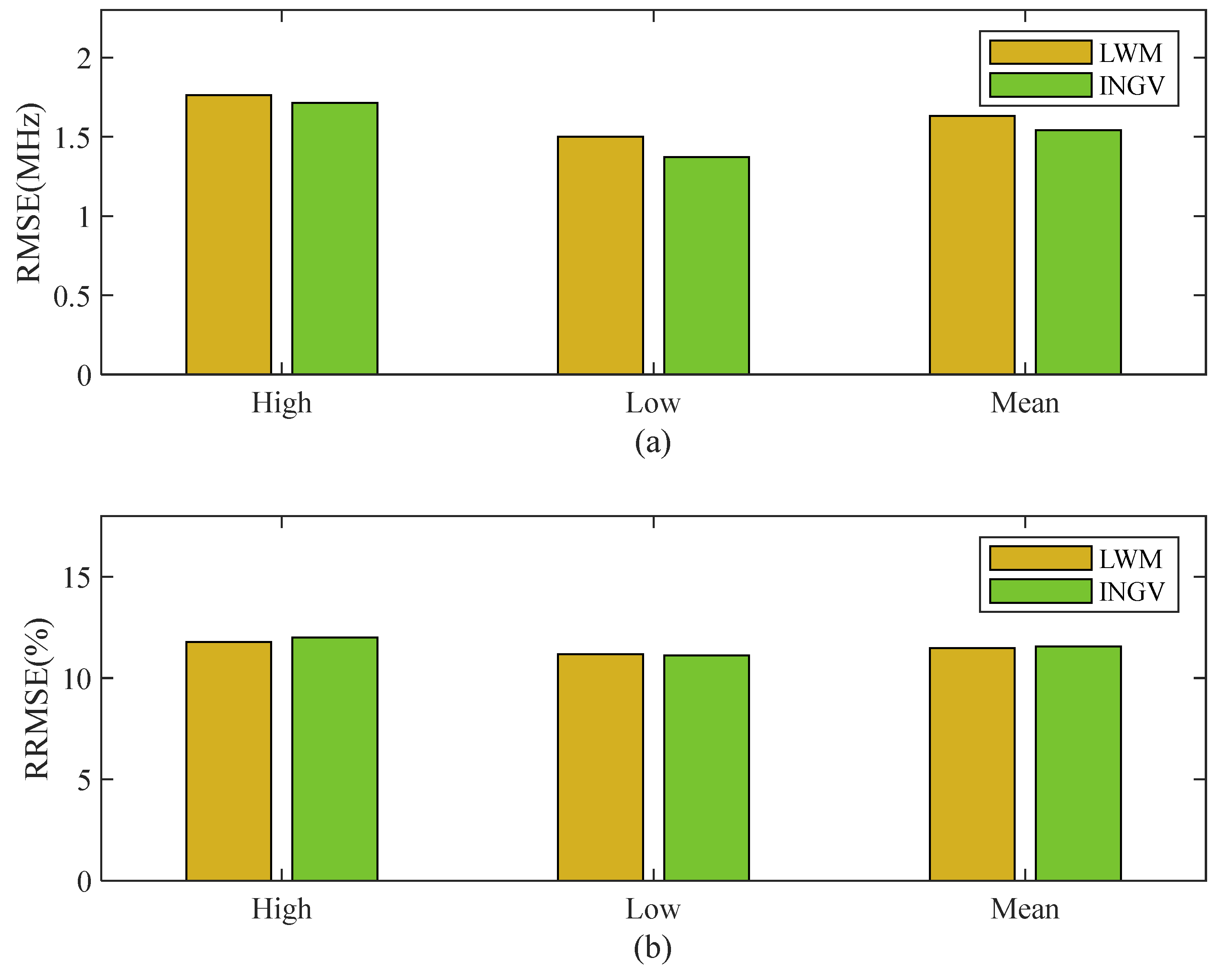
3.3. Models Validation
- Spring includes March, April, and May, and the whole day is divided into four periods: (1) sunrise (5–7 o’clock), (2) daytime (8–16 o’clock), (3) sunset (17–19 o’clock), and (4) nighttime (20–23 and 0–4 o’clock).
- Summer includes June, July, and August, and the whole day is divided into four periods: (1) sunrise (5–7 o’clock), (2) daytime (8–17 o’clock), (3) sunset (18–20 o’clock), and (4) nighttime (21–23 and 0–4 o’clock);
- Autumn includes September, October, and November, and the whole day is divided into four periods: (1) sunrise (5–7 o’clock), (2) daytime (8–16 o’clock), (3) sunset (17–19 o’clock), and (4) nighttime (20–23 and 0–4 o’clock);
- Winter includes December, January, and February; the whole day is divided into four periods: (1) sunrise (6–8 o’clock), (2) daytime (9–16 o’clock), (3) sunset (17–19 o’clock), (4) nighttime (20–23 and 0–5 o’clock).
4. Conclusions
Author Contributions
Funding
Institutional Review Board Statement
Informed Consent Statement
Data Availability Statement
Acknowledgments
Conflicts of Interest
References
- Wang, J.; Ding, G.; Wang, H. HF communications: Past, present, and future. China Commun. 2018, 15, 1–9. [Google Scholar] [CrossRef]
- Yan, Z.; Wang, G.; Tian, G.; Li, W.; Su, D.; Rahman, T. The HF Channel EM Parameters Estimation Under a Complex Environment Using the Modified IRI and IGRF Model. IEEE Trans. Antennas Propagat. 2011, 59, 1778–1783. [Google Scholar] [CrossRef]
- Wang, J.; Yang, C.; An, W. Regional Refined Long-term Predictions Method of Usable Frequency for HF Communication Based on Machine Learning over Asia. IEEE Trans. Antennas Propagat. 2022, 70, 4040–4055. [Google Scholar] [CrossRef]
- International Telecommunication Union. Rec. ITU-R P.373-1 Definitions of Maximum and Minimum Transmission Frequencies; ITU: Geneva, Switzerland, 2008. [Google Scholar]
- Wang, J.; Shi, Y.; Yang, C.; Feng, F. A review and prospects of operational frequency selecting techniques for HF radio communication. Adv. Space Res. 2022, 69, 2989–2999. [Google Scholar] [CrossRef]
- Kallberg, J.; Hamilton, S.S. Resiliency by Retrograded Communication-The Revival of Shortwave as a Military Communication Channel. IT Prof. 2020, 22, 46–51. [Google Scholar] [CrossRef]
- Bilitza, D. IRI the international standard for the ionosphere. Adv. Radio Sci. 2018, 53, 1–11. [Google Scholar] [CrossRef] [Green Version]
- Pietrella, M.; Pezzopane, M.; Zolesi, B.; Cander, L.R.; Pignalberi, A. The Simplified Ionospheric Regional Model (SIRM) for HF Prediction: Basic Theory, Its Evolution and Applications. Surv. Geophy. 2020, 41, 1143–1178. [Google Scholar] [CrossRef]
- Sailors, D.B.; Sprague, R.A.; Rix, W.H. MINIMUF-85: An Improved HF MUF Prediction Algorithm; Naval Ocean Systems Center: San Diego, CA, USA, 1986. [Google Scholar]
- Daehler, M. EINMUF: An HF MUF, FOT, LUF Prediction Program; Naval Research Lab: Washington, DC, USA, 1989. [Google Scholar]
- Roy, T.N.; Sailors, D.B. HF Maximum Usable Frequencies (MUF) Model Uncertainty Assessment; Naval Ocean Systems Center: San Diego, CA, USA, 1987. [Google Scholar]
- Lockwood, M. Simple M-factor algorithm for improved estimation of the basic maximum usable frequency of radio waves reflected from the ionospheric F-region. IEE Proc. F Commun. Radar Signal Process 1983, 130, 296–302. [Google Scholar] [CrossRef]
- International Telecommunication Union. Rec. ITU-R P.1240-1 ITU-R Methods of Basic MUF, Operational MUF and Ray-Path Prediction; ITU: Geneva, Switzerland, 2015. [Google Scholar]
- Zolesi, B.; Fontana, G.; Perrone, L.; Pietrella, M.; Romano, V.; Tutone, G.; Belehaki, A.; Tsagouri, I.; Kouris, S.S.; Vallianatos, F.; et al. A New Campaign for Oblique-Incidence Ionospheric Sounding over Europe and Its Data Application. J. Atmos. Sol.-Terr. Phys. 2008, 70, 854–865. [Google Scholar] [CrossRef]
- Pietrella, M.; Pezzopane, M. Maximum Usable Frequency and Skip Distance Maps over Italy. Adv. Space Res. 2020, 66, 243–258. [Google Scholar] [CrossRef]
- Hadi, K.A.; Goerge, L.E. A Simplified Mathematical Model to Calculate the Maximum Usable Frequencies Over Iraqi Territory. Diyala J. Pure Sci. 2011, 7, 120. [Google Scholar]
- Souza, J.R.; Batista, I.S.; Costa, R.G.D.F. A Simple Method to Calculate the Maximum Usable Frequency. In Proceedings of the 13th International Congress of the Brazilian Geophysical Society & EXPOGEF, Rio de Janeiro, Brazil, 26–29 August 2013. [Google Scholar]
- Nguyen, M.G. Calculation of the Maximum Usable Frequency and Field Strength of Propagation Mode 2F2 Taking into Account the Ionosphere Inhomogeneities. In Proceedings of the 2019 Radiation and Scattering of Electromagnetic Waves, Divnomorskoe, Russia, 24–28 June 2019. [Google Scholar]
- Maltseva, O.A.; Poltavsky, O.S. Evaluation of the IRI model for the European region. Adv. Space Res. 2009, 43, 1638–1643. [Google Scholar] [CrossRef]
- Ahmad, M.; Rashid, I.; Ahmad, N. Validation of MUF and FOT parameters for plain, mountainous and sea region. In Proceedings of the 2015 International Conference on Information and Communication Technologies (ICICT), Karachi, Pakistan, 12–13 December 2015. [Google Scholar]
- Pietrella, M.; Perrone, L.; Fontana, G.; Romano, V.; Malagnini, A.; Tutone, G.; Zolesi, B.; Cander, L.R.; Belehaki, A.; Tsagouri, I.; et al. Oblique-Incidence Ionospheric Soundings over Central Europe and Their Application for Testing Now Casting and Long Term Prediction Models. Adv. Space Res. 2009, 43, 1611–1620. [Google Scholar] [CrossRef]
- Malik, R.A.; Abdullah, M.; Abdullah, S.; Homam, M.J.; Yokoyama, T.; Yatini, C.Y. Prediction and Measurement of High Frequency Radio Frequencies in Peninsular Malaysia and Comparisons with the International Reference Ionosphere Model. Adv. Sci. Lett. 2017, 23, 1294–1298. [Google Scholar] [CrossRef]
- Malik, R.A.; Abdullah, M.; Abdullah, S.; Homan, M.J. Comparison of maximum usable frequency (MUF) variability over Peninsular Malaysia with IRI model during the rise of solar cycle 24. J. Atmos. Sol.-Terr. Phys. 2016, 138–139, 87–92. [Google Scholar] [CrossRef]
- Malik, R.A.; Abdullah, M.; Abdullah, S.; Homan, M.J. Comparison of Measured and Predicted HF Operating Frequencies During Low Solar Activity. In Space Science and Communication for Sustainability; Springer: Singapore, 2018; pp. 73–86. [Google Scholar]
- International Telecommunication Union. Rec. ITU-R P.533-14 Method for the Prediction of the Performance of HF Circuits; ITU: Geneva, Switzerland, 2019. [Google Scholar]
- Reinisch, B.W.; Galkin, I.A. Global Ionospheric Radio Observatory (GIRO). Earth Planet Sp. 2011, 63, 377–381. [Google Scholar] [CrossRef] [Green Version]
- Huang, C.L.; Luo, Y.L.; Huang, R.Y. Oblique Sounding between Digisonde 256 and SSJX-1 Receiver. Chin. J. Radio Sci. 1994, 9, 81–88. [Google Scholar]
- Wang, J.; Ji, S.Y.; Wang, H.F.; Lu, D.M.; Wang, X.Y. Method for determining the critical frequency and propagation factor at the path midpoint from maximum usable frequency and its propagation delay based on oblique sounder. Chin. J. Space Sci. 2014, 34, 160–167. [Google Scholar]
- Chirp Reception and Interpretation. Available online: http://websdr.ewi.utwente.nl:8901/chirps/article (accessed on 15 June 2022).
- Verhulst, T.; Altadill, D.; Mielich, J.; Reinisch, B.; Galkin, I.; Mouzakis, A.; Belehaki, A.; Burešová, D.; Stankov, S.; Blanch, E.; et al. Vertical and Oblique HF Sounding with a Network of Synchronised Ionosondes. Adv. Space Res. 2017, 60, 1644–1656. [Google Scholar] [CrossRef]
- Hervás, M.; Bergadà, P.; Alsina-Pagès, R.M. Ionospheric Narrowband and Wideband HF Soundings for Communications Purposes: A Review. Sensors 2020, 20, 2486. [Google Scholar] [CrossRef]
- Statistic for BEIJING. 25 March 2016. Available online: https://lgdc.uml.edu/common/DIDBDayStationStatistic?ursiCode=BP440&year=2016&month=3&day=25 (accessed on 16 May 2022).
- Wang, J.; Feng, F.; Bai, H.; Cao, Y.; Cheng, Q.; Ma, J. A regional model for the prediction of M(3000)F2 over East Asia. Adv. Space Res. 2020, 65, 2036–2051. [Google Scholar] [CrossRef]
- ISES Solar Cycle Sunspot Number Progression. Available online: https://www.swpc.noaa.gov/products/solar-cycle-progression (accessed on 1 July 2020).


| Model | LWM [12] | INGV [15] | TPM [16] | SPM [17] | NYM [18] |
|---|---|---|---|---|---|
| Applicable scene | 1-hop for ionospheric F2-layer propagation | 1-hop for ionospheric F2-layer propagation | 1-hop for ionospheric F2-layer propagation around the Baghdad station | 1-hop less than 3000 km for ionospheric F2-layer propagation | 1 & 2-hop for ionospheric F2-layer propagation |
| Model input | foE, foF2, and M(3000)F2 at path midpoint | foF2 and M(3000)F2 at path midpoint | Communication distance, local time, month | foF2, hmF2, and TEC below hmF2 at path midpoint | foF2 and the virtual height at [−100, 0, +100] km from the middle point of the circuit |
| Characteristics | Most widely used in the world | Most concise and easier to implement | Only applicable for the monthly median value over the Iraqi region | The total electron content (TEC) below hmF2 can sometimes not be directly measured | Relatively complex calculation |
| Parameters | The Performance Parameters |
|---|---|
| Sounding frequency | 2–30 MHz |
| Working mode | Linear or logarithmic sweep |
| Signal types | Pulse code |
| Sounding period | ≤60 min |
| Sounding altitude | 80–1200 km |
| Height resolution | ≤5 km |
| Synchronization mode | GPS |
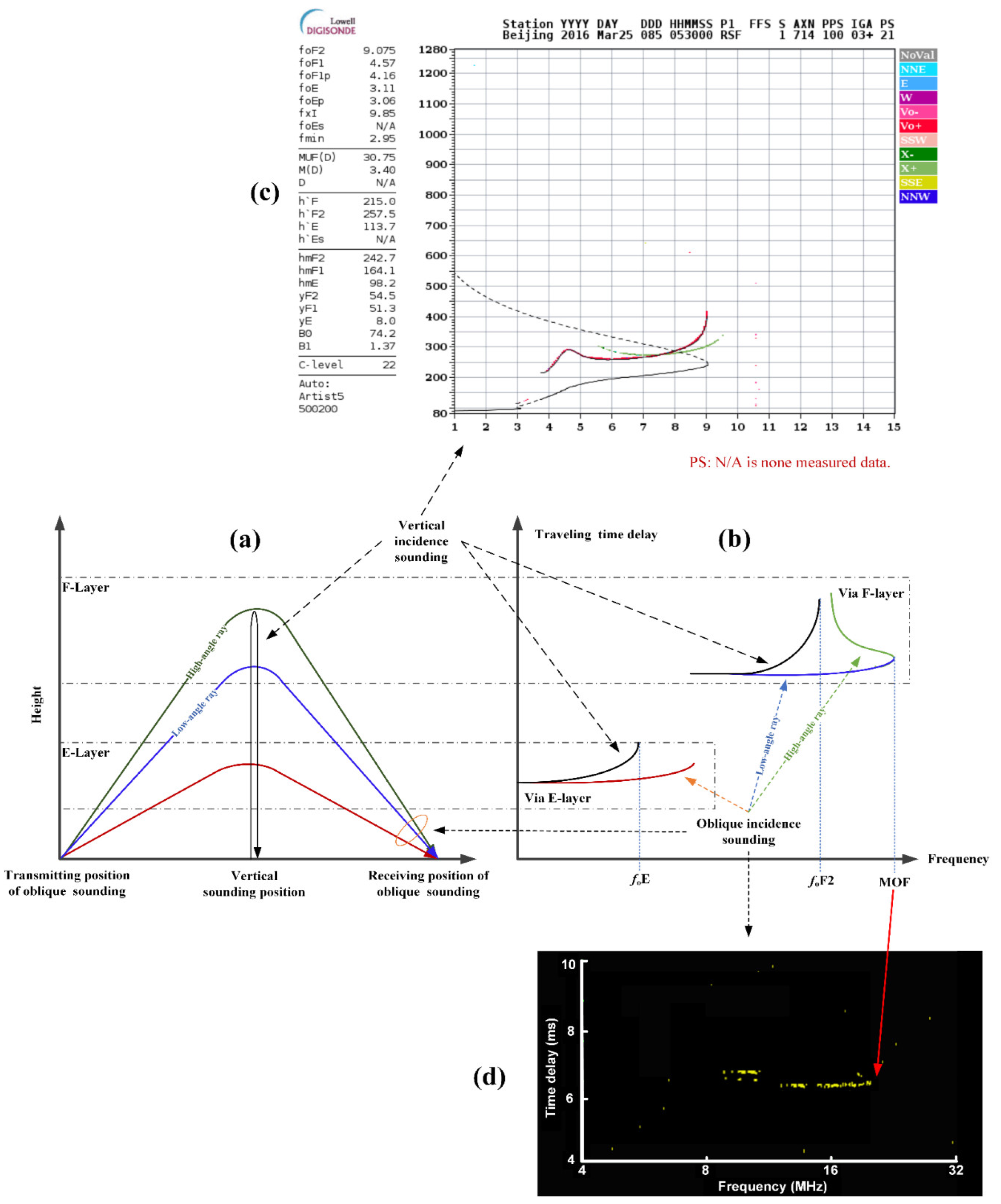
| Parameters output | Diagram of Signal delay against frequency (see the Figure 1c) |
| Data output | foE, foF2, hmE, hmF2, M(3000)F2 etc. |
| Parameters | The Performance Parameters |
|---|---|
| Operating frequency | 2–30 MHz |
| Working mode | Linear or logarithmic sweep |
| Sounding period | ≤60 min |
| Synchronization mode | GPS |
| Parameters output | Diagram of signal delay and energy against frequency (see Figure 1d) |
| Data output | Lowest observed frequency (LOF) and MOF |
Publisher’s Note: MDPI stays neutral with regard to jurisdictional claims in published maps and institutional affiliations. |
© 2022 by the authors. Licensee MDPI, Basel, Switzerland. This article is an open access article distributed under the terms and conditions of the Creative Commons Attribution (CC BY) license (https://creativecommons.org/licenses/by/4.0/).
Share and Cite
Wang, J.; Shi, Y.; Yang, C. Investigation of Two Prediction Models of Maximum Usable Frequency for HF Communication Based on Oblique- and Vertical-Incidence Sounding Data. Atmosphere 2022, 13, 1122. https://doi.org/10.3390/atmos13071122
Wang J, Shi Y, Yang C. Investigation of Two Prediction Models of Maximum Usable Frequency for HF Communication Based on Oblique- and Vertical-Incidence Sounding Data. Atmosphere. 2022; 13(7):1122. https://doi.org/10.3390/atmos13071122
Chicago/Turabian StyleWang, Jian, Yafei Shi, and Cheng Yang. 2022. "Investigation of Two Prediction Models of Maximum Usable Frequency for HF Communication Based on Oblique- and Vertical-Incidence Sounding Data" Atmosphere 13, no. 7: 1122. https://doi.org/10.3390/atmos13071122