
Seismo-Ionospheric Effects Prior to Two Earthquakes in Taiwan Detected by the China Seismo-Electromagnetic Satellite
 , , ,
, , ,
Abstract
:1. Introduction
2. Datasets
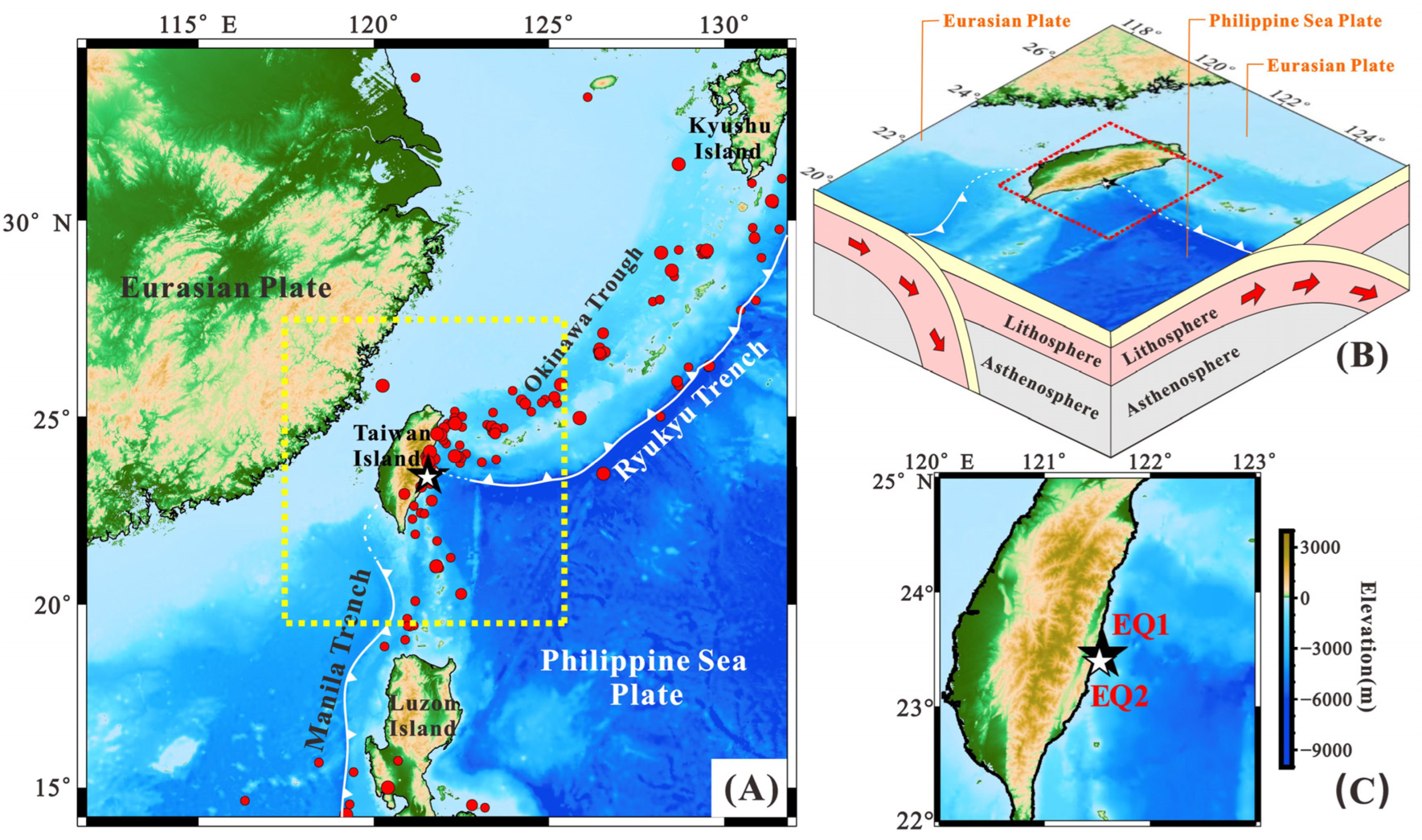
2.1. Seismic Events
2.2. Ne Data Acquired by the LAP Onboard the CSES
2.3. CODE TEC Data
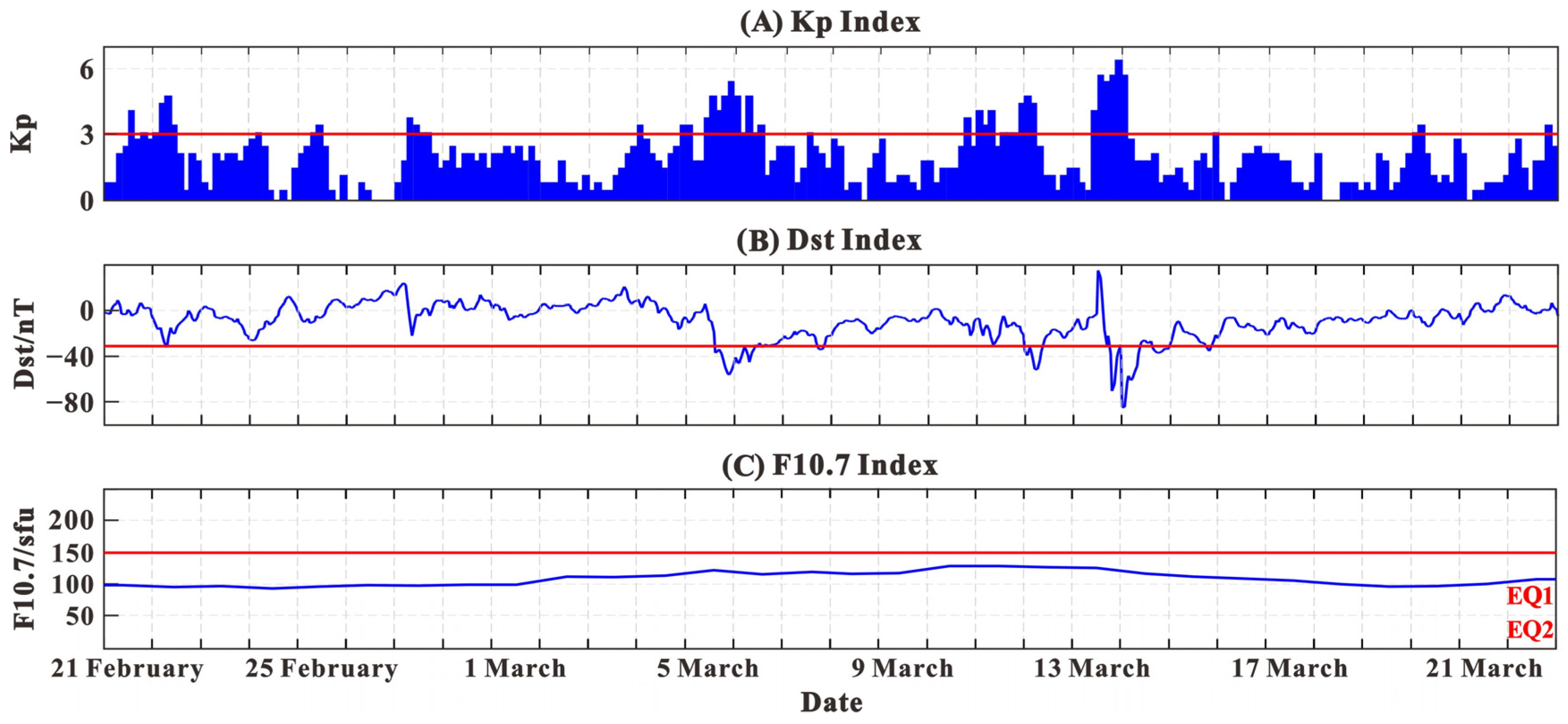
2.4. Solar-Geomagnetic Data
3. Analysis and Results
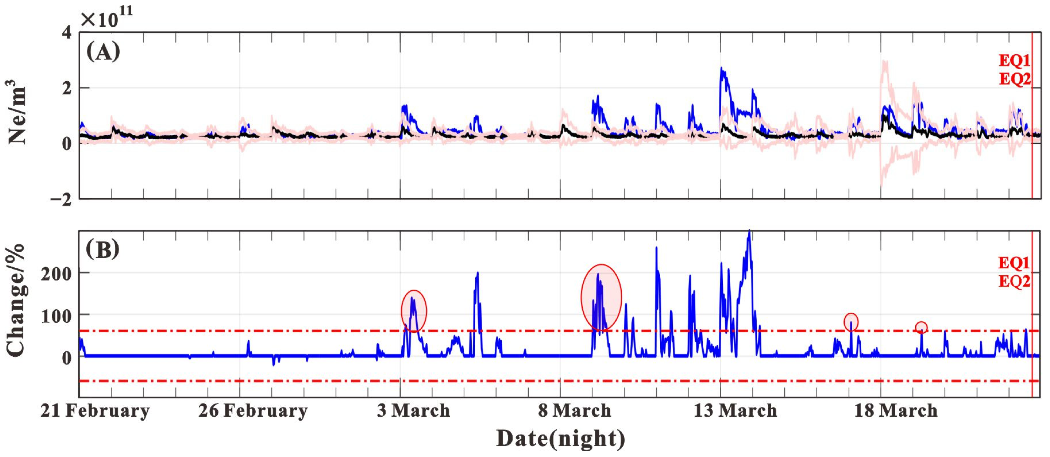
3.1. Time-Series Analysis of CSES Ne Data
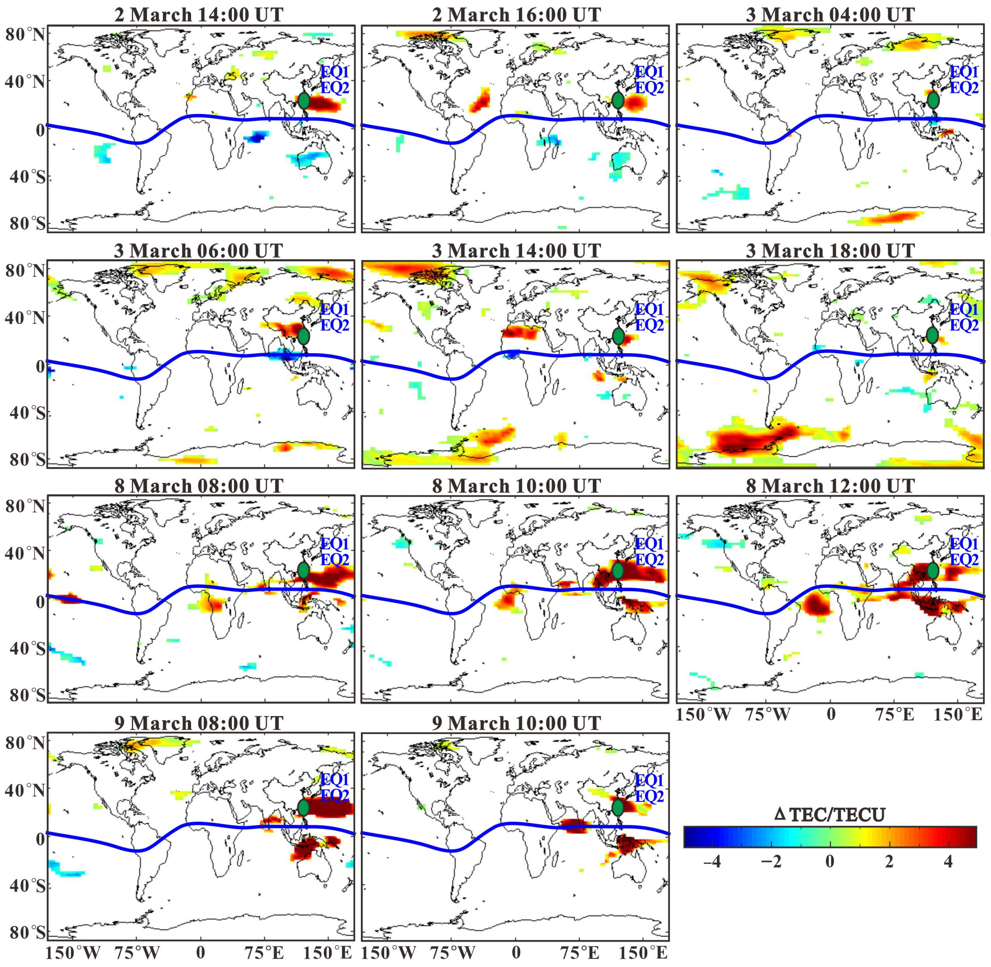
3.2. Analysis of CODE TEC Mapping Data
4. Statistical Analysis
5. Discussion
6. Conclusions
Author Contributions
Funding
Institutional Review Board Statement
Informed Consent Statement
Data Availability Statement
Acknowledgments
Conflicts of Interest
References
- Zhang, X.M.; Shen, X.H.; Zhao, S.F.; Liu, J.; Ouyang, X.Y.; Lou, W.Y.; Zeren, Z.M.; He, J.H.; Qian, G. The seismo-ionospheric monitoring technologies and their application research development. Acta Seismol. Sin. 2016, 38, 356–375, (In Chinese with an English abstract). [Google Scholar]
- Leonard, R.S.; Barnes, R.A. Observation of ionospheric disturbances following the Alaska earthquake. J. Geophys. Res. 1965, 70, 1250–1253. [Google Scholar] [CrossRef]
- Pulinets, S.A. Strong earthquake prediction possibility with the help of topside sounding from satellites. Adv. Space Res. 1998, 21, 455–458. [Google Scholar] [CrossRef]
- Liu, J.Y.; Chen, Y.I.; Pulinets, S.A.; Tsai, Y.B.; Chuo, Y.J. Seismo-ionospheric signatures prior to M ≥ 6.0 Taiwan earthquakes. Geophys. Res. Lett. 2000, 27, 3113–3116. [Google Scholar] [CrossRef]
- Singh, O.P.; Chauhan, V.; Singh, V.; Singh, B. Anomalous variation in total electron content (TEC) associated with earthquakes in India during September 2006-November 2007. Phys. Chem. Earth 2009, 34, 479–484. [Google Scholar] [CrossRef]
- Shah, M.; Jin, S. Statistical characteristics of seismo-ionospheric GPS TEC disturbances prior to global MW > 5.0 earthquakes (1998–2014). J. Geodyn. 2015, 92, 42–49. [Google Scholar] [CrossRef]
- Benghanem, K.; Kahlouche, S.; Abtout, A.; Beldjoudi, H. The cross correlation method response prior to earthquakes using foF2 data from various ionospheric stations. Adv. Space Res. 2019, 63, 2638–2658. [Google Scholar] [CrossRef]
- Li, M.; Shen, X.H.; Parrot, M.; Zhang, X.M.; Zhang, Y.; Yu, C.; Yan, R.; Liu, D.P.; Lu, H.X.; Guo, F.; et al. Primary joint statistical seismic influence on ionospheric parameters recorded by the CSES and DEMETER satellites. J. Geophys. Res. Space Phys. 2020, 125, A028116. [Google Scholar] [CrossRef]
- Pulinets, S.A.; Boyarchuk, K. Ionospheric Precursors of Earthquakes; Springer: Berlin/Heidelberg, Germany, 2004; pp. 75–169. [Google Scholar]
- Liu, J.; Lou, W.Y.; Zhang, X.M.; Shen, X.H. A comparison study of foF2 derived from oblique sounding network and vertical ionosonde in Northern China. Terr. Atmos. Ocean. Sci. 2016, 27, 933–941. [Google Scholar] [CrossRef]
- Ahmed, J.; Shah, M.; Awais, M.; Jin, S.G.; Zafar, W.A.; Ahmad, N.; Amin, A.; Shah, M.A.; Ali, I. Seismo-ionospheric anomalies before the 2019 Mirpur earthquake from ionosonde measurements. Adv. Space Res. 2022, 69, 26–34. [Google Scholar] [CrossRef]
- Calais, E.; Minster, J.B. GPS detection of ionospheric perturbations following the January 17, 1994, Northridge earthquake. Geophys. Res. Lett. 1995, 22, 1045–1048. [Google Scholar] [CrossRef]
- Zhao, B.Q.; Wang, M.; Yu, T.; Wan, W.X.; Lei, J.H.; Liu, L.B.; Ning, B.Q. Is an unusual large enhancement of ionospheric electron density linked with the 2008 great Wenchuan earthquake? J. Geophys. Res. 2008, 113, A11304. [Google Scholar] [CrossRef]
- Chen, Y.I.; Huang, C.S.; Liu, J.Y. Statistical evidences of seismo-ionospheric precursors applying receiver operating characteristic (ROC) curve on the GPS total electron content in China. J. Asian Earth Sci. 2015, 114, 393–402. [Google Scholar] [CrossRef]
- Song, R.; Zhang, X.M.; Zhou, C.; Liu, J.; He, J.H. Predicting TEC in China based on the neural networks optimized by genetic algorithm. Adv. Space Res. 2018, 62, 745–759. [Google Scholar] [CrossRef]
- Simha, C.P.; Natarajan, V.; Rao, K.M. Pre-earthquake atmospheric and ionospheric anomalies before Taiwan earthquakes (M 6.1 and M 6.4) on February (4th and 6th), 2018. Geomagn. Aeron. 2020, 60, 644–660. [Google Scholar] [CrossRef]
- Hayakawa, M.; Kasahara, Y.; Nakamura, T.; Muto, F.; Horie, T.; Maekawa, S.; Hobara, Y.; Rozhnoi, A.A.; Solovieva, M.; Molchanov, O.A. A statistical study on the correlation between lower ionospheric perturbations as seen by subionospheric VLF/LF propagation and earthquakes. J. Geophys. Res. 2010, 115, A09305. [Google Scholar] [CrossRef]
- Zeren, Z.M.; Zhang, X.M.; Shen, X.H.; Sun, W.H.; Ning, D.M.; Yuri, R. VLF radio signal anomalies associated with strong earthquakes. In Proceedings of the 2014 XXXIth URSI General Assembly and Scientific Symposium, Beijing, China, 16–23 August 2014; IEEE: Manhattan, NY, USA, 2014; pp. 1–4. [Google Scholar] [CrossRef]
- Hayakawa, M.; Ohta, K.; Nickolaenko, A.P.; Ando, Y. Anomalous effect in Schumann resonance phenomena observed in Japan, possibly associated with the Chi-chi earthquake in Taiwan. Ann. Geophys. 2005, 23, 1335–1346. [Google Scholar] [CrossRef]
- Ouyang, X.Y.; Xiao, Z.; Hao, Y.Q.; Zhang, D.H. Variability of Schumann resonance parameters observed at low latitude stations in China. Adv. Space Res. 2015, 56, 1389–1399. [Google Scholar] [CrossRef]
- Pulinets, S.A.; Legen’ka, A.D. Spatial-temporal characteristics of large scale disturbances of electron density observed in the ionospheric F-region before strong earthquakes. Cosm. Res. 2003, 41, 221–229. [Google Scholar] [CrossRef]
- Zeren, Z.M.; Shen, X.H.; Zhang, X.M.; Cao, J.B.; Huang, J.P.; Ouyang, X.Y.; Liu, J.; Bingqing, L. Possible ionospheric electromagnetic perturbations induced by the MS 7.1 Yushu earthquake. Earth Moon Planets 2012, 108, 234–241. [Google Scholar] [CrossRef]
- Liu, J.; Zhang, X.M.; Novikov, V.; Shen, X.H. Variations of ionospheric plasma at different altitudes before the 2005 Sumatra Indonesia MS 7.2 earthquake. J. Geophys. Res. Space Phys. 2016, 121, 9179–9187. [Google Scholar] [CrossRef]
- He, Y.F.; Zhao, X.D.; Yang, D.M.; Wu, Y.Y.; Li, Q. A study to investigate the relationship between ionospheric disturbance and seismic activity based on Swarm satellite data. Phys. Earth Planet. Inter. 2022, 323, 106826. [Google Scholar] [CrossRef]
- Yan, R.; Shen, X.H.; Huang, J.P.; Wang, Q.; Chu, W.; Liu, D.P.; Yang, Y.Y.; Lu, H.X.; Xu, S. Examples of unusual ionospheric observations by the CSES prior to earthquakes. Earth Planet. Phys. 2018, 2, 515–526. [Google Scholar] [CrossRef]
- Zhang, X.M.; Wang, Y.L.; Boudjada, M.Y.; Liu, J.; Magnes, W.; Zhou, Y.L.; Du, X.H. Multi-experiment observations of ionospheric disturbances as precursory effects of the Indonesian MS 6.9 earthquake on August 05, 2018. Remote Sens. 2020, 12, 4050. [Google Scholar] [CrossRef]
- Song, R.; Hattori, K.; Zang, X.M.; Sanaka, S. Seismic-ionospheric effects prior to four earthquakes in Indonesia detected by the China seismo-electromagnetic satellite. J. Atmos. Sol. Terr. Phys. 2020, 205, 105291. [Google Scholar] [CrossRef]
- Xie, T.; Chen, B.Y.; Wu, L.X.; Dai, W.J.; Kuang, C.L.; Miao, Z.L. Detecting seismo-ionospheric anomalies possibly associated with the 2019 Ridgecrest (California) earthquakes by GNSS, CSES, and Swarm observations. J. Geophys. Res. Space Phys. 2021, 126, A028761. [Google Scholar] [CrossRef]
- Zhang, X.M.; Liu, J.; Xiong, P.; Zhou, Y.L. The seismo-ionospheric disturbances before the 2020 Yutian MS 6.4 earthquake. Earthquake 2021, 41, 145–157, (In Chinese with an English abstract). [Google Scholar]
- Du, X.H.; Zhang, X.M. Ionospheric disturbances possibly associated with Yangbi MS 6.4 and Maduo MS 7.4 earthquakes in China from China seismo electromagnetic satellite. Atmosphere 2022, 13, 438. [Google Scholar] [CrossRef]
- Chen, P.F.; Huang, B.S.; Chiao, L.Y. Upper mantle seismic velocity anomaly beneath southern Taiwan as revealed by teleseismic relative arrival times. Tectonophysics 2011, 498, 27–34. [Google Scholar] [CrossRef]
- Zhu, K.Y.; Zheng, L.; Yan, R.; Shen, X.H.; Zeren, Z.M.; Xu, S.; Chu, W.; Liu, D.P.; Zhou, N.; Guo, F. Statistical study on the variations of electron density and temperature related to seismic activities observed by CSES. Nat. Hazards Res. 2021, 1, 88–94. [Google Scholar] [CrossRef]
- Huang, H.; Yan, R.; Liu, D.P.; Xu, S.; Lin, J.; Guo, F.; Huang, J.P.; Zeren, Z.M.; Shen, X.H. The variations of plasma density recorded by CSES-1 satellite possibly related to Mexico MS 7.1 earthquake on 8th September 2021. Nat. Hazards Res. 2022, 2, 11–16. [Google Scholar] [CrossRef]
- Dobrovolsky, I.P.; Zubkov, S.I.; Miachkin, V.I. Estimation of the size of earthquake preparation zones. Pure Appl. Geophys. 1979, 117, 1025–1044. [Google Scholar] [CrossRef]
- Saito, A.; Fukao, S.; Miyazaki, S. High resolution mapping of TEC perturbations with the GSI GPS network over Japan. Geophys. Res. Lett. 1998, 25, 3079–3082. [Google Scholar] [CrossRef]
- Tsugawa, T.; Otsuka, Y.; Coster, A.J.; Saito, A. Medium-scale traveling ionospheric disturbances detected with dense and wide TEC maps over North America. Geophys. Res. Lett. 2007, 34, L22101. [Google Scholar] [CrossRef]
- Ding, F.; Wan, W.X.; Xu, G.; Yu, T.; Yang, G.L.; Wang, J.S. Climatology of medium-scale traveling ionospheric disturbances observed by a GPS network in central China. J. Geophys. Res. 2011, 116, A09327. [Google Scholar] [CrossRef]
- Lee, C.C.; Liou, Y.A.; Otsuka, Y.; Chu, F.D.; Yeh, T.K.; Hoshinoo, K.; Matunaga, K. Nighttime medium-scale traveling ionospheric disturbances detected by network GPS receivers in Taiwan. J. Geophys. Res. 2008, 113, A12316. [Google Scholar] [CrossRef]
- Liu, J.Y.; Chen, C.H.; Chen, Y.I.; Yang, W.H.; Oyama, K.I.; Kuo, K.W. A statistical study of ionospheric earthquake precursors monitored by using equatorial ionization anomaly of GPS TEC in Taiwan during 2001-2007. J. Asian Earth Sci. 2010, 39, 76–80. [Google Scholar] [CrossRef]
- Chen, C.H.; Liu, J.Y.; Yumoto, K.; Lin, C.H.; Fang, T.W. Equatorial ionization anomaly of the total electron content and equatorial electrojet of ground-based geomagnetic field strength. J. Atmos. Sol. Terr. Phys. 2008, 70, 2172–2183. [Google Scholar] [CrossRef]
- Fang, T.W.; Richmond, A.D.; Liu, J.Y.; Maute, A.; Lin, C.H.; Chen, C.H.; Harper, B. Model simulation of the equatorial electrojet in the Peruvian and Philippine sectors. J. Atmos. Sol. Terr. Phys. 2008, 70, 2203–2211. [Google Scholar] [CrossRef]
- Fang, T.W.; Richmond, A.D.; Liu, J.Y.; Maute, A. Wind dynamo effects on ground magnetic perturbations and vertical drifts. J. Geophys. Res. 2008, 113, A11313. [Google Scholar] [CrossRef]
- Liu, J.Y.; Chen, Y.I.; Chuo, Y.J.; Tsai, H.F. Variations of ionospheric total electron content during the Chi-chi earthquake. Geophys. Res. Lett. 2001, 28, 1383–1386. [Google Scholar] [CrossRef] [Green Version]
- Liu, J.Y.; Chuo, Y.J.; Shan, S.J.; Tsai, Y.B.; Chen, Y.I.; Pulinets, S.A.; Yu, S.B. Pre-earthquake ionospheric anomalies registered by continuous GPS TEC measurements. Ann. Geophys. 2004, 22, 1585–1593. [Google Scholar] [CrossRef]
- Liu, J.Y.; Chen, Y.I.; Jhuang, H.K.; Lin, Y.H. Ionospheric foF2 and TEC anomalous days associated with M ≥ 5.0 earthquakes in Taiwan during 1997-1999. Terr. Atmos. Ocean Sci. 2004, 15, 371–384. Available online: https://irsl.ss.ncu.edu.tw/media/paper/2004054.pdf (accessed on 1 August 2022). [CrossRef]
- Liu, J.Y.; Chen, Y.I.; Chuo, Y.J.; Chen, C.S. A statistical investigation of preearthquake ionospheric anomaly. J. Geophys. Res. 2006, 111, A05304. [Google Scholar] [CrossRef]
- Du, X.H. Application of Strong Earthquake Research Based on Multiple Parameters of Space Electromagnetism. Master’s Thesis, Institute of Earthquake Forecasting, China Earthquake Administration, Beijing, China, 20 June 2022. (In Chinese with an English abstract). [Google Scholar]
- Gutenberg, B. The energy of earthquakes. Q. J. Geol. Soc. 1956, 112, 1–14. [Google Scholar] [CrossRef]
- Zhang, X.M.; Shen, X.H. The development in seismo-ionospheric coupling mechanism. Prog. Earthq. Sci. 2022, 52, 193–202, (In Chinese with an English abstract). [Google Scholar]
- Hayakawa, M. Electromagnetic phenomena associated with earthquakes: A frontier in terrestrial electromagnetic noise environment. Recent Res. Dev. Geophys. 2004, 6, 81–112. [Google Scholar]
- Ding, J.H.; Shen, X.H.; Pan, W.Y.; Zhang, J.; Yu, S.R.; Li, G.; Guan, H.P. Seismo-electromagnetism precursor research progress. Chin. J. Radio Sci. 2006, 21, 791–801, (In Chinese with an English abstract). [Google Scholar]
- Pulinets, S.; Ouzounov, D. Lithosphere-Atmosphere-Ionosphere Coupling (LAIC) model: An unified concept for earthquake precursors validation. J. Asian Earth Sci. 2011, 41, 371–382. [Google Scholar] [CrossRef]
- Wu, L.X.; Qin, K.; Liu, S.J. GEOSS-based thermal parameters analysis for earthquake anomaly recognition. Proc. IEEE 2012, 100, 2891–2907. [Google Scholar] [CrossRef]
- Liao, L.X.; Chen, L.; Zhang, J.F. The analysis of effective earthquake reflecting factor of Fujian fluid net to Taiwan earthquakes with MS 7.0. Earthquake 2006, 26, 95–103, (In Chinese with an English abstract). [Google Scholar]
- King, C.Y.; Chia, Y. Anomalous streamflow and groundwater-level changes before the 1999 M 7.6 Chi-chi earthquake in Taiwan: Possible mechanisms. Pure Appl. Geophys. 2017, 175, 2435–2444. [Google Scholar] [CrossRef]
- Genzano, N.; Filizzola, C.; Paciello, R.; Pergola, N.; Tramutoli, V. Robust Satellite Techniques (RST) for monitoring earthquake prone areas by satellite TIR observations: The case of 1999 Chi-chi earthquake (Taiwan). J. Asian Earth Sci. 2015, 114, 289–298. [Google Scholar] [CrossRef]
- Yuan, Y.; Yin, J.Y.; Li, C.F.; Song, Y.; Zhou, S.Q.; Zhao, J.J.; Sun, X.K.; Fang, G.Q. Thermal infrared anomalies of satellite in Taiwan, Xinbei’s MS 6.2 earthquake based on SST background field. Prog. Geophys. 2019, 34, 500–508, (In Chinese with an English abstract). [Google Scholar]
- Lin, G.Y. The anomalous changes of subsurface fluid in Fujian before Taidong MS 7.0 earthquake in Taiwan Province. Seismol. Geomagn. Obs. Res. 2004, 25, 30–35, (In Chinese with an English abstract). [Google Scholar]
- Qian, S.Q.; Hao, J.Q.; Zhou, J.G.; Gao, J.T.; Wang, M.L.; Liang, J. ULF electromagnetic precursors before 1999 Jiji, Taiwan earthquake and the comparison with results of simulating experiments. Acta Seismol. Sin. 2001, 23, 322–327, (In Chinese with an English abstract). [Google Scholar] [CrossRef]
- Zhou, Z.R.; Lü, J.; Zhou, B. Earthquake Prediction Index System in South China; Seismological Press: Beijing, China, 2021; pp. 184–235. (In Chinese) [Google Scholar]


| No. | BJT | UT | Lat./°N | Lon./°E | Depth/km | Magnitude |
|---|---|---|---|---|---|---|
| EQ1 | 23 March 2022 01:41:38 | 22 March 2022 17:41:38 | 23.45 | 121.55 | 20 | 6.7 |
| EQ2 | 23 March 2022 04:29:58 | 22 March 2022 20:29:58 | 23.39 | 121.52 | 20 | 6.3 |
| Magnitude | Number of Seismic Groups | Total Anomalies | Anomalies before Earthquakes | Anomalies after Earthquakes | |||
|---|---|---|---|---|---|---|---|
| Number | Frequency | Number | Frequency | Number | Frequency | ||
| 5.0–5.4 | 36 | 65 | 1.81 | 42 | 1.17 | 23 | 0.64 |
| 5.5–5.9 | 14 | 41 | 2.93 | 30 | 2.14 | 11 | 0.79 |
| 6.0–6.4 | 7 | 15 | 2.14 | 11 | 1.57 | 4 | 0.57 |
| 6.5–6.9 | 8 | 28 | 3.50 | 19 | 2.38 | 9 | 1.13 |
| Total | 65 | 149 | 2.30 | 102 | 1.57 | 47 | 0.72 |
| Basic Information | Description of Anomaly | Relationship between the Anomaly and EQ1 and EQ2 | |||||
|---|---|---|---|---|---|---|---|
| Well | Index | Lat./°N | Lon./°E | Start and End Time (BJT) | Character Description | Number of Days between the Occurrence of the Anomaly and EQ1 and EQ2/d | Distance/km |
| Xiamen Dongfu | F− | 24.5 | 117.9 | 5 March 2022 | >1.6 σ (standard deviation) | 18 | 387 |
| Ningde | Gas radon | 26.7 | 119.5 | 31 January–24 February 2022 | The gas radon concentration occurred, but the temperature did not change. | 51 | 411 |
| Huaan Tainei | Water radon | 24.7 | 117.6 | 11 February 2022 | The water radon value was higher than 90 Bq/L and oscillated strongly. The temperature was normal. | 40 | 430 |
Publisher’s Note: MDPI stays neutral with regard to jurisdictional claims in published maps and institutional affiliations. |
© 2022 by the authors. Licensee MDPI, Basel, Switzerland. This article is an open access article distributed under the terms and conditions of the Creative Commons Attribution (CC BY) license (https://creativecommons.org/licenses/by/4.0/).
Share and Cite
Guo, Y.; Zhang, X.; Liu, J.; Yang, M.; Yang, X.; Du, X.; Lü, J.; Xiao, J. Seismo-Ionospheric Effects Prior to Two Earthquakes in Taiwan Detected by the China Seismo-Electromagnetic Satellite. Atmosphere 2022, 13, 1523. https://doi.org/10.3390/atmos13091523
Guo Y, Zhang X, Liu J, Yang M, Yang X, Du X, Lü J, Xiao J. Seismo-Ionospheric Effects Prior to Two Earthquakes in Taiwan Detected by the China Seismo-Electromagnetic Satellite. Atmosphere. 2022; 13(9):1523. https://doi.org/10.3390/atmos13091523
Chicago/Turabian StyleGuo, Yufan, Xuemin Zhang, Jiang Liu, Muping Yang, Xing Yang, Xiaohui Du, Jian Lü, and Jian Xiao. 2022. "Seismo-Ionospheric Effects Prior to Two Earthquakes in Taiwan Detected by the China Seismo-Electromagnetic Satellite" Atmosphere 13, no. 9: 1523. https://doi.org/10.3390/atmos13091523