Attention-Based BiLSTM Model for Pavement Temperature Prediction of Asphalt Pavement in Winter

Abstract

Pavement temperature is the main factor determining road icing, and accurate and timely pavement temperature prediction is of significant importance to regional traffic safety management and preventive maintenance. The prediction of pavement temperature at the micro-scale has been a challenge to be tackled. To solve this problem, a bidirectional extended short-term memory network model based on the attention mechanism (Att-BiLSTM) was proposed to improve the prediction performance by using the time series features of pavement temperature and meteorological factors. Pavement temperature data and climatic data were collected from a road weather station in Yunnan, China. The results show that the MAE, MSE, and MAPE of the proposed Att-BiLSTM model were 0.330, 0.339, and 10.1%, respectively, which were better than the other baseline models. It was shown that 93.4% of the predicted values had an error less than 1 °C, and 82.1% had an error less than 0.5 °C, indicating that the proposed Att-BiLSTM model enables significant performance improvement. In addition, this paper quantified and analyzed the effects of parameters such as the size of the sliding window, the number of hidden layer neurons, and the optimizer on the performance of the prediction model.

1. Introduction

Road surface conditions have a significant impact on the safe operation of vehicles [1,2]. Especially in winter, rain and snow tend to cause the road surface to freeze, which can significantly reduce the friction coefficient of asphalt pavement and create poor road pavement driving conditions, which can cause serious traffic accidents. In winter, pavement temperature is a significant factor determining road icing, and the accurate prediction of pavement temperature can provide guidance for preventive and proactive pavement maintenance and improve service levels [3,4]. For example, real-time data from pavement condition monitoring systems can be used to predict future pavement temperatures and salt dangerous road sections before they are at risk of icing up, preventing the risk before it happens.

Pavement temperature prediction is a nonstationary time series prediction problem, and traditional methods usually only rely on a previous moment of observation for prediction, such as the Markov model and the autoregressive moving average model. These methods cannot consider the thermal inertia of a pavement, so the accuracy of the models is poor. With the rise in machine learning models, especially recurrent neural networks (RNNs), RNNs have made a major breakthrough in time series forecasting because RNNs can find and model higher-order nonlinear relationships in time series. Although researchers have applied RNNs and other deep learning models to pavement temperature prediction, the meteorological factors affecting pavement temperature are less considered in the models, so the influence of meteorological elements on pavement temperature is not well modeled.

In this paper, a bi-directional long short-term memory (BiLSTM) model based on an attention mechanism was proposed that is practical and implementable. The BiLSTM can effectively solve the gradient disappearance and gradient explosion problems and is used to capture the forward and reverse information of the sequence more completely [5]. Attentional mechanisms were used to precisely identify the most important features. The proposed model has the ability to accurately predict pavement temperatures using historical pavement temperature data and can provide support for preventive maintenance.

2. Literature Review

Most of the existing studies solved the pavement temperature prediction problem in different ways, using both physical and statistical models.

Physical models are used to predict pavement temperatures by solving partial differential equations for heat transfer. For example, Sass developed a surface energy equation in 1992 to predict pavement temperatures over a 3 h period [6]. Voldborg developed a forecasting model that can generate short-term indicators such as air temperature, humidity, and road surface temperature for each of the more than 200 road weather stations in Denmark [7]. Meng developed a refined numerical model for the prediction of pavement parameters, taking into account the influence of pavement factors and basic urban properties, and the results showed that solar radiation correction factors, asphalt depth, and asphalt thermal conductivity are important parameters for the simulation of road interface temperatures [8]. Chen J et al. proposed an innovative time-varying function to predict pavement temperature in relation to solar radiation and air temperature [9]. However, the physical model is complex to model and requires a large number of difficult-to-collect parameters as input. At the same time, as Karsistoa’s results show, errors can be significant when physical variations are complex [10].

In contrast to physical models, statistical models do not require analytical deviations and numerical calculations to estimate pavement temperatures, but rather statistical analysis based on historical data to obtain a reasonable predictive model. Statistical models are divided into linear and nonlinear models depending on the relationship between the influencing factors and the pavement temperature. For example, Park et al. developed a linear regression model for estimating the minimum surface temperature of a pavement based on the ambient air temperature [11]. Asefzadeh et al. developed separate models for predicting daily average pavement temperatures for different seasons and daily maximum and minimum pavement temperatures for different asphalt layer depths [12]. Kršmanc et al. adjusted the input parameters and different time intervals to predict pavement temperatures based on stepwise linear regression analysis [13]. Zapata et al. developed a medium-depth pavement temperature prediction model and conducted a sensitivity analysis on the influencing factors, and found that there is a nonlinear relationship between the influencing factors and the pavement temperature [14]. In contrast to the linear regression model, nonlinear regression models both typically involve more complex equations and better capture the nonlinear relationship between pavement temperature and the influencing factors, which makes it the classical model in this field.

With the rise in machine learning models, many promising methods have been widely used to model pavement temperatures. Yang et al. used K-Nearest Neighbors to explore the variation in pavement temperature on different road sections [15]. Molavi et al. evaluated the performance of different machine learning models for the prediction of asphalt pavement temperatures under average, minimum, and maximum daily temperatures [16]. Milad et al. proposed an asphalt pavement temperature prediction model through deep learning techniques and suggested that future researchers should integrate loss-balancing algorithms into multi-task learning to improve the efficiency of difficult tasks. Meanwhile, future studies of predicted pavement temperatures should consider the effects of factors such as air temperature, wind speed, and relative humidity [17]. Li et al. proposed that the prediction of pavement surface temperature should not be a single value, but a probability distribution. They developed a prediction model for evaluating the probability distribution of pavement surface temperature in winter [18].

3. Objective and General Outline

3.1. Objective

The present study aimed to proposes an attention-based BiLSTM model for the pavement temperature prediction of asphalt pavement in winter. The BiLSTM was used to completely capture the forward and reverse information of pavement temperature sequences and meteorological feature sequences, and the attention mechanism was used to accurately identify the most important features and improve feature utilization to further improve the performance of pavement temperature prediction. In addition, this study analyzed the effects of the size of the sliding window, the number of hidden layer neurons, the optimizer, and the training epoch on the prediction accuracy.

3.2. General Outline

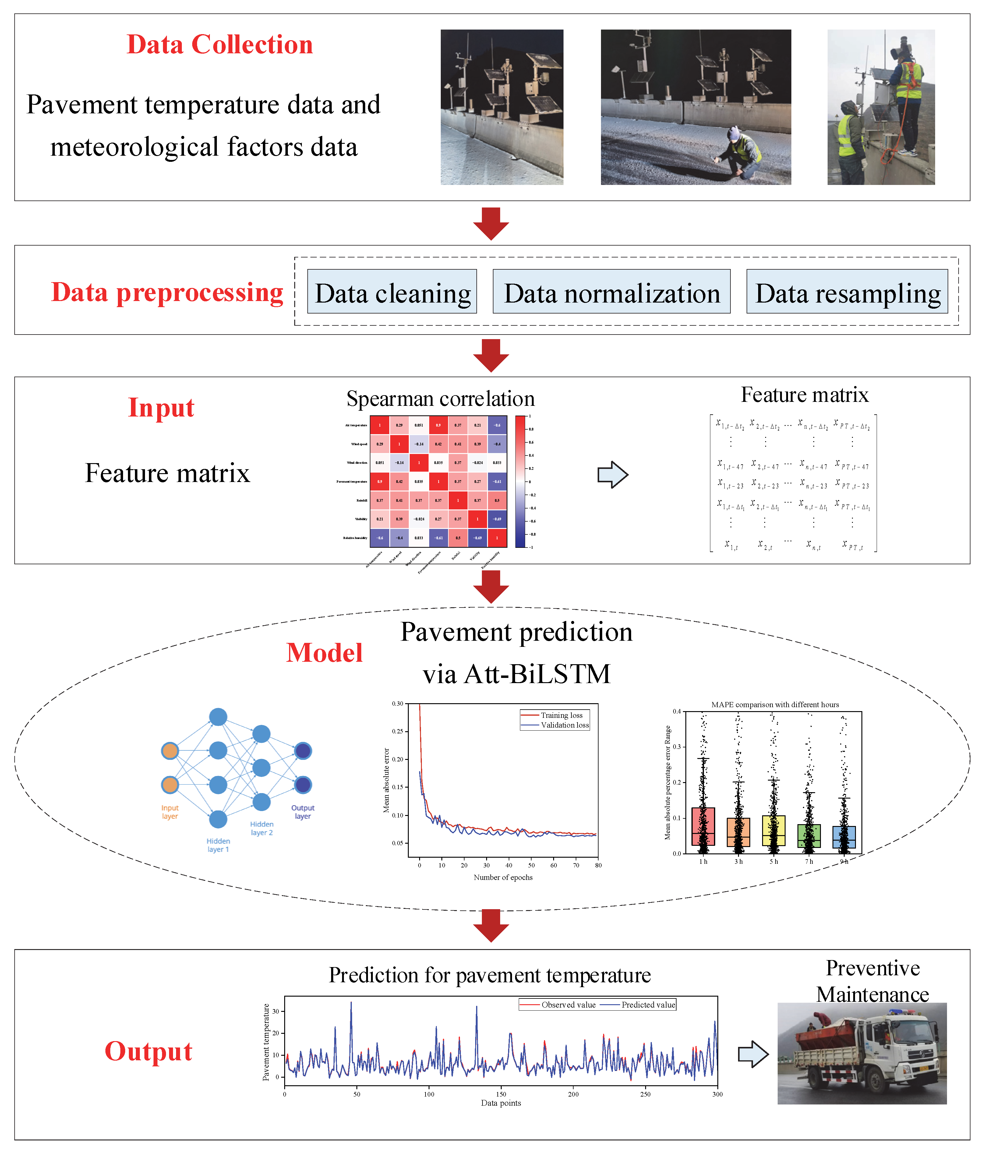
Figure 1 provides the general outline of the research, which consisted of three main steps. (1) The first step was the collection and preprocessing of winter pavement temperature data and meteorological element data. In order to collect accurate data, several road weather stations were installed and checked regularly to ensure the stations worked well. To further improve the data quality, data preprocessing was conducted. (2) The second step determined the model inputs by Spearman correlation coefficients. The input feature matrix had a significant impact on the model, and important variable extraction was performed in order to capture the influence of meteorological factors on pavement temperature and pavement temperature time series characteristics. (3) The third step established the optimal pavement temperature prediction model by adjusting the model hyperparameters to predict the future pavement temperature. The hyperparameters controlled the performance of the model, and in order to obtain the optimal model, the optimal values of parameters such as the size of the sliding window, the number of hidden layer neurons, and the optimizer were obtained through the experiment. Finally, the established attention-based BiLSTM model was used for pavement temperature prediction to further support preventive maintenance.

4. Data

4.1. Data Description

Compared to northern China, southern China receives less snow. When the temperature is low, thin ice is easily created on the road. Thin ice, being smooth and transparent, prevents drivers from observing it and slowing down in advance. Most drivers in Yunnan lack experience in driving in ice and snow, and when they find that the vehicle is out of control, they cannot handle it rationally. As a result, thin ice causes casualties in Yunnan every year.

The observing station is on the Niujiagou bridge on the Maliuwan–Zhaotong line (103°76′13″, 27°74′04″) in the Wumeng Mountains. The raw data are real-time data collected by VAISALA automatic road weather stations every minute, including the main meteorological factors such as pavement temperature, air temperature, humidity, wind speed, and rainfall. An example of the raw data is shown in

Table 1. The raw data format of VAISALA road weather station.

Time	Visibility/m	Temperature/°C	Related Humidity/%	Rainfall/mm	Wind Speed/m/s	Wind Direction/°	Pavement Temperature °C
1 December 2019 0:00	20,000	3.7	92	0	2.3	54	3.7
1 December 2019 0:01	20,000	3.7	93	0	2	32	3.7
…	…	…	…	…	…	…	…

.

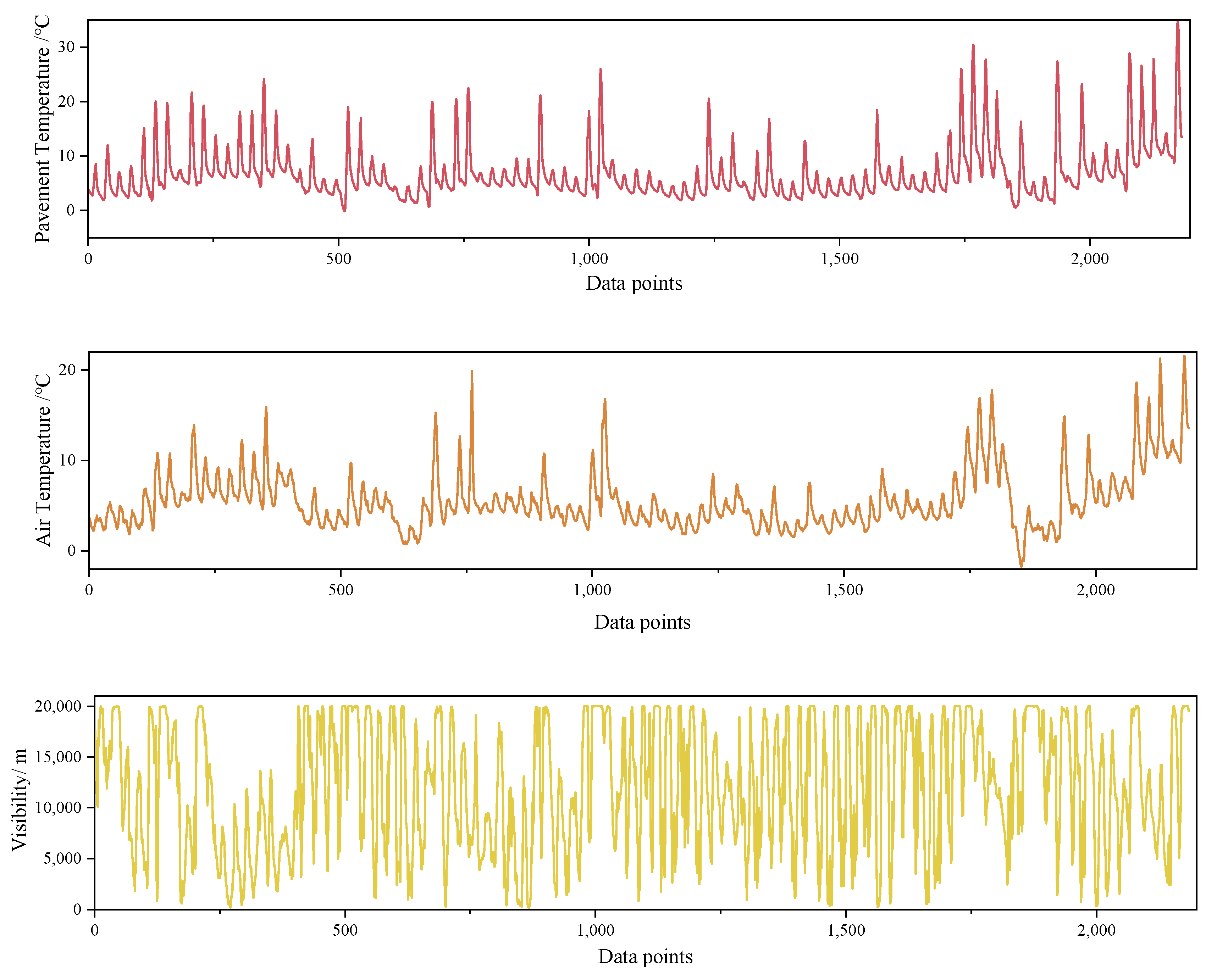
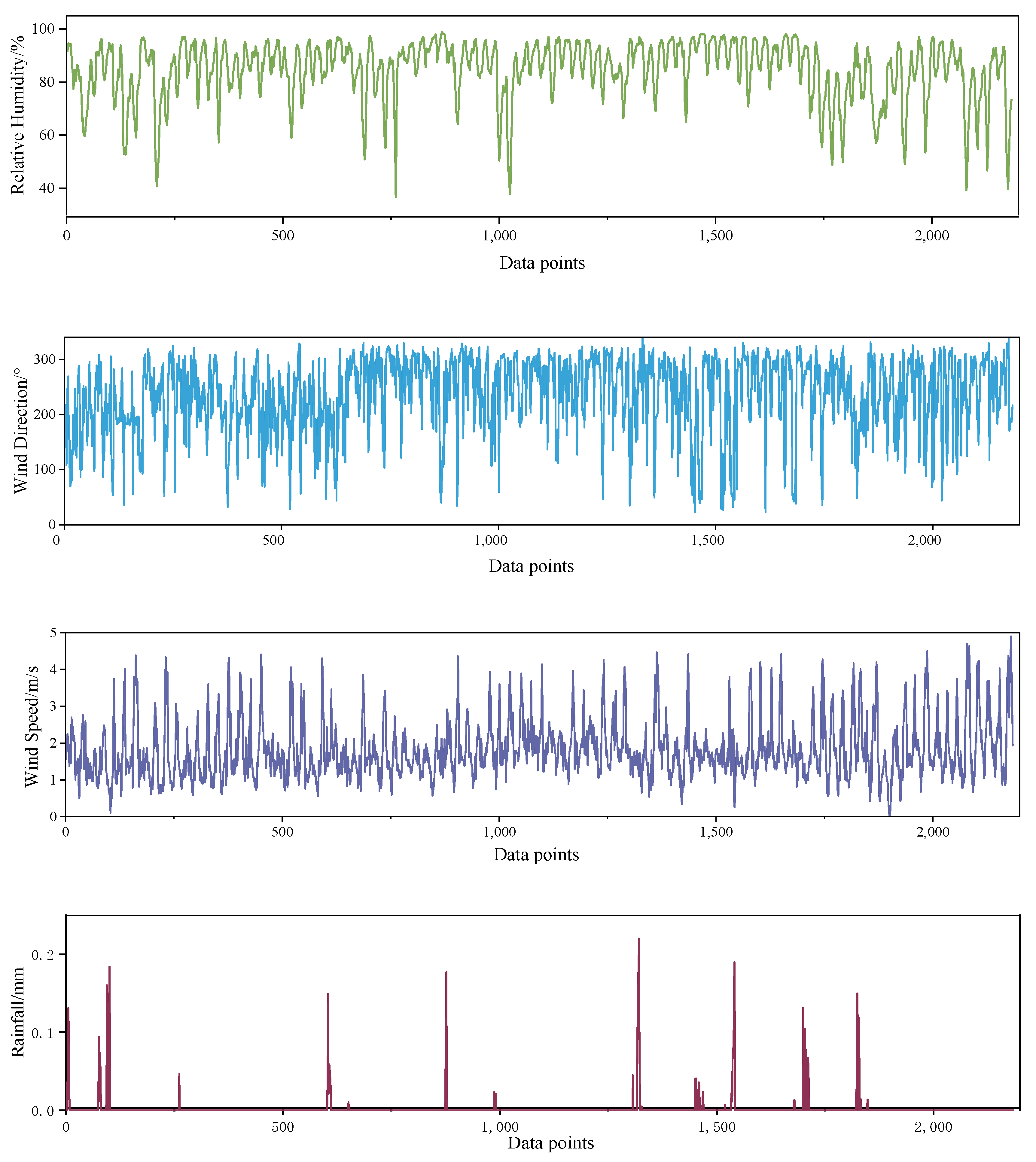
The total data collection period included two time periods from November 2019 to March 2020 and November 2020 to March 2021. Figure 2 shows the time sequence distribution diagrams. After eliminating duplicate, missing, and abnormal data, the data were resampled at the interval of one hour. Thereby, 4344 samples remained for modeling. Figure 2 shows the time sequence distribution diagrams for November 2019 to March 2020. The descriptive statistics of the climatic data and pavement temperature data are presented in

Table 2. Descriptive statistics of the climatic data and pavement temperature data.

Variable	Mean	St. Dev	Max	Min
Visibility	11,110.0	5994.4	20,000.0	112.8
Air temperature	5.4	3.7	22.3	−2.1
Humidity	83.7	11.9	98.9	34.6
Rainfall	0.0	0.0	0.2	0.0
Wind speed	1.8	0.8	5.0	0.0
Wind direction	218.2	75.2	351.3	10.1
Pavement temperature	6.5	5.3	35.9	−4.1

.

The results of the analysis show that the average winter air temperature is about 5.4 degrees Celsius, and the lowest pavement temperature is about −4.1 degrees Celsius. At the same time, the average relative humidity is 83.7% due to the high vegetation cover. Figure 2 shows that the air and pavement temperatures are specifically cyclical.

4.2. Data Preprocessing

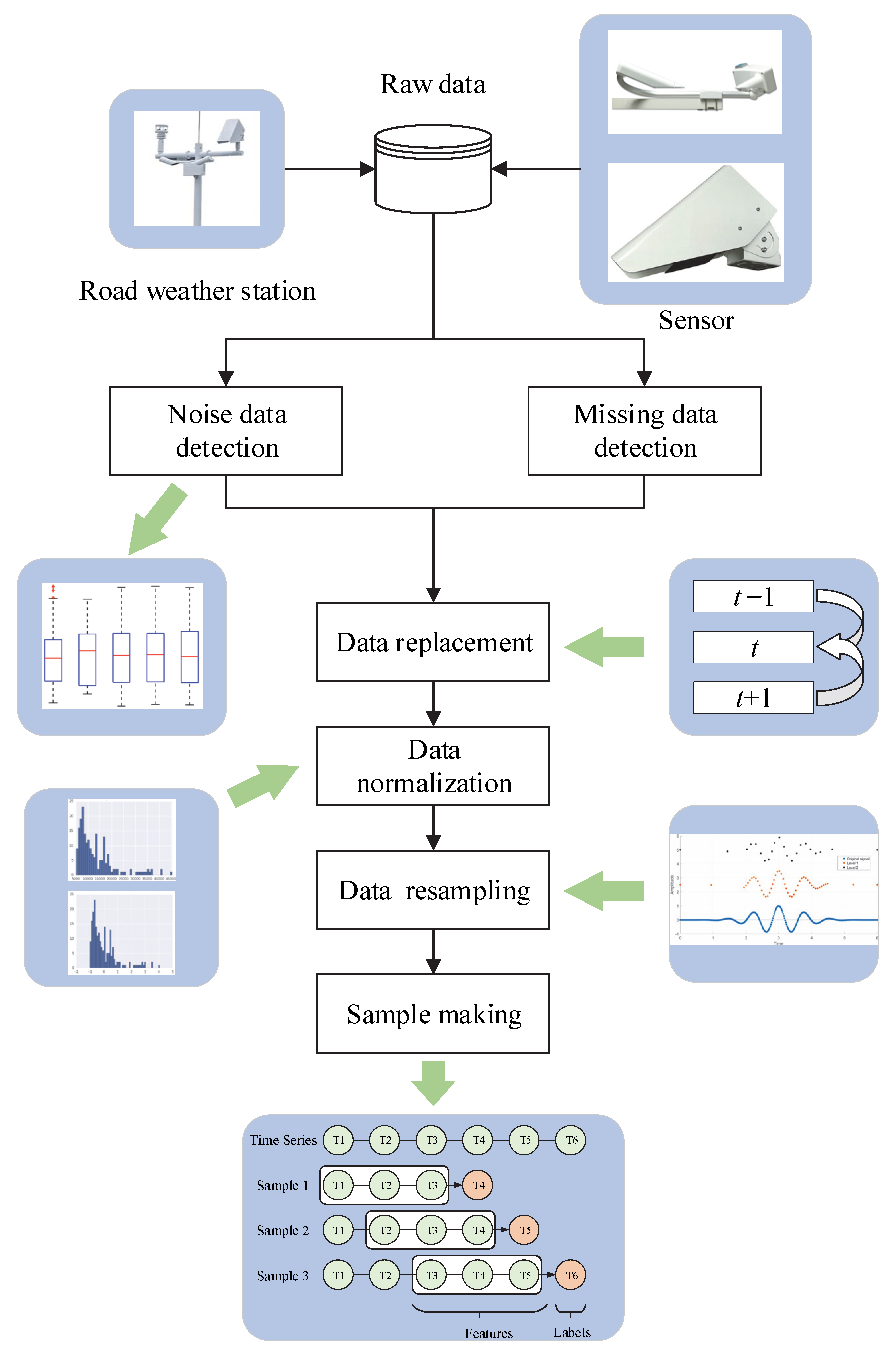
There are many uncontrollable factors in the road weather station data collection process, especially unexpected factors such as vehicle movement and equipment failure, which can lead to missing values and noisy data in the raw data. Therefore, the data processing flow, as shown in Figure 3, was designed, which will be discussed later.

4.2.1. Data Cleaning and Replacement

The three-sigma guidelines were used to identify noisy data, which were considered noisy if the absolute value of the difference between the value and the mean was greater than three times its standard deviation.

$$\left|X_{\mathrm{i}}-\overline{X}\right|>3{\sigma }_X$$

(1)

where $X_{\mathrm{i}}$ is the observed value of the feature; $\overline{X}$ is the mean value of the feature; ${\sigma }_X$ is the standard deviation of the feature.

In this way, noisy data could be detected, and missing values could be found directly from the data. After completing the noisy data and missing data detection, we removed them and filled in the proper data. Due to the high frequency of data collection, we used the average value for filling. The calculation formula is as shown in Equation (2).

$$X_i{}^{\prime }=\frac{X_{i-1}+X_{i+1}}{2}$$

(2)

where $X_i{}^{\prime }$ is the value calculated by the averaging method.

4.2.2. Data Normalization and Resampling

In order to improve the training speed of the model and reduce the impact of different magnitudes between different features on the complexity, the z-score normalization was chosen to linearly transform the original data. The calculation formula is as shown in Equation (3).

$${\widehat{X}}_i=\frac{X_i-\overline{X}}{{\sigma }_X}$$

(3)

where ${\widehat{X}}_i$ is the normalized data.

It was considered that the model could not provide a reference for the prevention of pavement icing if the prediction time interval was too small. Therefore, the minute-Scale data set was resampled at 1 h intervals to form a new data set.

4.2.3. Generating Samples Making

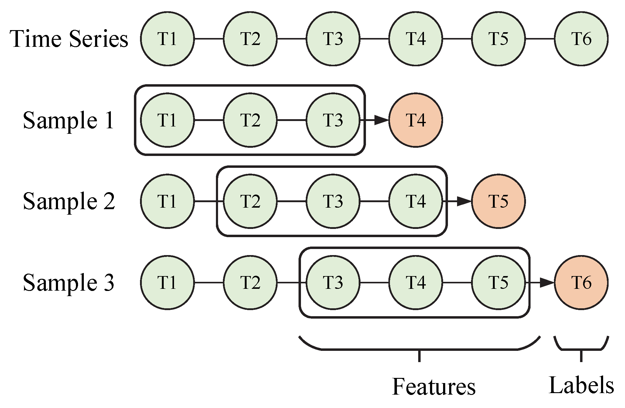
In this paper, the prediction of pavement temperature was considered as a time series problem, which means that the model used the sliding window approach to construct supervised learning samples. As shown in Figure 4, green represents ordinary time series data, time series framed by black lines are used as features, and orange time series represent labels. The process of the sliding window approach is as follows:

(1)

Suppose the number of the sliding window is set as $\Delta t$, which means the model uses the data in the previous times $\left[t-\Delta t,t\right)$ to predict the pavement temperature in time t.

(2)

If the number of time series data is d, a total of $d-\Delta t$ samples can be constructed.

5. Attention-Based BiLSTM Modeling

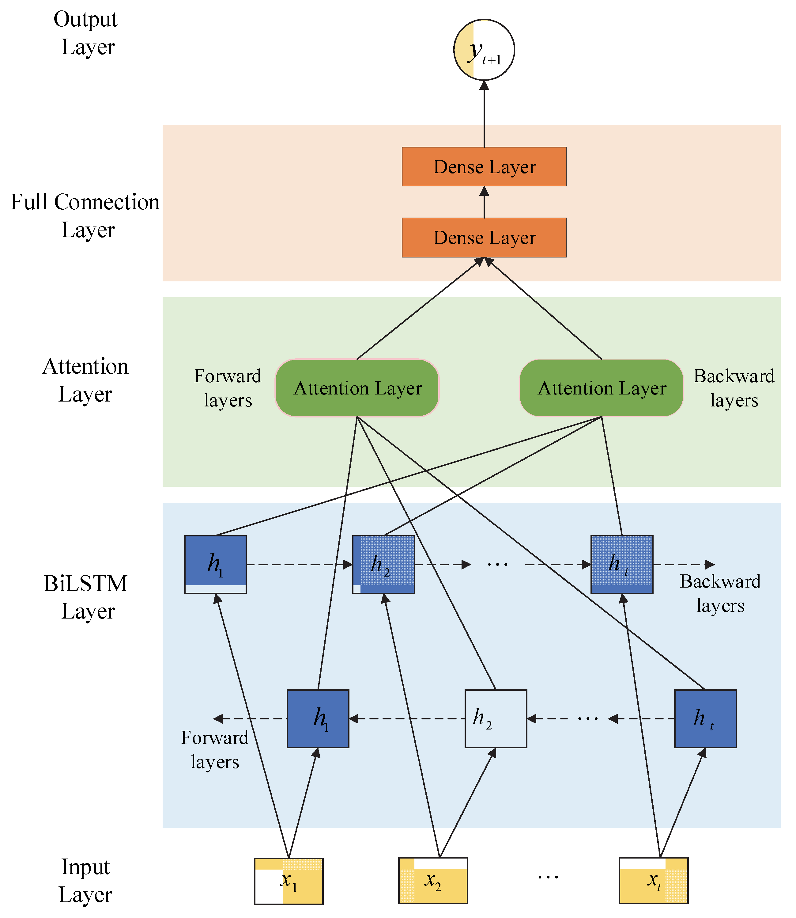
In this paper, an attention-based BiLSTM deep learning model for pavement temperature prediction was proposed. The model consists of five parts: an input layer, BiLSTM layer, attention layer, fully connected layer, and output layer. Figure 5 illustrates the overall architecture of the Att-BiLSTM model. The BiLSTM layer is capable of extracting features from the front and back directions of the pavement temperature time series data. After that, the important features are further extracted using the attention layer to form a new feature vector. The attention mechanism was introduced mainly to optimize the LSTM structure to compensate for its lack of ability to give different levels of attention to features over multiple time steps. Finally, the attention layer is followed by the fully connected (FC) layers, which are regression layers used to make predictions. Each module will be described in detail in the following subsections.

5.1. BiLSTM

Pavement temperatures are affected by the cumulative effect of pavement temperatures at multiple historical moments. When extracting temporal features, the influence of pavement temperature at multiple historical moments should be considered. Recurrent neural networks (RNNs) are a classical architecture for time sequence data prediction, proposed by Hopfield [19]. 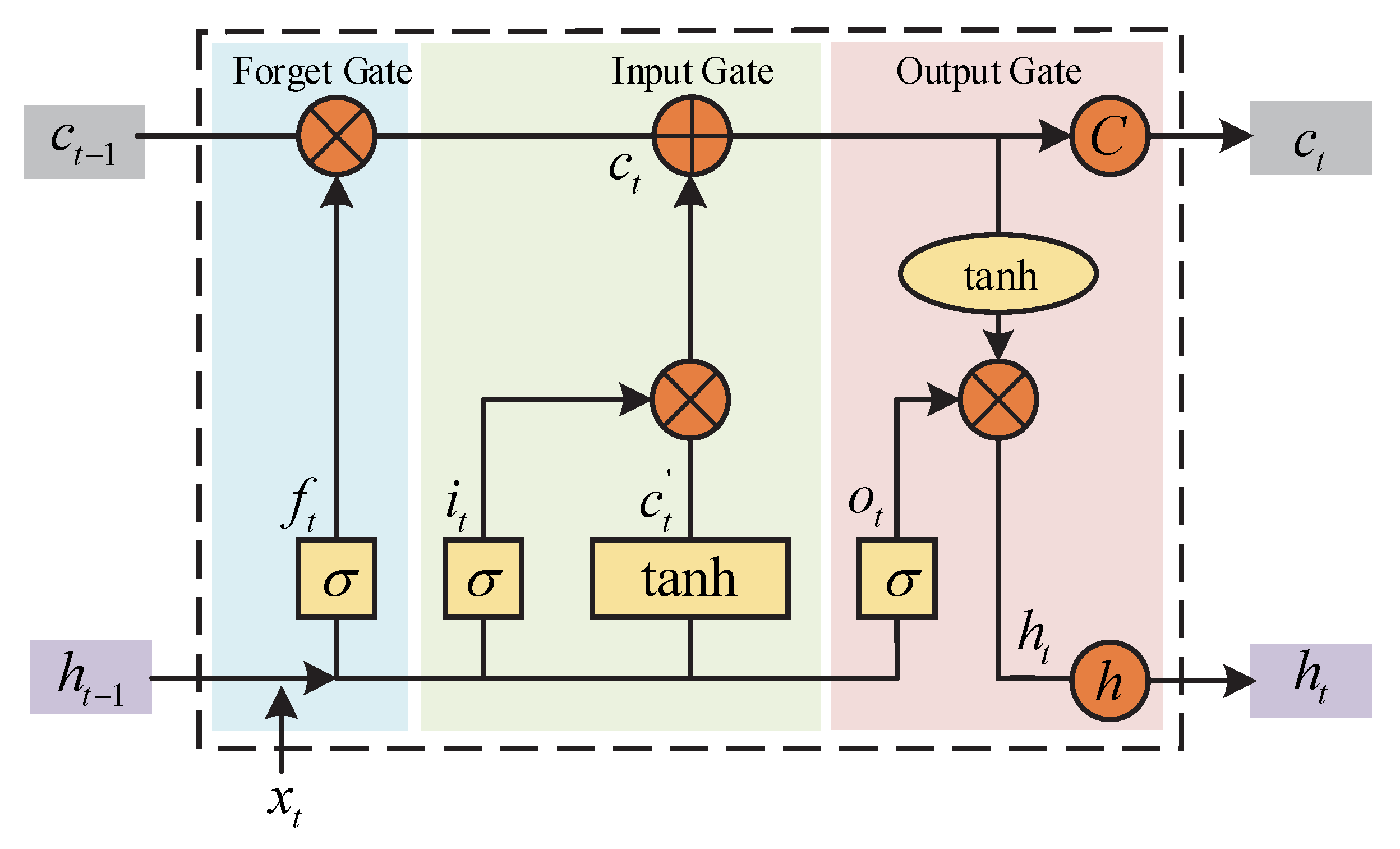The advantage of RNNs is the use of output as feedback in RNNs compared to traditional artificial neural networks, which makes RNNs more effective in learning time-dependence [20]. However, when handling problems with long-term dependencies, RNNs may fail to converge. In order to solve this problem, Hochreiter and Schmidhuber proposed a long-short-term memory (LSTM) neural network, which introduces memory cells to deal with long-term dependencies [21]. The LSTM neural network is shown in Figure 6.

With the help of the LSTM neural network, the temporal characteristics of the actual values at the predicted target moment can be extracted from the actual pavement temperature sequence at the target window moment and only mapped to the actual pavement temperature at the target prediction moment, enabling prediction on a time series scale. The LSTM network is calculated as follows:

$$f_t=\sigma (W_f\cdot [h_{t-1},x_t]+b_f)$$

(4)

$$i_t=\sigma (W_i\cdot [h_{t-1},x_t]+b_i)$$

(5)

$$c_t^{\prime }=\tanh (W_C\cdot [h_{t-1},x_t]+b_C)$$

(6)

$$c_t=f_t\cdot c_{t-1}+i_t\cdot c_t^{\prime }$$

(7)

$$o_t=\sigma (W_o\cdot [h_{t-1},x_t]+b_o)$$

(8)

$$h_t=o_t\cdot \tanh (c_t)$$

(9)

where $t$ is the moment; $x_t$ is the current moment input; $f_t$ is forget gate; $i_t$ is input gate; $c_t^{\prime }$ is a temporary cell state; $c_t$ is a cell state; $o_t$ is output gate; $h_t$ is the output of the hidden layer at the current moment; $c_{t-1}$ is the state of the cell at the previous moment; $h_{t-1}$ is the output of the hidden layer at the previous moment; $W_f$, $W_i$, $W_C$, $W_o$ are the weights to be learned, respectively; $b_f$, $b_i$, $b_C$, $b_o$ are the offsets to be learned; $\sigma$ is the $sigmoid$ activation function.

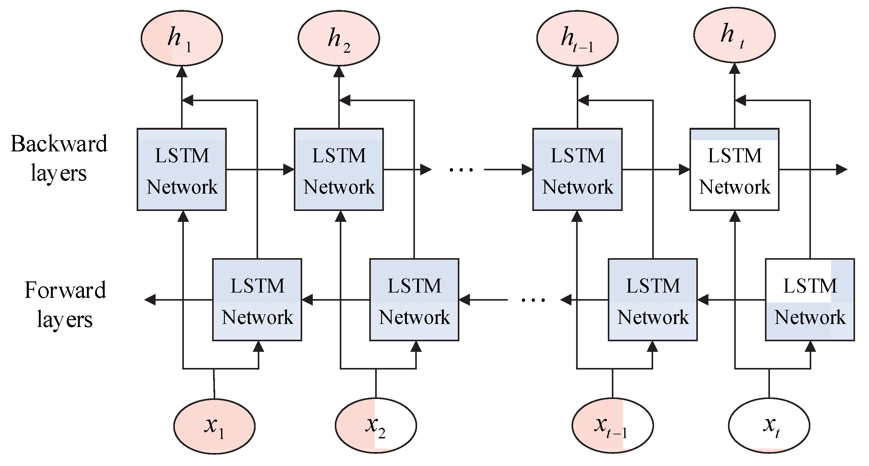
Although LSTM overcomes the limitations of RNNs, it can still only process sequence information from the past and cannot utilize front sequence information. Huang et al. [22] proposed a bidirectional LSTM (BiLSTM) including forward and backward LSTM layers, as shown in Figure 7. A BiLSTM is able to integrate and process information from both the front and rear, capturing road temperature and associated parameter time information more effectively.

5.2. Attention Mechanism

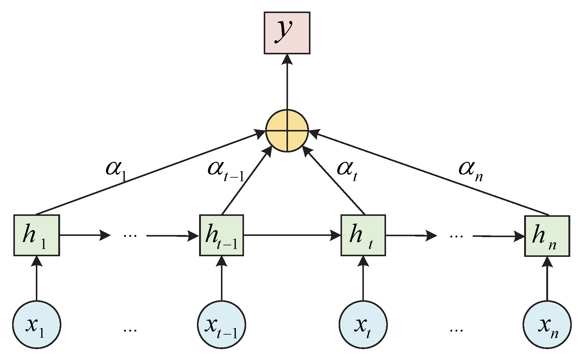
The attention mechanism is a distribution mechanism inspired by the human brain. The human brain focuses on the area that needs to be focused, reducing or even not giving attention to other areas to obtain more important detailed information. In other words, the attention mechanism gives higher weights to relevant parts while minimizing irrelevant parts by giving them lower weights, thus improving the accuracy of the model. The attention mechanism structure is shown in Figure 8.

Here, $x_t(t\in [1,n])$ denotes the input to the BiLSTM network, $h_t(t\in [1,n])$ is the output of the hidden layer obtained by BiLSTM for each input, ${\alpha }_t(t\in [1,n])$ is the output of the attention mechanism for the BiLSTM hidden layer attention probability distribution, and $y$ is the output value of the BiLSTM with the introduction of the attention mechanism.

5.3. Evaluation Metric

Several common performance metrics are used to evaluate the performance of the model: mean absolute error (MAE), mean square error (MSE), and mean absolute percentage error (MAPE), which are calculated using (10)–(12).

$$MAE=\frac{{\displaystyle {\sum }_{\mathrm{i}=1}^N\left|y_i-{\widehat{y}}_i\right|}}{N}$$

(10)

$$MSE=\frac{{{\displaystyle {\sum }_{n=1}^N(y_i-{\widehat{y}}_i)}}^2}{N}$$

(11)

$$MAPE=\frac{100\%}{N}{\displaystyle {\sum }_{i=1}^N\left|\frac{y_i-{\widehat{y}}_i}{y_i}\right|}$$

(12)

where $y_i$ represents the observed pavement temperature and ${\widehat{y}}_i$ represents the predicted pavement temperature.

6. Results and Discussion

6.1. Selection of Important Characteristic Variables

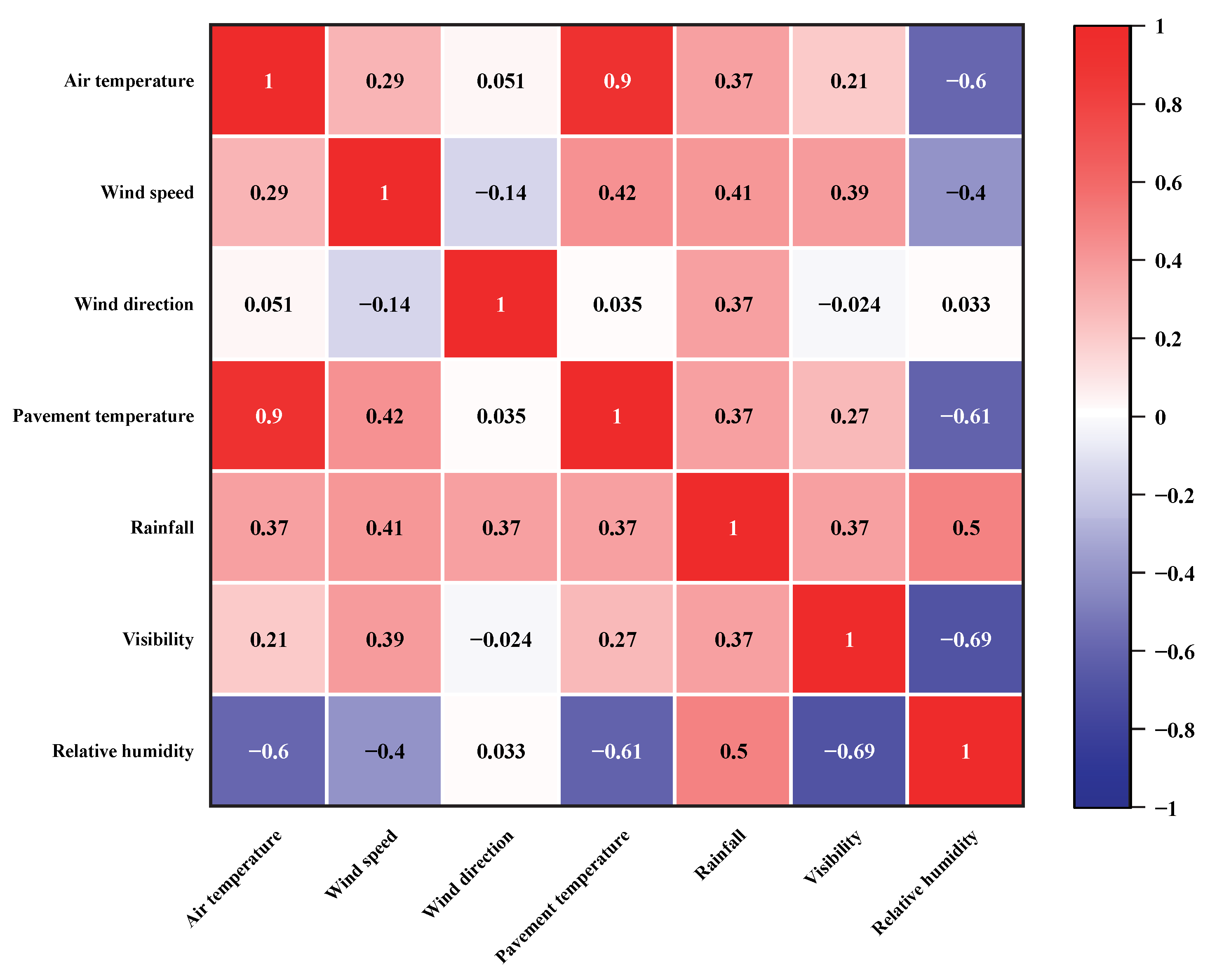
We aimed to reduce the complexity of the model input and improve the accuracy of the prediction model. The characteristic variables with significant correlation with the predicted target value of the pavement temperature were used as the input variables of the pavement temperature prediction model. Considering the possible nonlinear correlation between meteorological characteristics and pavement temperature, a Spearman correlation analysis was performed for the six meteorological characteristics variables as well as pavement temperature. The Spearman’s rank correlation coefficient method is often used to analyze the closeness of a relationship between two variables and is calculated as:

$$r=\frac{{\displaystyle {\sum }_{i=1}^n(f_i-\overline{f_i})}(f_j-\overline{f_j})}{\sqrt{{\displaystyle \sum {}_{i=1}^n}{(f_i-\overline{f_i})}^2{\displaystyle \sum {}_{i=1}^n}{(f_j-\overline{f_j})}^2}}$$

(13)

where $\overline{f_i}$ and $\overline{f_j}$ are the mean of the experimental values $f_i$ and $f_j$, respectively, $r$ is the Spearman rank correlation coefficient, and the closer $\left|r\right|$ is to 1, the higher the degree of linear correlation between $f_i$ and $f_j$. The results are shown in Figure 9.

The correlation coefficient between air temperature and pavement temperature was 0.9, indicating an extremely strong correlation between air temperature and road surface temperature. The correlation coefficients between wind speed, rainfall, visibility, and relative humidity were weakly correlated with pavement temperature, with correlation coefficients of 0.42, 0.37, 0.37, and −0.61, respectively. The correlation coefficient between wind direction and pavement temperature was 0.035, indicating a very weak correlation between wind direction and pavement temperature. Based on the Spearman correlation coefficient results, air temperature, wind speed, rainfall, relative humidity, and previous road surface temperature were selected as input features.

6.2. Optimal Parameters of the Att-BiLSTM Model

After building the model structure and determining the input features of the model, the next step was the training of the model. We divided the dataset into a ratio of 70% for the training set, 20% for the test set, and 10% for the validation set. The Keras application programming interface for TensorFlow was chosen to implement the model proposed in this paper. For the proposed model, there are several important parameters that have a significant impact on the prediction performance, including the size of the sliding window, the number of hidden layer neurons, the type of optimizer, and the number of training epochs. The grid search cross-validation method is used to find the optimal hyperparameters. The optimization process for these parameters is shown below.

6.2.1. The Size of Sliding Window

For time sequence data, the size of the sliding window is the most important parameter, as it directly affects the input features and the number of samples. Inputting sequences with high time correlation into the model can effectively improve the prediction accuracy of the model, while inputting sequences with low time correlation into the model will add irrelevant information. Considering the thermal inertia of the pavement temperature, the size of the sliding window was set to 1 h, 3 h, 5 h, 7 h, and 9 h, respectively. These values were tested, and the optimal value was selected by the evaluation metric.

The results of the calculations are shown in

Table 3. Performance of the models when the size of the sliding window is 1 h, 3 h, 5 h, 7 h, and 9 h.

$\Delta \mathit{t}/$h	MAE	MSE	MAPE
1 h	0.662	1.678	0.120
3 h	0.419	0.531	0.138
5 h	0.457	0.890	0.196
7 h	0.334	0.353	0.101
9 h	0.345	0.387	0.115

and Figure 10, which indicate that when the size of the sliding window was 7 h, the prediction performance of the model proposed was the best.

6.2.2. The Number of Hidden Layer Neurons

For neural networks, the number of hidden layer neurons also plays a significant role. Too few hidden layer neurons can lead to underfitting of the model and the inability to predict accurately, while too many can lead to overfitting and also increase the time complexity. The search space was set at 50 to 300.

As can be seen from

Table 4. Performance of the model with the different number of neurons.

The Number of Neurons	MAE	MSE	MAPE
50	0.391	0.389	0.239
100	0.368	0.392	0.178
150	0.334	0.353	0.101
200	0.393	0.430	0.164
250	0.398	0.434	0.189
300	0.430	0.454	0.239

, when the number of neurons was 150, the prediction performance of the model proposed was the best.

6.2.3. The Optimizer

During the model training process, the model parameters were adjusted and changed to obtain the minimum loss function. The role of the optimizer is to guide the loss function to update in the right direction. In this paper, four commonly used optimizers are compared: Adaptive Moment Estimation (Adam), Stochastic gradient descent (SGD), Adaptive Gradients (Adagrad), and Root Mean Square Prop (RMSprop).

As can be seen from

Table 5. Performance of the models when the optimizer is Adam, SGD, Adagrad, or RMSprop.

Optimizer	MAE	MSE	MAPE
Adam	0.334	0.353	0.101
SGD	1.329	3.363	1.001
Adagrad	1.187	4.376	0.329
RMSprop	0.367	0.379	0.204

, when the optimizer was Adam, the prediction performance of the model proposed was the best.

6.2.4. The Training Epochs

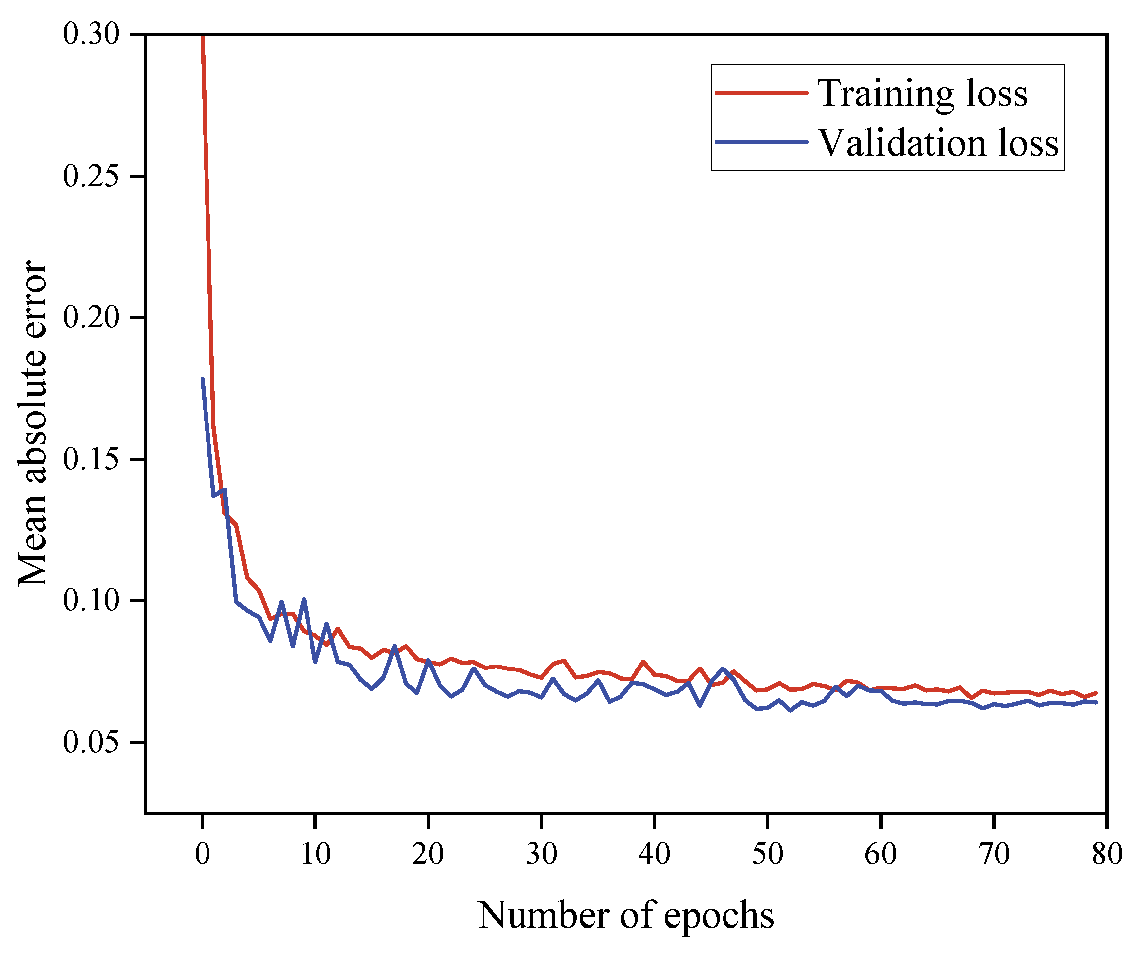
Figure 11 shows the prediction performance of the model in the training and validation sets, through which the performance of the model on the training and validation data can be evaluated to obtain the best epochs and prevent the model from overfitting or underfitting. It can find that in terms of training and validation data, the MAE gradually decreases as the epoch increases, which indicates that the model accuracy improves. The validation loss of the model is mostly lower than the training loss, and when the epoch is roughly 70, both the training loss and validation loss tend to be smooth, which suggests that the optimal epochs are around 70.

6.3. Performance Comparison

In this section, the predictive performance of the model proposed in the study is compared with that of other deep learning methods, including RNNs, GRU networks, LSTM networks and BiLSTM networks. The proposed Att-BiLSTM model and other baseline models were trained based on the same training data set.

Table 6. Predictive performance comparison of the proposed model with other models.

Algorithm	MAE	MSE	MAPE
RNN	0.460	0.544	0.184
GRU	0.445	0.491	0.170
LSTM	0.428	0.515	0.165
BiLSTM	0.386	0.437	0.140

shows the prediction performance comparison of the LSTM with other baseline models. The results show that RNNs have the largest prediction error among all the algorithms for all three metrics. This is because RNNs directly use the entire output as feedback and cannot forget and update the influence of meteorological factors, which leads to poor prediction. The GRU networks, as a variant of LSTM networks, have the ability to forget and update information. Compared with RNNs, the GRU networks achieved better prediction performance, where MAE, MSE, and MAPE were reduced by 3.2%, 9.7%, and 7.6% on average, respectively. However, the GRU network still falls short of the LSTM networks in terms of prediction performance due to its simplified cell states. Compared to the above two methods, the LSTM networks further improve the prediction performance, but the effective prediction of pavement temperature not only relies on past information but also considers the time sequence. The BiLSTM networks can integrate and process data from both front and back directions, which can solve the problem that LSTM only follows a one-way sequential order in information processing and can effectively capture the time sequence information of pavement temperature to achieve better prediction. The proposed model in this paper, by introducing the attention mechanism, adaptively calculates and adjusts the hidden layer state values corresponding to the original input features to highlight the important features and weaken the minor features to further explore the internal characteristics of the pavement temperature data. 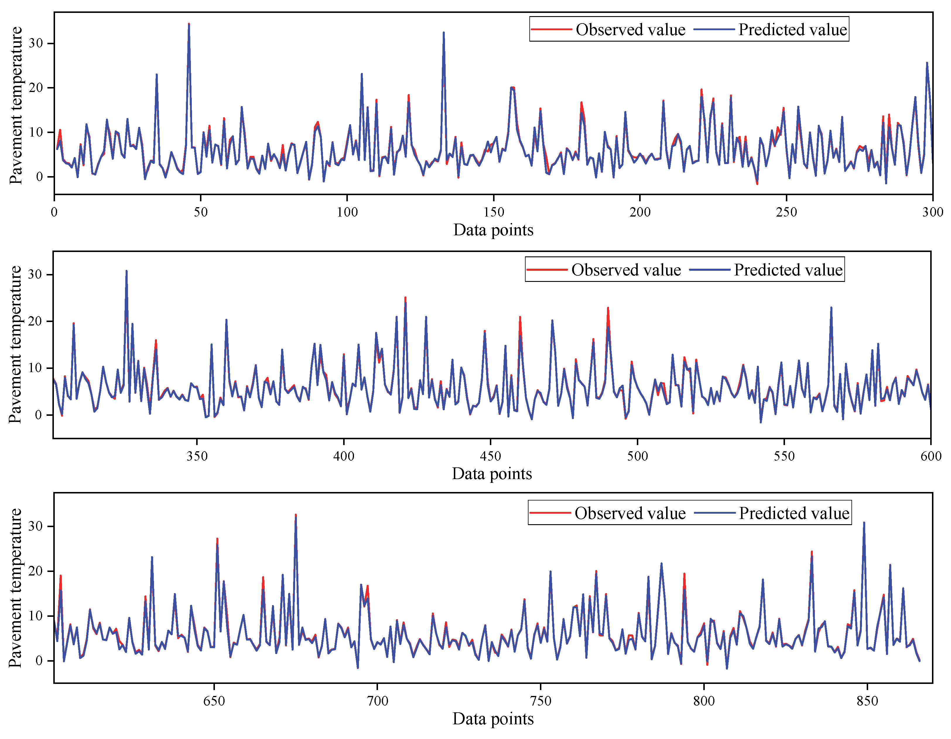Therefore, the proposed model outperformed all models with the MAE of 0.334, MSE of 0.353, and MAPE of 10.1%. The comparison of pavement temperature truth and the predicted values of the proposed model on multiple days is visualized in Figure 12.

6.4. Discussion

In this section, the prediction results and applications of the proposed model are analyzed and discussed.

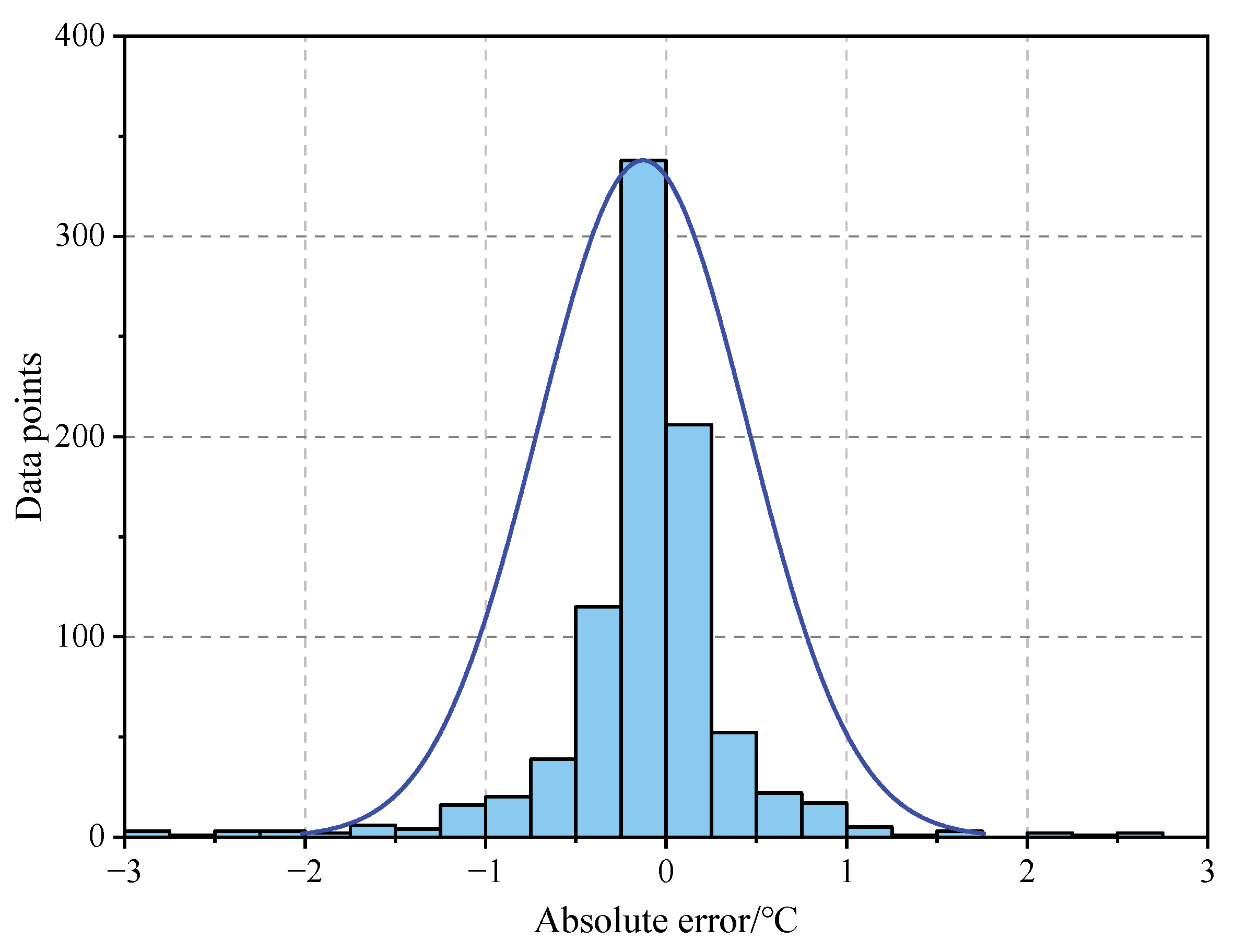
Figure 13 shows the absolute errors of the predicted values of the proposed model and observed values. It can be seen that 93.4% of the absolute error is less than 1 °C, and 82.1% of the absolute error is less than 0.5 °C, which indicates that the model has a good predictive effect.

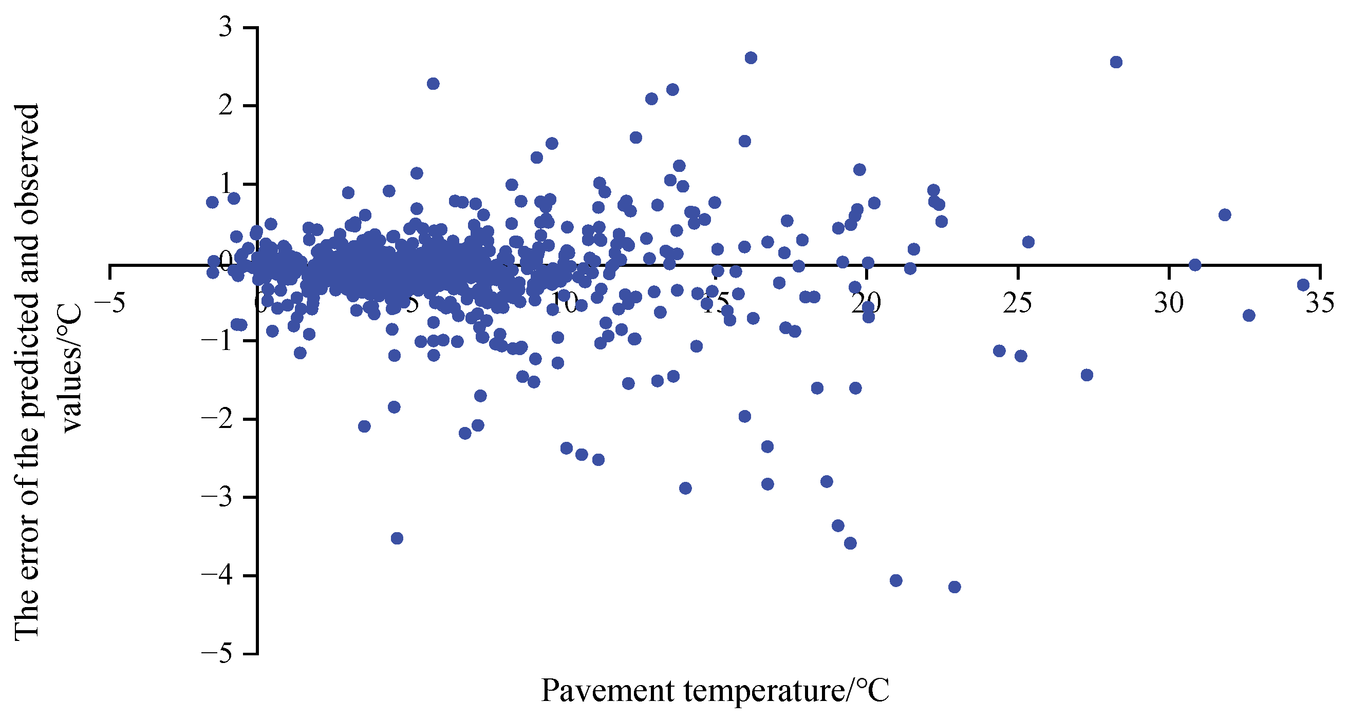
From Figure 14, it can be found that the error values of the prediction model are more concentrated in low temperatures (−5 to 5 °C), which are prone to icing, and almost all of them are less than 1 °C. The prediction performance of the model in the high-temperature is weakened and is not as good as that in the low-temperature segment, with a more discrete distribution of error values. This may be due to the greater influence of meteorological elements such as solar radiation and total cloudiness on the road surface temperature in the high-temperature condition, which leads to fluctuations in the prediction errors. Overall, the Att-BiLSTM model has better performance in the low-temperature condition and has good prospects for engineering applications in winter low-temperature pavement temperature prediction.

The Att-BiLSTM pavement temperature prediction model proposed in this work can be combined with the pavement icing formation mechanism to determine future pavement icing and improve the accuracy and reliability of icing warning. Together with the facilities such as variable information boards or speed limit signs near the point (section), timely information on dangerous road conditions of bad driving conditions (or early warnings of road surface icing points) can be released to drivers, prompting them to control speed and drive carefully, thus reducing the occurrence of vicious traffic accidents such as vehicle skidding and rollover or rear-end collision.

7. Conclusions

The prediction of a pavement temperature at the microscopic scale has been a challenge to be solved. To address this problem, an Att-BiLSTM pavement temperature prediction model based on historical meteorological data and pavement temperature data was developed in this study. Pavement temperature data and meteorological data collected from road weather stations on route G85 from Maliuwan to Zhaotong in Yunnan, China, which covered 180 days. A feature vector was constructed to describe the influence of meteorological features on pavement temperature and the time series characteristics of pavement temperature by Spearman’s correlation coefficient analysis. The Att-BiLSTM model predicted the future pavement temperature based on the feature vector. To demonstrate the validity of the model, RNNs, GRU, LSTM and BiLSTM networks were selected as benchmark models to compare their prediction performance with the prediction performance of the proposed model. The results show that the MAE, MSE, and MAPE of the proposed Att-BiLSTM model were 0.330, 0.339, and 10.1%, respectively, which were better than the other baseline models. It was shown that 93.4% of the predicted values had an error less than 1 °C, and 82.1% had an error less than 0.5 °C, indicating that the proposed model has a great prediction performance. The proposed prediction model has better performance at low temperatures (−5~5 °C). This shows that the method proposed in this paper has good prospects for engineering applications in low-temperature pavement temperature prediction in winter.

In future work, internal pavement or subgrade temperatures should be further considered to obtain better performance within the pavement temperature prediction model. In addition, the pavement temperature prediction model should be combined with the pavement temperature prediction model to further predict pavement conditions.

References

- Chen, S.; Saeed, T.U.; Labi, S. Impact of road-surface condition on rural highway safety: A multivariate random parameters negative binomial approach. Anal. Methods Accid. Res. 2017, 16, 75–89. [Google Scholar] [CrossRef]
- Strong, C.K.; Ye, Z.; Shi, X. Safety effects of winter weather: The state of knowledge and remaining challenges. Transp. Rev. 2010, 30, 677–699. [Google Scholar] [CrossRef]
- Chen, J.; Wang, H.; Xie, P. Pavement temperature prediction: Theoretical models and critical affecting factors. Appl. Therm. Eng. 2019, 158, 113755. [Google Scholar] [CrossRef]
- Zapata, C.E.; Andrei, D.; Witczak, M.W.; Houston, W. Incorporation of environmental effects in pavement design. Road Mater. Pavement Des. 2007, 8, 667–693. [Google Scholar] [CrossRef]
- Lei, D.; Liu, H.; Le, H.; Huang, J.; Yuan, J.; Li, L.; Wang, Y. Ionospheric TEC Prediction Base on Attentional BiGRU. Atmosphere 2022, 13, 1039. [Google Scholar] [CrossRef]
- Sass, B.H. A numerical model for prediction of road temperature and ice. J. Appl. Meteorol. Climatol. 1992, 31, 1499–1506. [Google Scholar] [CrossRef]
- Voldborg, H. On the prediction of road conditions by a combined road layer-atmospheric model in winter. Transp. Res. Rec. 1993, 1387, 231. [Google Scholar]
- Meng, C. A numerical forecast model for road meteorology. Meteorol. Atmos. Phys. 2018, 130, 485–498. [Google Scholar] [CrossRef]
- Chen, J.; Li, L.; Wang, H. Analytical prediction and field validation of transient temperature field in asphalt pavements. J. Cent. South Univ. 2015, 22, 4872–4881. [Google Scholar] [CrossRef]
- Karsisto, V.; Nurmi, P. Using car observations in road weather forecasting. In Proceedings of the International Road Weather Conference, Fort Collins, CO, USA, 27–29 April 2016; Available online: https://www.researchgate.net/profile/Virve-Karsisto/publication/306099501_Using_car_observations_in_road_weather_forecasting/links/57b1524c08ae95f9d8f3bbb2/Using-car-observations-in-road-weather-forecasting.pdf (accessed on 1 August 2022).
- Park, J.J.; Shin, E.C.; Yoon, B.J. Development of frost penetration depth prediction model using field temperature data of asphalt pavement. Int. J. Offshore Polar Eng. 2016, 26, 341–347. [Google Scholar] [CrossRef]
- Asefzadeh, A.; Hashemian, L.; Bayat, A. Development of statistical temperature prediction models for a test road in Edmonton, Alberta, Canada. Int. J. Pavement Res. Technol. 2017, 10, 369–382. [Google Scholar] [CrossRef]
- Kršmanc, R.; Slak, A.Š.; Demšar, J. Statistical approach for forecasting road surface temperature. Meteorol. Appl. 2013, 20, 439–446. [Google Scholar] [CrossRef]
- Gedafa, D.S.; Hossain, M.; Romanoschi, S.A. Perpetual pavement temperature prediction model. Road Mater. Pavement Des. 2014, 15, 55–65. [Google Scholar] [CrossRef]
- Yang, C.H.; Yun, D.G.; Kim, J.G.; Lee, G.; Kim, S.B. Machine learning approaches to estimate road surface temperature variation along road section in real-time for winter operation. Int. J. Intell. Transp. Syst. Res. 2020, 18, 343–355. [Google Scholar] [CrossRef]
- Molavi Nojumi, M.; Huang, Y.; Hashemian, L.; Bayat, A. Application of machine learning for temperature prediction in a test road in Alberta. Int. J. Pavement Res. Technol. 2022, 15, 303–319. [Google Scholar] [CrossRef]
- Milad, A.; Adwan, I.; Majeed, S.A.; Yusoff, N.I.M.; Al-Ansari, N.; Yaseen, Z.M. Emerging technologies of deep learning models development for pavement temperature prediction. IEEE Access 2021, 9, 23840–23849. [Google Scholar] [CrossRef]
- Li, Y.; Chen, J.; Dan, H.; Wang, H. Probability prediction of pavement surface low temperature in winter based on bayesian structural time series and neural network. Cold Reg. Sci. Technol. 2022, 194, 103434. [Google Scholar] [CrossRef]
- Hopfield, J.J. Neural networks and physical systems with emergent collective computational abilities. Proc. Natl. Acad. Sci. USA 1982, 79, 2554–2558. [Google Scholar] [CrossRef] [PubMed]
- Wu, X.; Liu, Z.; Yin, L.; Zheng, W.; Song, L.; Tian, J.; Yang, B.; Liu, S. A haze prediction model in chengdu based on LSTM. Atmosphere 2021, 12, 1479. [Google Scholar] [CrossRef]
- Graves, A. Long short-term memory. In Supervised Sequence Labelling with Recurrent Neural Networks; Springer: Berlin/Heidelberg, Germany, 2012; pp. 37–45. [Google Scholar] [CrossRef]
- Huang, Z.; Xu, W.; Yu, K. Bidirectional LSTM-CRF models for sequence tagging. arXiv 2015. [Google Scholar] [CrossRef]
Figure 1.
General outline of the research methodology.
Figure 2.
Distribution of each measured variable. Pavement temperature (first), air temperature (second), visibility (third), relative humidity (fourth), wind direction (fifth), wind speed (sixth) and rainfall (last).
Figure 3.
The data processing flow.
Figure 4.
Sliding window approach.
Figure 5.
Framework of the proposed model.
Figure 6.
Long short-term memory neural network.
Figure 7.
Bidirectional long short-term memory neural network.
Figure 8.
Structure of attention mechanism.
Figure 9.
Correlation coefficients between pavement temperature and various meteorological factors.
Figure 10.
Errors comparison with different hours. MAE (left), MSE (middle), MAPE (right).
Figure 11.
Performance of the model during training and validation error.
Figure 12.
Comparison of pavement temperature truth and predicted values in the test set. Data points 1–300 in the test set (first), Data points 301–600 in the test set (second), Data points 601–866 in the test set (third).
Figure 13.
The error of the predicted and observed values.
Figure 14.
Distribution of errors.