Aerosol Property Analysis Based on Ground-Based Lidar in Sansha, China

Abstract

Marine aerosol is one of the most important natural aerosols. It has a significant impact on marine climate change, biochemical cycling and marine ecosystems. Previous studies on marine aerosols, especially in the South China Sea, were carried out by satellite and shipborne measurements. The above methods have drawbacks, such as low temporal–spatial resolution and signal interference. However, lidar has high accuracy and high temporal–spatial resolution, so it is suitable for high-precision long-term observations. In this work, we obtain marine aerosol data using Mie Lidar in Sansha, an island in the South Chain Sea. Firstly, by comparing boundary layer height (BLH) between Sansha and Hefei, we found that Sansha’s boundary layer height has significant differences with that of inland China. Secondly, we compare the aerosol extinction coefficients and their variation with height in Sansha and Hefei. Finally, we obtain hourly averaged aerosol optical depth at Sansha and explore its relation with weather. To analyze the AOD–weather relation, we select three meteorological factors (sea surface temperature, mean sea level pressure and 10 m u-component of wind) based on their feature importance, which is determined by random forest regression. We also analyze the relationship between AOD and the above meteorological factors in each season separately. The results show that there is a strong relation between the meteorological factors and AOD in spring and summer, while there is no clear correlation in fall and winter. These analyses can provide valid data for future researches on marine aerosols in the South China Sea.

1. Introduction

Aerosols are liquid or solid particles suspended in the atmosphere, with particle sizes ranging from 0.01 μm to 10 μm. Aerosols can be divided into anthropogenic aerosols or natural aerosols. Aerosol components may come from ocean droplets, forest fires, biomass burning [1], volcanic activity, soil ions or pollens. Human activities, such as burning fossil fuels, chemical product processing and ore mining, also emit aerosol particles into the atmosphere. In addition, aerosols can be classified into marine aerosols and continental aerosols. Marine aerosol is an important kind of aerosol that can greatly impact climate change, water cycles [2] and ecosystems [3]. Marine aerosols interact with multiple meteorological factors and influence the atmosphere environment. Firstly, the distribution of marine aerosols can affect radiation balance. Marine aerosols have an extinction effect on solar radiation, i.e., scattering and absorption of solar radiation. Dynamics of radiation balance will change the temperature distribution of atmosphere and ocean water, which further affect atmospheric circulation and sea–air exchange. In addition, marine aerosol can change cloud micro-physical properties. By forming into cloud condensation nuclei (CCN) and ice nuclei (IN), aerosol particles participate in cloud micro-physical processes and rain formation [4]. It is obvious that marine aerosols have a complex impact on the atmospheric environment of marine areas and coastal areas.

Thus, research on marine aerosols is challenging but essential. Some studies focus on the relation between meteorological factors and aerosol properties. Wind direction [5], temperature [6] and relative humidity [7] are closely related to aerosol particles’ formation, transportation and property. Furthermore, studies of meteorology–aerosol relation are important, since they can bring indications to other studies. For example, the study of [8] analyzes the impact of precipitation and ocean convection on the accuracy of global aerosol models. The study of [9] uses MODIS AOD data and meteorological data to estimate PM10 in Malaysia. In addition, from an application perspective, aerosol research can be used in pollutant estimation [10], weather forecast [11] and air pollution prediction [12,13]. Previous studies also link aerosol with climate change, global warming [14,15], carbon cycle [16] and even food cultivation [17].

Satellite [18,19], shipborne measurements [20], airborne measurements [21] and lidar are frequently used to observe marine aerosols. Among the above techniques, lidar has higher accuracy and temporal–spatial resolution. There are many studies related to aerosols and lidar application, such as aerosol property analysis [22], aerosol classification [23], aerosol field measurement [24], lidar ratio selection [25], calculation and data correction for other meteorological parameters [26,27], etc.

Previous studies on marine aerosols in China show that aerosol’s property and distribution vary in different sea area [28,29]. In some areas, aerosol optical thickness changes apparently during different seasons, while in other areas, remains stable. As for the relation between aerosols and meteorological factors, aerosols may have strong dependence on wind speed [30], relative humidity [31] and temperature [32]. What’s more, present studies are mostly carried out in Yellow Sea, Bohai Sea and East China Sea [28,29]. The South China Sea, especially Sansha region, has not been well studied before.

In this paper, to compensate for the shortcomings of satellite or shipborne measurement and form complementary advantages, we use lidar as the observation technique. Then, we briefly introduce the lidar device and inversion algorithm. After lidar data inversion, we obtain long-term continuous data, such as aerosol extinction coefficient, aerosol optical depth (AOD) and the height of planetary boundary layer. Finally, we use ERA5 meteorological data to analyze AOD–weather relation.

2. Materials and Methods

2.1. Study Area and Time Period

The time period of this work is 2021. This work is carried out mainly in Sansha. Sansha (16°50′ N,112°20′ E) is located on an island in the South China Sea. It is a prefecture-level city under the jurisdiction of Hainan Province. In addition, we choose Hefei as another study area to compare and analyze the difference between marine aerosols and continental aerosols. Hefei (31°51′ N,117°16′ E) is an eastern city in Anhui Province.

2.2. Mie Lidar

Lidar is an active detection technology used for light detection and ranging. Compared with ground-based passive remote sensing techniques and satellite, lidar has a higher measurement accuracy and resolution [33,34]. The continuity and stability also make lidar superior to airborne technologies.

Laser is scattered by atmosphere molecules and aerosol particles while transmitting through the air. The redistribution of laser intensity indicates the molecules’ and particles’ physical and optical properties. Under the single scattering situation, the lidar equation can be expressed as:

$$\mathrm{P}\left(\mathsf{\lambda },\mathrm{Z}\right)={\mathrm{P}}_0\left({\mathsf{\lambda }}_0\right)\mathsf{\beta }\left(\mathsf{\lambda },{\mathsf{\lambda }}_0,\mathrm{Z},\mathsf{\theta }\right)\times \frac{\mathrm{A}}{{\mathrm{Z}}^2}\mathrm{O}\left(\mathrm{Z}\right)\mathsf{\eta }\left(\mathsf{\lambda },{\mathsf{\lambda }}_0\right)\mathrm{T}\left(\mathrm{Z}\right){\mathrm{T}}_0\left(\mathrm{Z}\right)$$

(1)

where P is the received power of the echo signal at height Z, ${\mathrm{P}}_0\left({\mathsf{\lambda }}_0\right)$ is the lidar transmitted power, A is the size of telescope’s reception area. O(Z) is the overlap factor (O(Z) is 1 in the range of telescope field). $\mathsf{\eta }\left(\mathsf{\lambda },{\mathsf{\lambda }}_0\right)$ is the efficiency of telescope. $\mathsf{\beta }\left(\mathsf{\lambda },{\mathsf{\lambda }}_0,\mathrm{Z},\mathsf{\theta }\right)$ is the backscattering coefficient. T(Z) is the transmittance of the path from the scatter to telescope. ${\mathrm{T}}_0$ is related to the spectral transmitter factor.

Transmittance T(Z) can also be expressed as:

$$\mathrm{T}\left(\mathrm{Z}\right)=\exp \left(-{{\displaystyle \int }}_0^{\mathrm{Z}}\mathsf{\alpha }\left(\mathsf{\lambda },\mathsf{\xi }\right)\mathrm{d}\mathsf{\xi }\right)$$

(2)

where $\mathsf{\alpha }\left(\mathsf{\lambda },\mathsf{\xi }\right)$ is scatter’s extinction coefficient. Both Equations (1) and (2) are fundamental to many lidar-related algorithms such as Fernald algorithm mentioned in Section 2.4.

In this work, Mie scattering lidar is used for detecting aerosol particles. Mie lidar is based on Mie scattering. It is a kind of elastic scattering with big cross section that can detect low-density dust or aerosols [35]. The parameters of Mie lidar used in this work are shown in

Table 1. Parameters of Mie lidar.

wavelength	532 nm
power	30 μJ
repetition frequency	2.5 KHz
channel	532 P, 532 S
detector	Photomultiplier tube
receiving telescope aperture	150 mm
power consumption	smaller than 300 W(AC 200 V)
working mode	all-weather, full-automatic

.

2.3. Dataset

Since there are no meteorological station data available in Sansha, reanalysis data are used for studying the relation between aerosols and weather factors. ERA-5 is the fifth-generation ECMWF reanalysis for the global climate and weather. It combines different observation data from across the world into global dataset using the law of physics. ERA-5 has been gridded to a lat-lon grid of 0.25 degrees for the reanalysis and 0.5 degrees for the uncertainty estimate. The candidate meteorological factors taken into consideration are as follows: wind, temperature, pressure, precipitation, solar radiation flux, boundary layer dissipation, boundary layer height and cloud water. To indicate these meteorological factors, the following variables in ERA-5 dataset are chosen: 10 m u-component of wind (u10), 2 m temperature (t2m), sea surface temperature (sst), total precipitation (tp), mean sea level pressure (msl), boundary layer dissipation (bld), boundary layer height (blh), mean top net short wave radiation flux (mtnswrf), total column cloud ice water (tciw) and total column cloud liquid water (tclw) [36].

2.4. Fernald Algorithm

The basic equation of lidar’s receiving signal is:

$$\mathrm{P}\left(\mathrm{Z}\right)={\mathrm{ECZ}}^{-2}\mathsf{\beta }\left(\mathrm{Z}\right){\mathrm{T}}^2\left(\mathrm{Z}\right)$$

(3)

where P(Z) is the signal amplitude, E is related to output monitor pulse that is proportional to transmitted energy, C is a calibration constant, $\mathsf{\beta }\left(\mathrm{Z}\right)$ is the backscattering cross section at height Z and T(Z) is the transmittance.

Since there are two kinds of scatter in the atmosphere (Rayleigh scatter from atmosphere molecules and Mie scatter from aerosol molecules), Equation (3) can be expressed in more accurate form:

$$\mathrm{P}\left(\mathrm{Z}\right)={\mathrm{ECZ}}^{-2}\left[{\mathsf{\beta }}_{\mathrm{a}}\left(\mathrm{Z}\right)+{\mathsf{\beta }}_{\mathrm{m}}\left(\mathrm{Z}\right)\right]{\mathrm{T}}_{\mathrm{a}}^2\left(\mathrm{Z}\right){\mathrm{T}}_{\mathrm{m}}^2\left(\mathrm{Z}\right)$$

(4)

where ${\mathsf{\beta }}_{\mathrm{a}}\left(\mathrm{Z}\right)$ and ${\mathsf{\beta }}_{\mathrm{m}}\left(\mathrm{Z}\right)$ stand for aerosol particle backscattering cross section and atmosphere particle backscattering cross section, respectively. ${\mathrm{T}}_{\mathrm{a}}^2\left(\mathrm{Z}\right)$ and ${\mathrm{T}}_{\mathrm{m}}^2\left(\mathrm{Z}\right)$ are the transmittance for aerosol particles and atmosphere particles. In addition, $\mathrm{T}$(Z) and $\mathsf{\beta }\left(\mathrm{Z}\right)$ have the following relations:

$${\mathrm{T}}_{\mathrm{m}}^2\left(\mathrm{Z}\right)=\exp \left[-2\left(\frac{8\mathsf{\pi }}{3}\right){{\displaystyle \int }}_0^{\mathrm{Z}}{\mathsf{\beta }}_{\mathrm{m}}\left(\mathrm{z}\right)\mathrm{dz}\right]$$

(5)

$${\mathrm{T}}_{\mathrm{a}}^2\left(\mathrm{Z}\right)=\exp \left[-2{\mathrm{S}}_{\mathrm{a}}{{\displaystyle \int }}_0^{\mathrm{Z}}{\mathsf{\beta }}_{\mathrm{a}}\left(\mathrm{z}\right)\mathrm{dz}\right]$$

(6)

${\mathrm{S}}_{\mathrm{a}}=\frac{{\mathsf{\sigma }}_{\mathrm{a}}\left(\mathrm{Z}\right)}{{\mathsf{\beta }}_{\mathrm{a}}\left(\mathrm{Z}\right)}$ is the ratio of aerosols’ extinction cross section to backscattering cross section. ${\mathrm{S}}_{\mathrm{m}}=\frac{8\mathsf{\pi }}{3}$ is the ratio of atmosphere particles’ extinction cross section to backscattering cross section. In this paper, ${\mathrm{S}}_{\mathrm{a}}$ is assumed to be a constant.

Solving Equation (6), ${\mathsf{\beta }}_{\mathrm{a}}\left(\mathrm{Z}\right)$ can be expressed as:

$${\mathsf{\beta }}_{\mathrm{a}}\left(\mathrm{Z}\right)=\frac{-1}{2S_a{\mathrm{T}}_{\mathrm{a}}^2\left(\mathrm{Z}\right)}\frac{d{\mathrm{T}}_{\mathrm{a}}^2\left(\mathrm{Z}\right)}{dZ}$$

(7)

Substituting this into Equation (4), the equation can be written as [37]:

$$\frac{d{\mathrm{T}}_{\mathrm{a}}^2\left(\mathrm{Z}\right)}{dZ}-2\frac{{\mathsf{\sigma }}_{\mathrm{a}}\left(\mathrm{Z}\right)}{{\mathsf{\beta }}_{\mathrm{a}}\left(\mathrm{Z}\right)}{\mathsf{\beta }}_{\mathrm{m}}\left(\mathrm{Z}\right){\mathrm{T}}_{\mathrm{a}}^2\left(\mathrm{Z}\right)=-\frac{2{\mathsf{\sigma }}_{\mathrm{a}}\left(\mathrm{Z}\right)\mathrm{P}\left(\mathrm{Z}\right){\mathrm{Z}}^2}{{\mathsf{\beta }}_{\mathrm{a}}\left(\mathrm{Z}\right){\mathrm{CET}}_{\mathrm{m}}^2\left(\mathrm{Z}\right)}$$

(8)

Solving differential Equation (8) by backward integration, the extinction coefficient for aerosol particle can be expressed as:

$${\mathsf{\alpha }}_{\mathrm{a}}\left(\mathrm{Z}\right)=-\frac{{\mathrm{S}}_{\mathrm{a}}}{{\mathrm{S}}_{\mathrm{m}}}·{\mathsf{\alpha }}_{\mathrm{m}}\left(\mathrm{Z}\right)+\frac{\mathrm{P}\left(\mathrm{Z}\right){\mathrm{Z}}^2·\exp [2(\frac{{\mathrm{S}}_{\mathrm{a}}}{{\mathrm{S}}_{\mathrm{m}}}-1){{\displaystyle \int }}_{\mathrm{Z}}^{{\mathrm{Z}}_{\mathrm{c}}}{\mathsf{\alpha }}_{\mathrm{m}}\left(\mathrm{r}\right)\mathrm{dr}]}{\frac{\mathrm{P}\left({\mathrm{Z}}_{\mathrm{c}}\right){\mathrm{Z}}^2}{{\mathsf{\alpha }}_{\mathrm{a}}\left({\mathrm{Z}}_{\mathrm{c}}\right)+\frac{{\mathrm{S}}_{\mathrm{a}}}{{\mathrm{S}}_{\mathrm{m}}}{\mathsf{\alpha }}_{\mathrm{m}}\left({\mathrm{Z}}_{\mathrm{c}}\right)}+2{{\displaystyle \int }}_{\mathrm{Z}}^{{\mathrm{Z}}_{\mathrm{c}}}\mathrm{P}\left(\mathrm{r}\right){\mathrm{r}}^2·\exp [2(\frac{{\mathrm{S}}_{\mathrm{a}}}{{\mathrm{S}}_{\mathrm{m}}}-1){{\displaystyle \int }}_{\mathrm{Z}}^{{\mathrm{Z}}_{\mathrm{c}}}{\mathsf{\alpha }}_{\mathrm{m}}\left({\mathrm{r}}^{\prime }\right){\mathrm{d}\mathrm{r}}^{\prime }]\mathrm{dr}}$$

(9)

Solving differential Equation (8) by forward integration, the extinction coefficient for aerosol particle can be expressed as:

$${\mathsf{\alpha }}_{\mathrm{a}}\left(\mathrm{Z}\right)=-\frac{{\mathrm{S}}_{\mathrm{a}}}{{\mathrm{S}}_{\mathrm{m}}}·{\mathsf{\alpha }}_{\mathrm{m}}\left(\mathrm{Z}\right)+\frac{\mathrm{P}\left(\mathrm{Z}\right){\mathrm{Z}}^2·\exp [-2(\frac{{\mathrm{S}}_{\mathrm{a}}}{{\mathrm{S}}_{\mathrm{m}}}-1){{\displaystyle \int }}_{{\mathrm{Z}}_{\mathrm{c}}}^{\mathrm{Z}}{\mathsf{\alpha }}_{\mathrm{m}}\left(\mathrm{r}\right)\mathrm{dr}]}{\frac{\mathrm{P}\left({\mathrm{Z}}_{\mathrm{c}}\right){\mathrm{Z}}^2}{{\mathsf{\alpha }}_{\mathrm{a}}\left({\mathrm{Z}}_{\mathrm{c}}\right)+\frac{{\mathrm{S}}_{\mathrm{a}}}{{\mathrm{S}}_{\mathrm{m}}}{\mathsf{\alpha }}_{\mathrm{m}}\left({\mathrm{Z}}_{\mathrm{c}}\right)}-2{{\displaystyle \int }}_{{\mathrm{Z}}_{\mathrm{c}}}^{\mathrm{Z}}\mathrm{P}\left(\mathrm{r}\right){\mathrm{r}}^2·\exp [-2(\frac{{\mathrm{S}}_{\mathrm{a}}}{{\mathrm{S}}_{\mathrm{m}}}-1){{\displaystyle \int }}_{{\mathrm{Z}}_{\mathrm{c}}}^{\mathrm{Z}}{\mathsf{\alpha }}_{\mathrm{m}}\left({\mathrm{r}}^{\prime }\right){\mathrm{d}\mathrm{r}}^{\prime }]\mathrm{dr}}$$

(10)

In this paper, we use backward integration to calculate the extinction coefficient for aerosol particle.

2.5. Planetary Boundary Layer Height Calculation

The main idea of ideal fitting algorithm that calculates Planetary Boundary Layer Height is minimizing idealized backscatter profile B(Z) and observed backscatter profile b(Z). The idealized backscatter profile is formulated as:

$$\mathrm{B}\left(\mathrm{Z}\right)=\frac{\left({\mathrm{B}}_{\mathrm{m}}+{\mathrm{B}}_{\mathrm{u}}\right)}{2}-\frac{\left({\mathrm{B}}_{\mathrm{m}}-{\mathrm{B}}_{\mathrm{u}}\right)}{2}\mathrm{erf}\left(\frac{\mathrm{Z}-{\mathrm{Z}}_{\mathrm{m}}}{\mathrm{s}}\right)$$

(11)

where B(Z) is the backscatter profile data measured by lidar, ${\mathrm{B}}_{\mathrm{m}}$ is mean mixed layer backscatter, ${\mathrm{B}}_{\mathrm{u}}$ is the mean backscatter in upper edge of mixed layer, ${\mathrm{Z}}_{\mathrm{m}}$ is mixed layer depth. The thickness of entrainment layer can be calculated by s times 2.77. Entrainment layer is a layer where the mixing ratio of boundary layer and overlying air is around 0.05–0.95. By fitting the equation with observed data, mixed layer depth ${\mathrm{Z}}_{\mathrm{m}}$ and entrainment layer depth can be obtained [38].

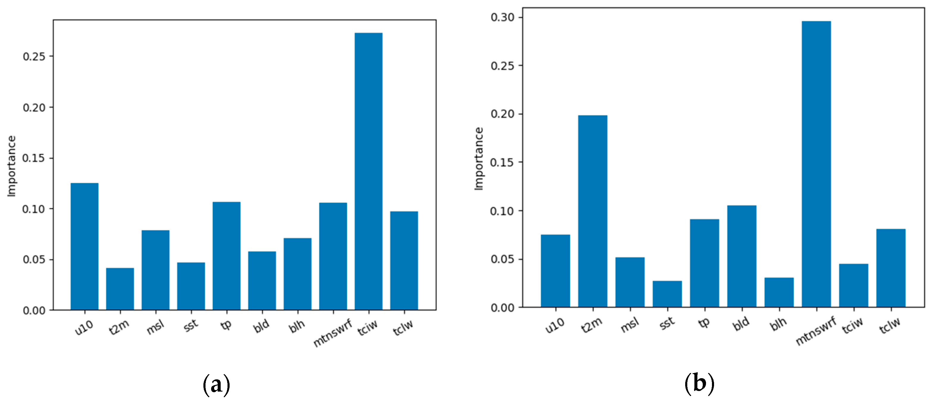
2.6. Random Forest Regression for Meteorological Factor Section

Weather affects aerosols in complicated ways and through various meteorological factors, such as temperature, wind, pressure, precipitation, solar radiation, cloud, etc. Since there are many potential meteorological factors that can affect aerosols, it is vital to find the influential factors before further analysis. In addition, the complicated relations and multi-dimension weather parameters made it hard for classical methods, such as polynomial regression, Bayesian linear regression or other methods [39], to explain the data. Based on these considerations, this work employs random forest regression method to measure the importance of different meteorological factors.

Random forest regression (RFR) [40] is a supervised learning algorithm based on ensemble learning. Random forest applies a number of decision trees on sub-samples and takes the average of regression results from each decision tree to improve accuracy and generalization. All sub-tree structures and node splitting parameters are optimized by minimizing the difference between regression results and actual data. The splitting condition of decision trees can reflect the importance of data features. Because the importance feature is more likely to divide the data into low-variance or low-entropy subset, the contribution on decreasing data impurity can be used as indicator for feature importance.

In this study, AOD data are considered as dependent variable while meteorological factors are considered as independent variables. In particular works, many libraries such as Pytorch and Tensorflow can be used to carry out machine learning algorithms. In this work, function RandomForestRegressor in sklearn is used for analyzing the importance of different meteorological factors. As for the parameters of RandomForestRegressor function, the number of trees is 100 and the maximum depth of the tree is 5. In addition, mean absolute error (MAE) is used as the criterion to measure the quality of a split at each node.

3. Results

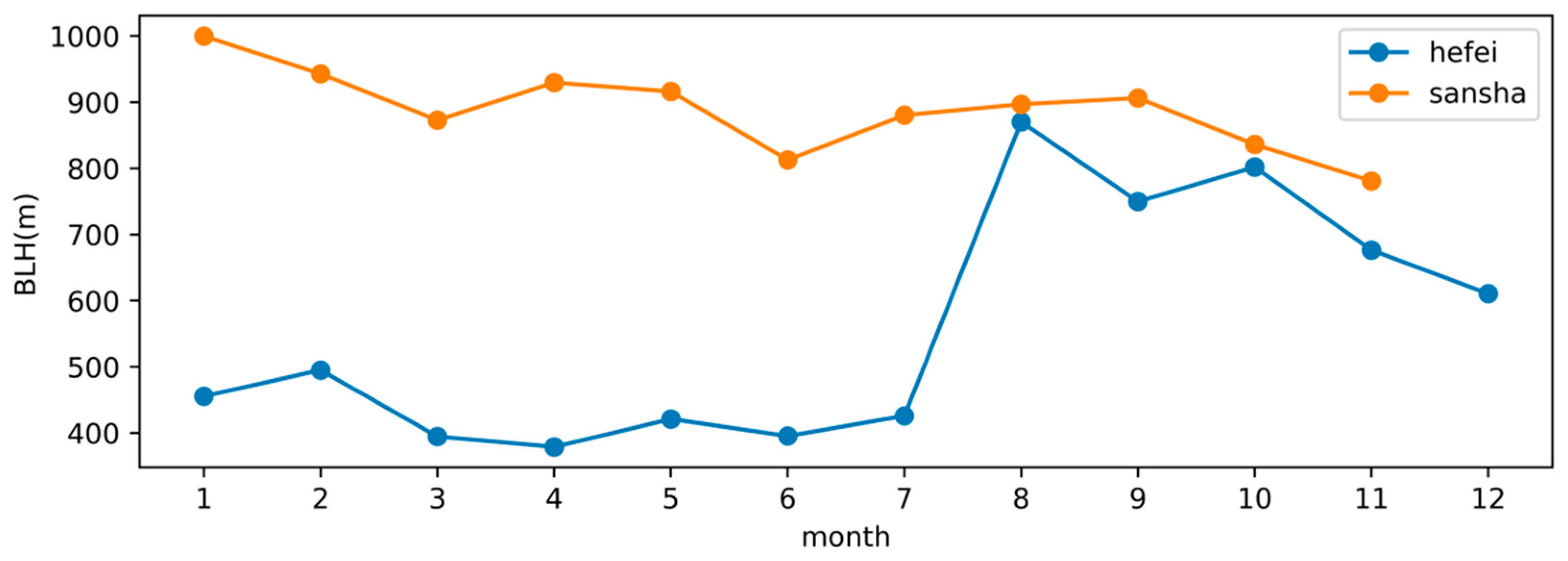
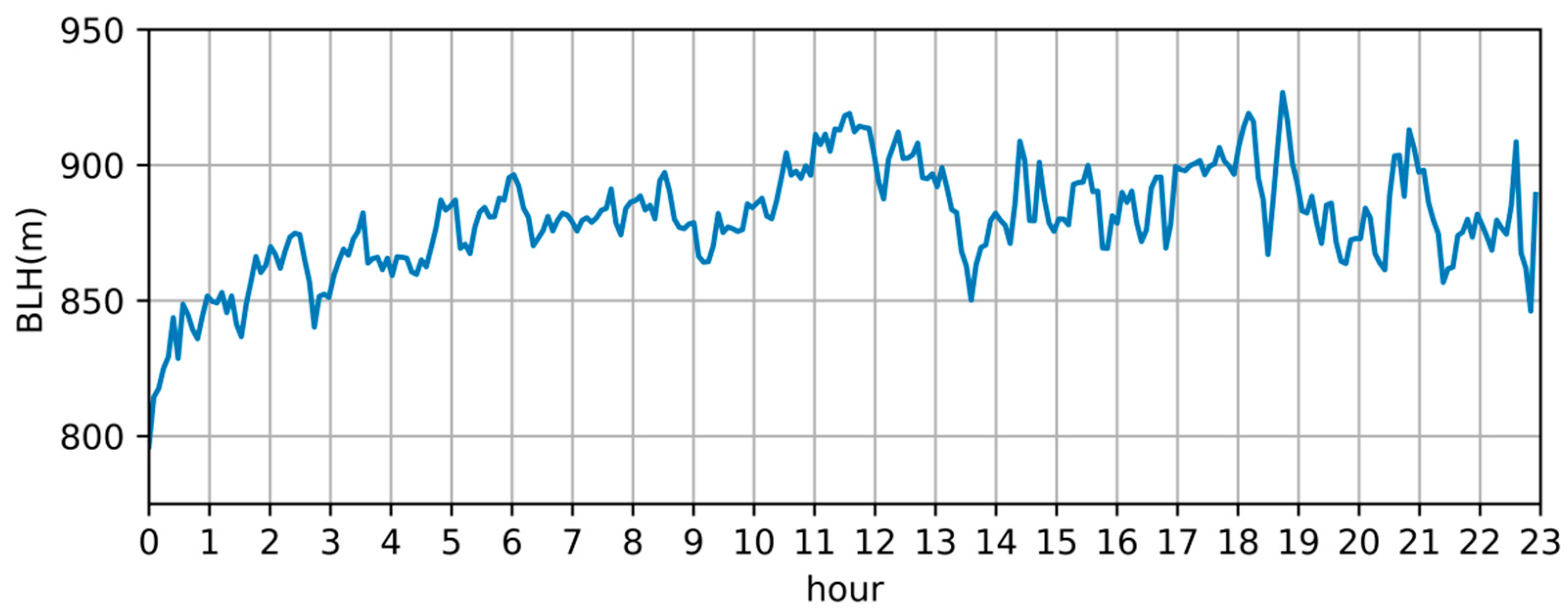
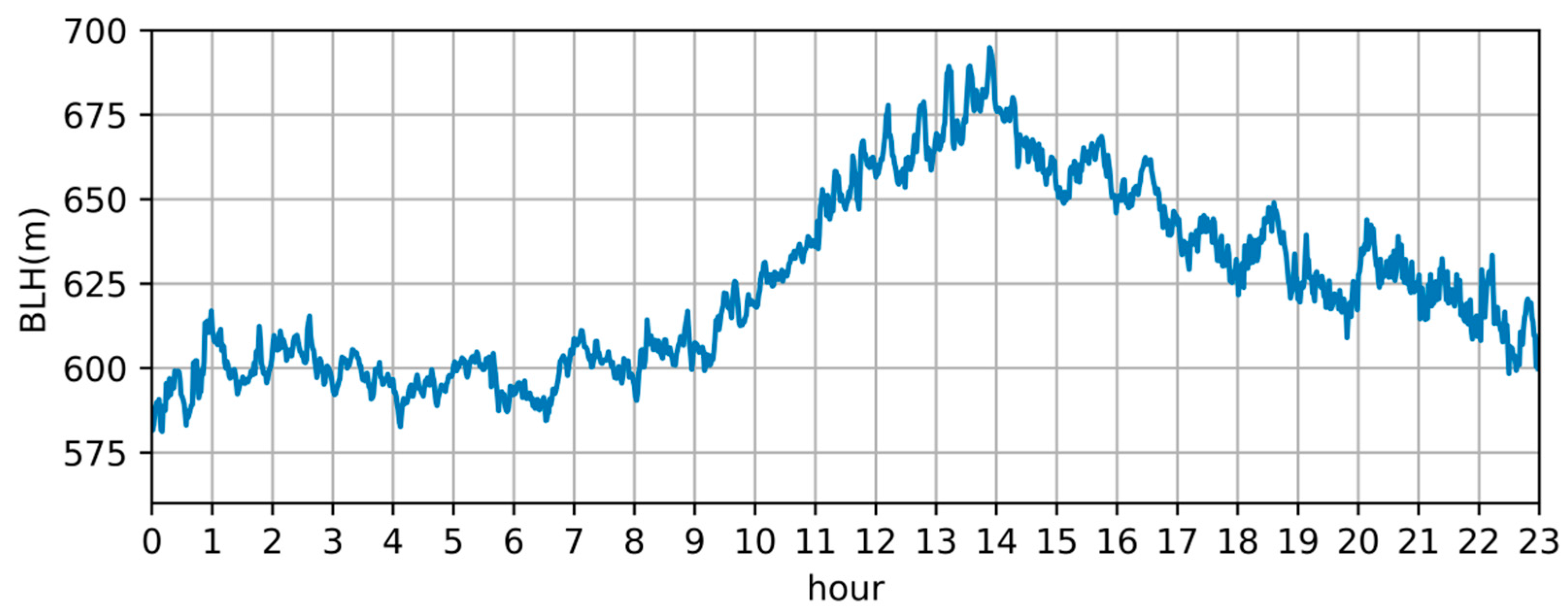
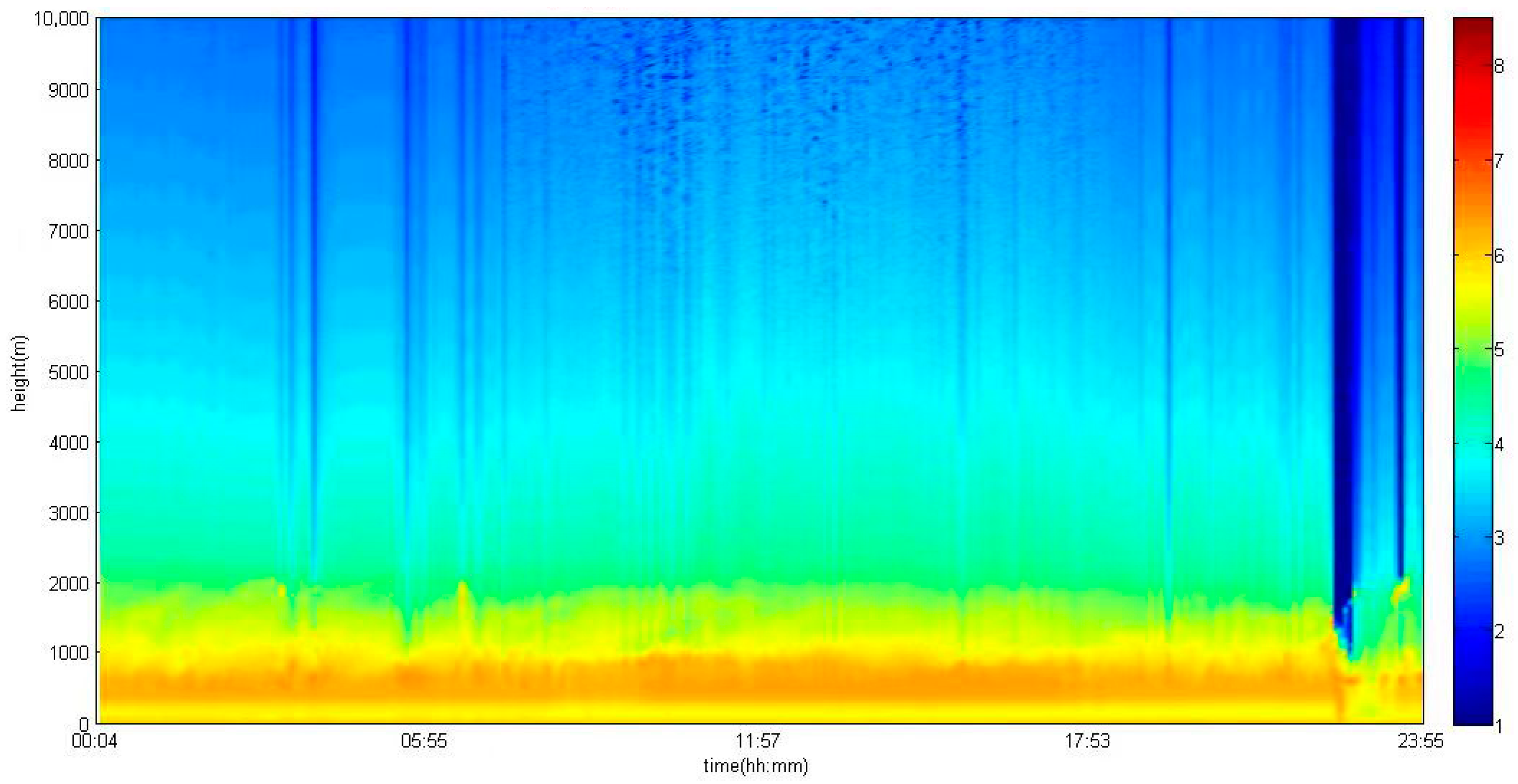
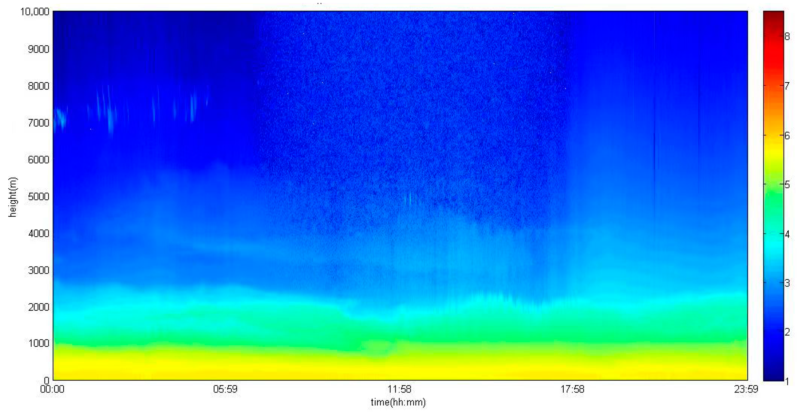
3.1. Planetary Boundary Layer Height

The boundary layer height can be calculated using the ideal fitting method described in Section 2.5 for each season. The four seasons are divided as: spring (March, April and May), summer (June, July and August), fall (September, October and November) and winter (December, January and February). The result depicts the average daily boundary layer height. As for Sansha in 2021, the average boundary layer height in spring, summer and winter is 906 m, 895 m and 902 m, showing a slight difference. On the contrary, in fall, average boundary layer height is the lowest (803 m). As for Hefei, the boundary layer height has the following relation: fall (752 m) > summer (617 m) > winter (513 m) > spring (395 m). In fall, the boundary layer height is the highest, with an average value 752 m. No matter whether Sansha or Hefei, BLH seasonal change is mainly associated with the rise and expansion of hot air. When the average temperature is high, the atmosphere will be expanded and lifted, which results in an increase in boundary layer height. It is also obvious that the BLH seasonal variation in Hefei is larger than Sansha. This is because temperature change is more apparent in Hefei than in Sansha.

The monthly average of BLH for both Sansha and Hefei is shown in Figure 1. Sansha’s average boundary layer height is higher than Hefei’s in every month. This is mainly because the average temperature in Sansha is higher than in Hefei. In addition, there is an obvious increase for Hefei’s BLH while Sansha’s BLH varies more smoothly, since the weather (especially temperature) changes significantly more in Hefei than in Sansha during a year. The standard deviation for monthly BLH of Sansha and Hefei is 59.2 and 170.0, respectively.

In addition, daily average data for the boundary layer height are also calculated. Sansha’s daily average variation in boundary layer height is shown in Figure 2, while Hefei’s daily average data are shown in Figure 3. As Figure 2 illustrates, the daily variation in boundary layer height in Sansha is not big. The standard deviation of Sansha’s daily BLH average is 19.6. According to the relation of BLH and temperature described before, the slow increase in BLH from 0 am to 11 am is due to a temperature increase in the morning. However, since the daily temperature variation is more significant in Hefei, the boundary layer height has a bigger variation, as shown in Figure 3. The increase in BLH from 0 am to 1 pm is due to the temperature increase in the morning. The decrease in BLH from 3 pm to 12 pm is due to the cool down in the evening. The standard deviation of Hefei’s daily BLH average is 26.69. Furthermore, the hourly average boundary layer height for Sansha and Hefei are 876.46 m and 623.92 m, respectively.

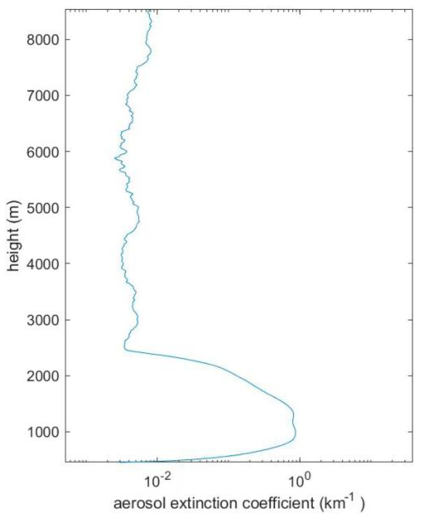
3.2. Aerosol Extinction Coefficient

After retrieving Mie lidar data using the Fernald method, we obtain daily extinction coefficient data for 2021. Figure 4 shows the aerosol extinction coefficient at different heights on 29 January 2021, 2:00 am. The aerosol extinction coefficient decreases after reaching a peak of 0.88 km^-1 at latitude 997.6 m. The coefficient decrease is due to the low aerosol density in the upper layer. However, the rapid decrease in aerosol extinction coefficient below 997.6 m is due to uncorrected overlap in the original data. From the surface to near 2509 m, the aerosol extinction coefficient has a variation of 0.88 km^-1. However, it remains almost constant above 2509 m, ranging from 0.0024 km^-1 to 0.0081 km^-1. This implies that aerosols are mainly distributed below 3 km, which is in concordance with previous studies [41].

The timely distribution of aerosol coefficient at different times and heights is shown in Figure 5 and Figure 6. In both Sansha and Hefei, with the increase in altitude, aerosol extinction coefficient decreases. The line between dark blue and bright blue in the pseudo-color map roughly represents a rapid aerosol concentration decrease in the upper air. The line is especially obvious in Figure 6. The dark blue stands for lower aerosol concentration while light blue represents higher aerosol concentration. In winter, this concentration decrease line in Hefei is around 2 km, while the line in Sansha is slightly above 4 km. This is due to the temperature difference. The latitude of Sansha (16°50′ N) is lower that Hefei (31°51′ N), so the temperature in Sansha is higher during winter. Furthermore, the rise in atmosphere temperature will result in atmosphere expansion and a rise in the concentration decrease line.

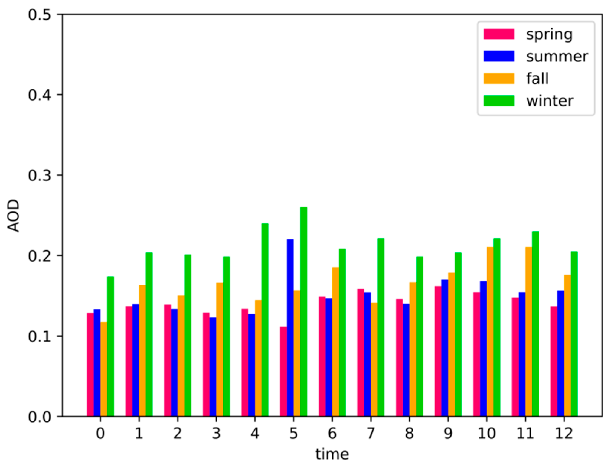
3.3. Aerosol Optical Depth

Aerosol optical depth can be calculated by integrating the extinction coefficient. As demonstrated in Figure 7, AOD in different seasons changes slightly from 0 am to 12 am. The daily average AOD for Sansha and Hefei is 0.2 and 0.4, respectively. For Sansha, average AOD for each season is as follows: 0.14 in spring, 0.18 in summer, 0.13 in fall and 0.21 in winter. Hefei’s seasonal average AOD is: 0.4 in spring, 0.31 in summer, 0.33 in fall and 0.48 in winter. Since Hefei is an economically developed city with high population while Sansha is on an island in the South China Sea, Hefei’s level of pollution is higher than Sansha’s. Furthermore, dense population and rapid urbanization can result in higher aerosol pollution [42] and higher AOD value [43].

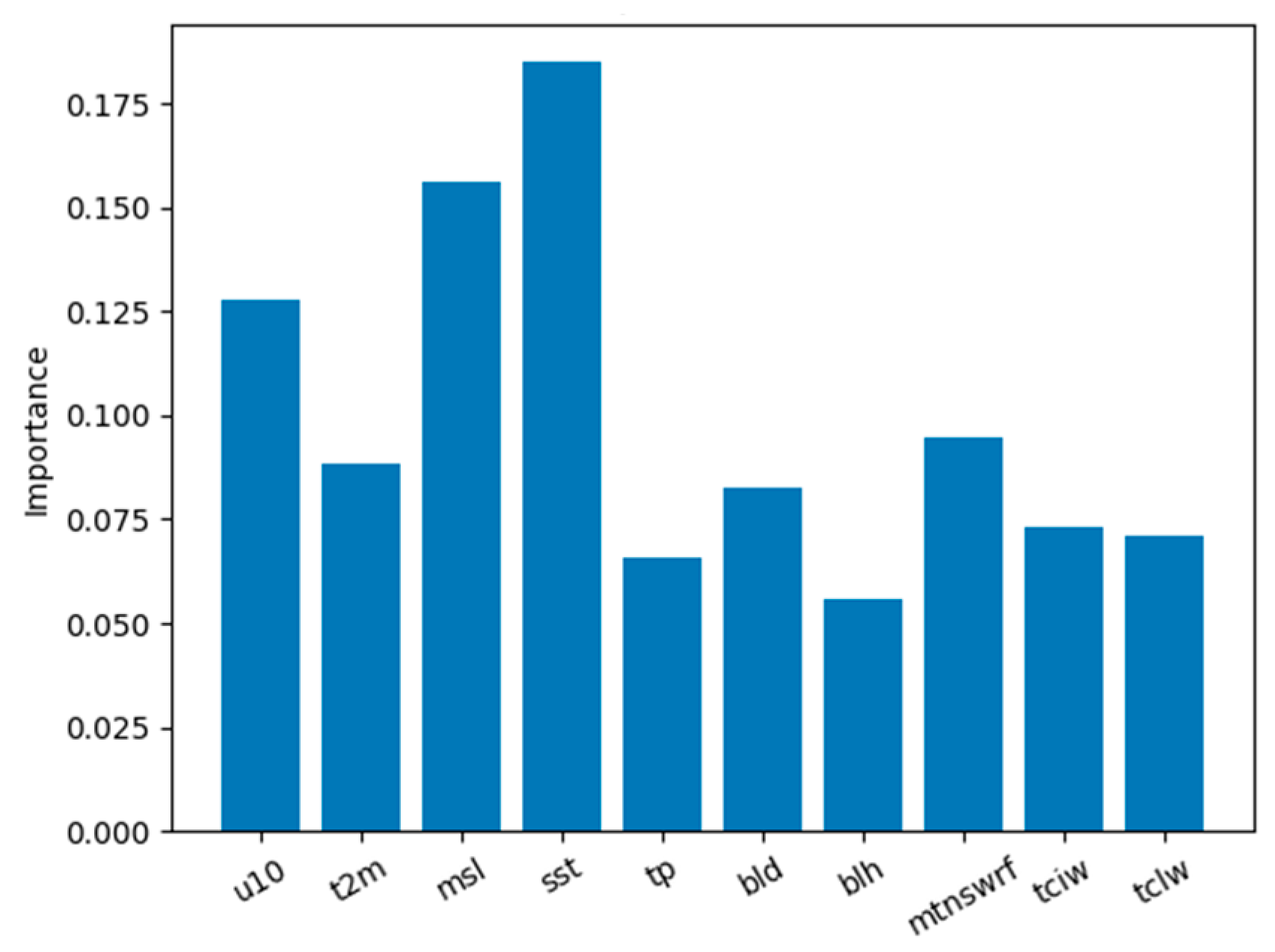
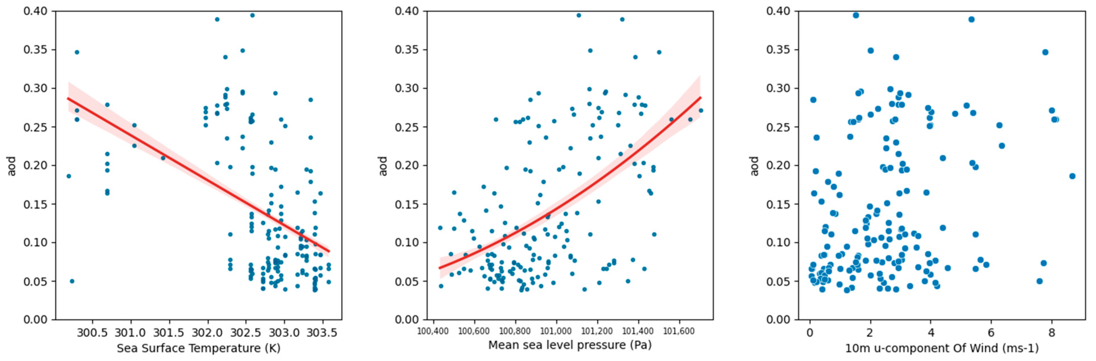
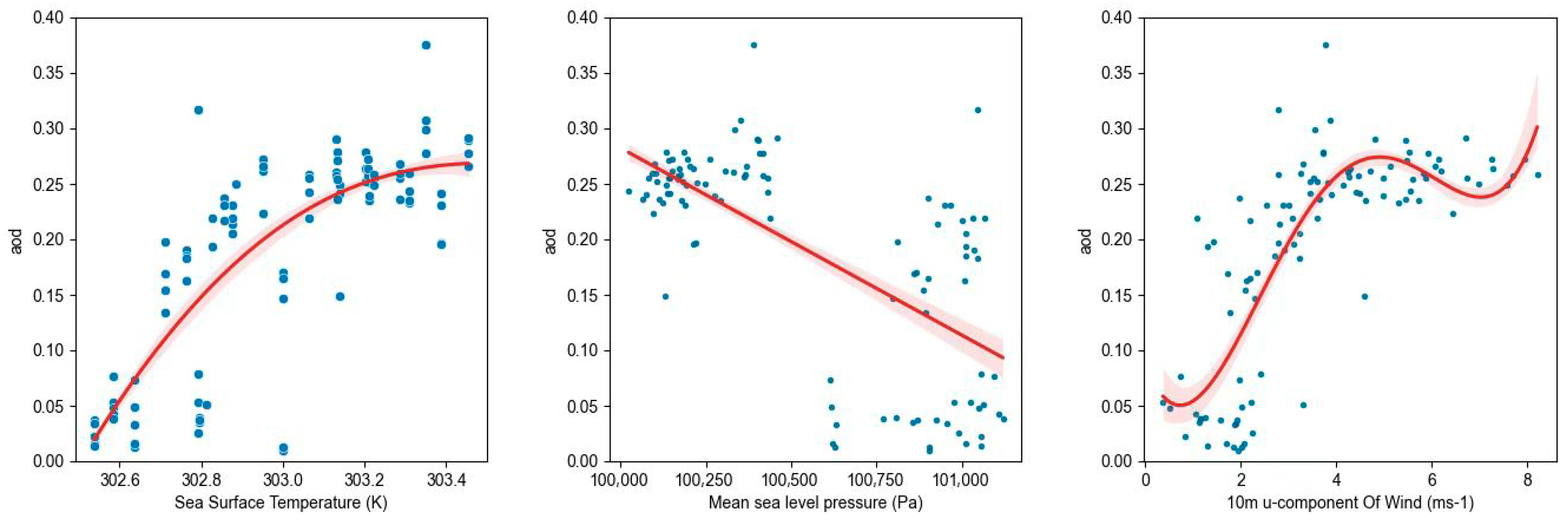
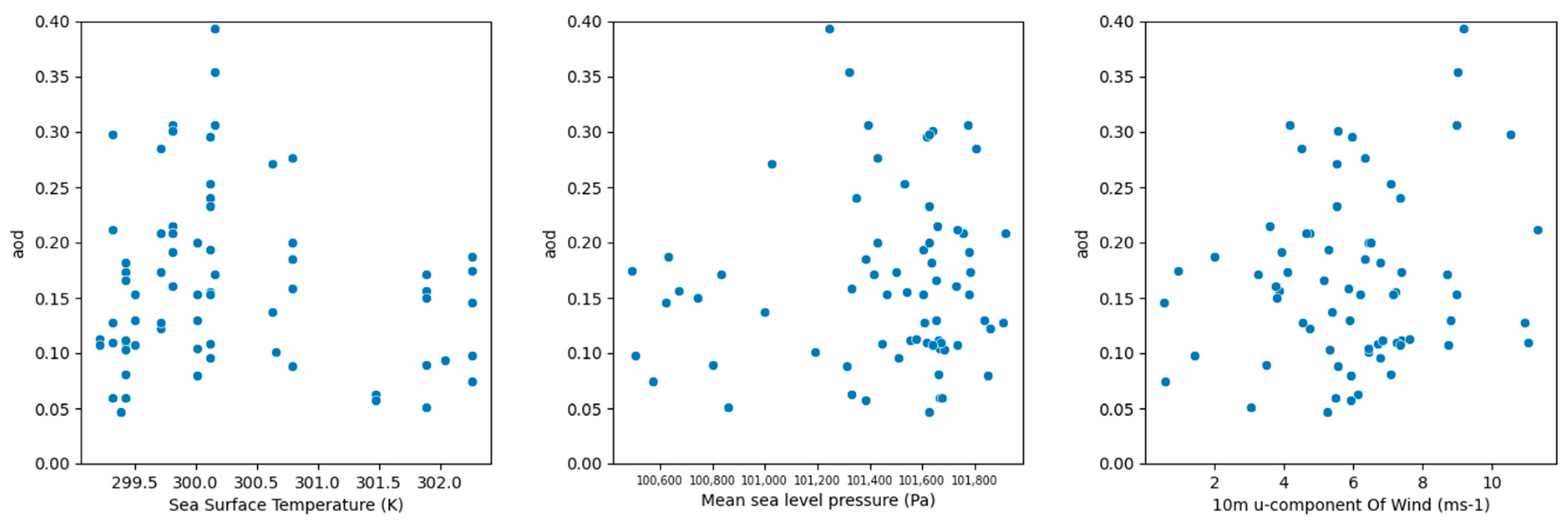
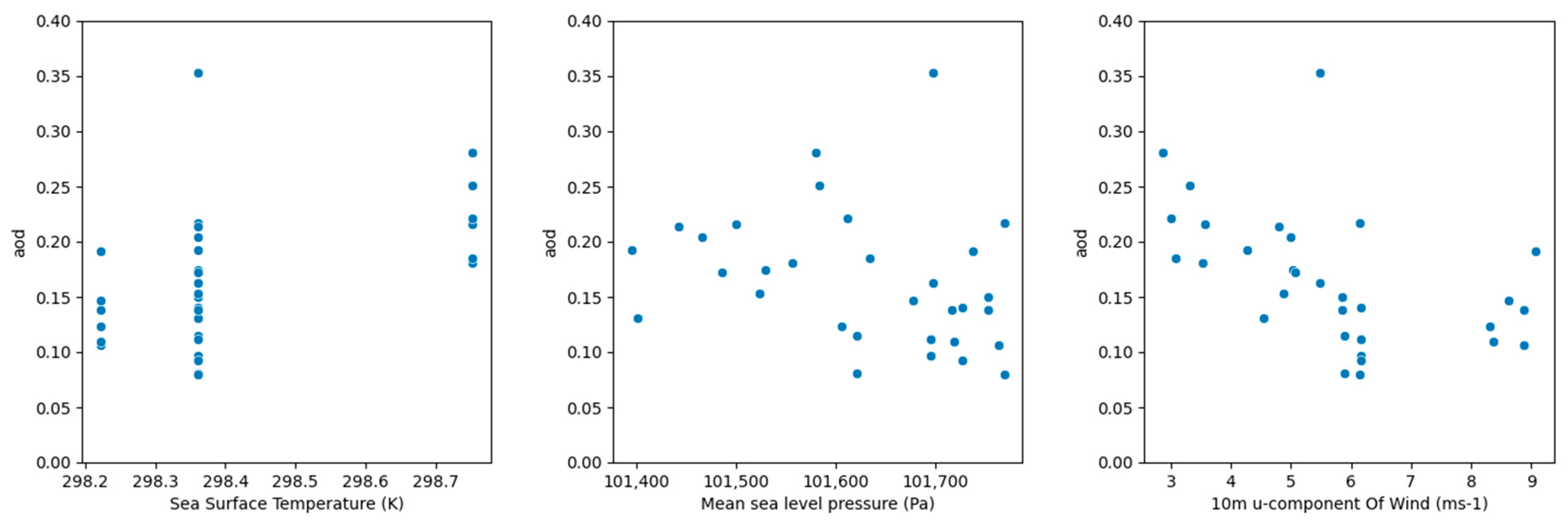
3.4. Aerosol Optical Depth and Meteorological Factors

To select influential meteorological factors, we use random forest regression to calculate each factor’s importance. Each factor’s importance reflects the data impurity decrease when dividing data with this factor. Figure 8 demonstrates each meteorological factor’s importance. Among all candidate meteorological factors, sea surface temperature (sst), mean sea level pressure (msl) and 10 m u-component of wind (u10) are the top three important factors that influence AOD, as shown in Figure 8. Some studies also verified the strong relation between AOD and sea surface temperature [44,45], mean sea level pressure [46] and 10 m u-component of wind [30].

To further understand how sst, msl and u10 may impact nighttime AOD in Sansha, we analyze AOD-meteorological factor relations in four seasons. Since only nighttime AOD data are selected, it is reasonable for radiation flux (mtnswrf) to have low data importance.

In spring (March, April and May), AOD has a negative correlation with sea surface temperature and a positive correlation with mean sea level pressure, as Figure 9 illustrated. However, there is no apparent relation between 10 m u-component of wind and AOD.

In summer (June, July and August), AOD is positively associated with sea surface temperature, as shown in the first sub-figure in Figure 10. When sea surface temperature is above 302.8 K, AOD is above 0.2. In addition, AOD and mean level pressure also have a weak negative correlation. When mean sea level pressure is below 100,500 Pa, AOD values gather around 0.25. When mean sea level pressure is above 100,500 Pa, AOD concentrates around 0.16 or 0.03. The third sub-figure in Figure 10 implies that AOD has a strong positive correlation with wind speed. When the 10 m u-component of wind is below 4 (ms⁻¹), AOD increases at a rate of 0.06. After wind speed reaches 4 (ms^-1), AOD remains constant around 0.25.

There are many ways that AOD and temperature can influence each other. One way for temperature to affect AOD is through the process of releasing salt particles. Waves and sea bubbles may release sea salt particles, which turn into marine aerosols [47]. The higher the temperature, the easier for the bubbles to break and release marine aerosols. Therefore, as temperature rises, aerosol concentration and AOD also increase, which is consistent with the result in Figure 10. However, in spring, aerosols may reduce solar radiation by aerosol–cloud interaction. In particular, an increase in cloud and cloud liquid water leads to a decrease in solar radiation absorption [48]. Thus, the increase in aerosol restrains temperature rise, as shown in Figure 9.

Many previous studies show that there is correlation between AOD and wind speed [30,49]. Furthermore, AOD in many near-continent marine areas has positive correlation with wind speed [50], as shown in Figure 10. This phenomenon can be explained by the following two reasons: Firstly, dust and aerosols on land can be transported to the ocean and become a part of marine aerosols. Secondly, the increase in wind speed itself can contribute to AOD, which is related with the breaking of waves and appearance of bubbles [51]. Stronger wind can break the wave and produce more bubbles on the water surface. Sea salt transforms into marine aerosol particles after the bubble in the sea surface is broken. Thus, the concentration of marine aerosols and AOD increases [52].

As for fall (September, October and November) and winter (December, January and February), AOD has no significant correlation with any selected meteorological factors (sst, msl and u10), referring to Figure 11 and Figure 12. To further verify this phenomenon, feature importance for only fall or winter is calculated using the same method described in Section 2.6. As illustrated in Figure 13, sst, msl and u10 do not have the highest feature importance, which means that they are not dominating factors in fall and winter.

Although many previous studies have revealed certain meteorological factor’s impact on aerosol, they cannot apply directly to the real marine environment. In some seasons, wind speed may have a dominating effect, while other factors have a weaker impact. However, in other seasons, temperature and other factors may play a key role. Thus, due to the temporal change and interaction between meteorological factors, the influential factor varies seasonally. Furthermore, relation between certain factors and aerosol may also change seasonally because other meteorological processes may affect their relation differently [53].

4. Conclusions

In this study, based on Mie lidar, we analyze the temporal variation in aerosols and the relation between AOD and meteorological factors in Sansha. Firstly, boundary layer height is calculated by an ideal fitting method. For Sansha, BLH ranges from 803 m to 906 m. Sansha’s BLH does not have obvious seasonal variation: spring (906 m), summer (895 m), fall (803 m) and winter (902 m). On the contrary, in Hefei, the boundary layer is highest in fall (752 m) and lowest in spring (395 m). We further explain this phenomenon using temperature variation. Secondly, using the Fernald algorithm, we inverse Mie lidar data and obtain the aerosol extinction coefficient. The aerosol extinction coefficient in Sansha varies from 0.0024 km^-1 to 0.88 km^-1. With the increase in altitude, the aerosol extinction coefficient decreases. Compared with the aerosol extinction coefficient distribution in Hefei, the upper layer of aerosol distribution in Sansha is higher. Then, average annual AOD in Sansha is 0.2, while average AOD in each season is: spring (0.14), summer (0.18), fall (0.13) and winter (0.21). Finally, after applying random forest regression, we select sea surface temperature, mean sea level pressure and 10 m u-component of wind as meteorological factors used for analysis. In summer and spring, there is apparent correlation between AOD and meteorological factors. However, in fall and winter, these factors do not impact AOD strongly.

References

1. Groß, S.; Tesche, M.; Freudenthaler, V.; Toledano, C.; Wiegner, M.; Ansmann, A.; Althausen, D.; Seefeldner, M. Characterization of Saharan dust, marine aerosols and mixtures of biomass-burning aerosols and dust by means of multi-wavelength depolarization and Raman lidar measurements during SAMUM 2. Tellus B Chem. Phys. Meteorol. 2011, 63, 706–724. [Google Scholar] [CrossRef]
2. Rosenfeld, D.; Dai, J.; Yu, X.; Yao, Z.; Xu, X.; Yang, X.; Du, C. Inverse relations between amounts of air pollution and orographic precipitation. Science 2007, 315, 1396–1398. [Google Scholar] [CrossRef] [PubMed]
3. O’Dowd, C.D.; De Leeuw, G. Marine aerosol production: A review of the current knowledge. Philos. Trans. R. Soc. A Math. Phys. Eng. Sci. 2007, 365, 1753–1774. [Google Scholar] [CrossRef]
4. Twomey, S. Pollution and the planetary albedo. Atmos. Environ. 1974, 8, 1251–1256. [Google Scholar] [CrossRef]
5. Väkevä, M.; Hämeri, K.; Puhakka, T.; Nilsson, E.D.; Hohti, H.; Mäkelä, J.M. Effects of meteorological processes on aerosol particle size distribution in an urban background area. J. Geophys. Res. Atmos. 2000, 105, 9807–9821. [Google Scholar] [CrossRef]
6. Hussein, T.; Karppinen, A.; Kukkonen, J.; Härkönen, J. Meteorological dependence of size-fractionated number concentrations of urban aerosol particles. Atmos. Environ. 2006, 40, 1427–1440. [Google Scholar] [CrossRef]
7. Che, H.; Gui, K.; Xia, X.; Wang, Y.; Holben, B.N.; Goloub, P.; Cuevas-Agulló, E.; Wang, H.; Zheng, Y.; Zhao, H.; et al. Large contribution of meteorological factors to inter-decadal changes in regional aerosol optical depth. Atmos. Chem. Phys. 2019, 19, 10497–10523. [Google Scholar] [CrossRef]
8. Liu, X.; Penner, J.E.; Das, B.; Bergmann, D.; Rodriguez, J.M.; Strahan, S.; Wang, M.; Feng, Y. Uncertainties in global aerosol simulations: Assessment using three meteorological data sets. J. Geophys. Res. Atmos. 2007, 112, D11212. [Google Scholar] [CrossRef]
9. Zaman, N.A.F.K.; Kanniah, K.D.; Kaskaoutis, D.G. Estimating particulate matter using satellite based aerosol optical depth and meteorological variables in Malaysia. Atmos. Res. 2017, 193, 142–162. [Google Scholar] [CrossRef]
10. Sathe, Y.; Kulkarni, S.; Gupta, P.; Kaginalkar, A.; Islam, S.; Gargava, P. Application of Moderate Resolution Imaging Spectroradiometer (MODIS) Aerosol Optical Depth (AOD) and Weather Research Forecasting (WRF) model meteorological data for assessment of fine particulate matter (PM2.5) over India. Atmos. Pollut. Res. 2019, 10, 418–434. [Google Scholar] [CrossRef]
11. So, C.K.; Cheng, C.M.; Tsui, K.C. Weather and environmental monitoring using MODIS AOD data in Hong Kong, China. In Proceedings of the First International Symposium on Cloud-prone & Rainy Areas Remote Sensing, Hong Kong, China, 6–8 October 2005. [Google Scholar]
12. Letcher, T.; Cotton, W.R. The effect of pollution aerosol on wintertime orographic precipitation in the Colorado Rockies using a simplified emissions scheme to predict CCN concentrations. J. Appl. Meteorol. Climatol. 2014, 53, 859–872. [Google Scholar] [CrossRef]
13. Gao, M.; Sherman, P.; Song, S.; Yu, Y.; Wu, Z.; Mcelroy, M.B. Seasonal prediction of Indian wintertime aerosol pollution using the ocean memory effect. Sci. Adv. 2019, 5, eaav4157. [Google Scholar] [CrossRef]
14. Acosta Navarro, J.C.; Varma, V.; Riipinen, I.; Selan, Ø.; Kirkevåg, A.; Struthers, H.; Iversen, T.; Hansson, H.-C.; Ekman, A.M.L. Amplification of Arctic warming by past air pollution reductions in Europe. Nat. Geosci. 2016, 9, 277–281. [Google Scholar] [CrossRef]
15. Westervelt, D.M.; Mascioli, N.R.; Fiore, A.M.; Conley, A.J.; Lamarque, J.-F.; Shindell, D.T.; Faluvegi, G.; Previdi, M.; Correa, G.; Horowitz, L.W. Local and remote mean and extreme temperature response to regional aerosol emissions reductions. Atmos. Chem. Phys. 2020, 20, 3009–3027. [Google Scholar] [CrossRef]
16. Mahowald, N.M.; Scanza, R.; Brahney, J.; Goodale, C.L.; Hess, G.P.; Moore, J.K.; Neff, J. Aerosol deposition impacts on land and ocean carbon cycles. Curr. Clim. Chang. Rep. 2017, 3, 16–31. [Google Scholar] [CrossRef]
17. Bauer, S.E.; Tsigaridis, K.; Miller, R. Significant atmospheric aerosol pollution caused by world food cultivation. Geophys. Res. Lett. 2016, 43, 5394–5400. [Google Scholar] [CrossRef]
18. Kaufman, Y.J.; Tanré, D.; Boucher, O. A satellite view of aerosols in the climate system. Nature 2002, 419, 215–223. [Google Scholar] [CrossRef]
19. Zhang, L.; Zheng, X.S. Spatial-temporal Variation of Aerosol Optical Properties in Coastal Region, China Based on CALIPSO Data. J. Earth Sci. Env. 2021, 43, 1033–1049. [Google Scholar]
20. Su, Y.; Han, Y.; Luo, H.; Zhang, Y.; Shao, S.; Xie, X. Physical-Optical Properties of Marine Aerosols over the South China Sea: Shipboard Measurements and MERRA-2 Reanalysis. Remote Sens. 2022, 14, 2453. [Google Scholar] [CrossRef]
21. Novakov, T.; Hegg, D.A.; Hobbs, P.V. Airborne measurements of carbonaceous aerosols on the East Coast of the United States. J. Geophys. Res. Atmos. 1997, 102, 30023–30030. [Google Scholar] [CrossRef]
22. Haarig, M.; Ansmann, A.; Gasteiger, J.; Kandler, K.; Althausen, D.; Baars, H.; Radenz, M.; Farrell, D.A. Dry versus wet marine particle optical properties: RH dependence of depolarization ratio, backscatter, and extinction from multiwavelength lidar measurements during SALTRACE. Atmos. Chem. Phys. 2017, 17, 14199–14217. [Google Scholar] [CrossRef] [Green Version]
23. Groß, S.; Esselborn, M.; Weinzierl, B.; Wirth, M.; Fix, A.; Petzold, A. Aerosol classification by airborne high spectral resolution lidar observations. Atmos. Chem. Phys. 2013, 13, 2487–2505. [Google Scholar] [CrossRef]
24. Sharma, S.K.; Lienert, B.R.; Porter, J.N. Scanning lidar measurements of marine aerosol fields at a coastal site in Hawaii. Lidar Remote Sens. Ind. Environ. Monit. SPIE 2001, 4153, 159–166. [Google Scholar]
25. Omar, A.H.; Winker, D.M.; Kittaka, C.; Vaughan, M.A.; Liu, Z.; Hu, Y.; Trepte, C.R.; Rogers, R.R.; Lee, K.-P.A.; Kuehn, R.E.; et al. The CALIPSO automated aerosol classification and lidar ratio selection algorithm. J. Atmos. Ocean. Technol. 2009, 26, 1994–2014. [Google Scholar] [CrossRef]
26. Ma, X.; Zhang, H.; Han, G.; Mao, F.; Xu, H.; Shi, T.; Hu, H.; Sun, T.; Gong, W. A Regional Spatiotemporal Downscaling Method for CO2 Columns. IEEE Trans. Geosci. Remote Sens. 2021, 59, 8084–8093. [Google Scholar] [CrossRef]
27. Vlemmix, T.; Piters, A.J.M.; Stammes, P.; Wang, P.; Levelt, P.F. Retrieval of tropospheric NO2 using the MAX-DOAS method combined with relative intensity measurements for aerosol correction. Atmos. Meas. Tech. 2010, 3, 1287–1305. [Google Scholar] [CrossRef]
28. Lin, P.; Hu, M.; Wu, Z.; Niu, Y.; Zhu, T. Marine aerosol size distributions in the springtime over China adjacent seas. Atmos. Environ. 2007, 41, 6784–6796. [Google Scholar] [CrossRef]
29. Fu, H.; Zheng, M.; Yan, C.; Li, X.; Gao, H.; Yao, X.; Guo, Z.; Zhang, Y. Sources and characteristics of fine particles over the Yellow Sea and Bohai Sea using online single particle aerosol mass spectrometer. J. Environ. Sci. 2015, 29, 62–70. [Google Scholar] [CrossRef]
30. Sun, Q.; Tang, D.L.; Levy, G.; Shi, P. Variability of aerosol optical thickness in the tropical Indian Ocean and South China Sea during spring intermonsoon season. Int. J. Remote Sens. 2018, 39, 4531–4549. [Google Scholar] [CrossRef]
31. Onasch, T.B.; Siefert, R.L.; Brooks, S.D.; Prenni, A.J.; Murray, B.; Wilson, M.A.; Tolbert, M.A. Infrared spectroscopic study of the deliquescence and efflorescence of ammonium sulfate aerosol as a function of temperature. J. Geophys. Res. Atmos. 1999, 104, 21317–21326. [Google Scholar] [CrossRef]
32. Liu, B.; Ma, X.; Ma, Y.; Li, H.; Jin, S.; Fan, R.; Gong, W. The relationship between atmospheric boundary layer and temperature inversion layer and their aerosol capture capabilities. Atmos. Res. 2022, 271, 106121. [Google Scholar] [CrossRef]
33. Shi, T.; Han, G.; Ma, X.; Gong, W.; Chen, W.; Liu, J.; Zhang, X.; Pei, Z.; Gou, H.; Bu, L. Quantifying CO2 uptakes over oceans using LIDAR: A tentative experiment in Bohai bay. Geophys. Res. Lett. 2021, 48, e2020GL091160. [Google Scholar] [CrossRef]
34. Stamnes, S.; Hostetler, C.; Ferrare, R.; Burton, S.; Liu, X.; Hair, J.; Hu, Y.; Wasilewski, A.; Martin, W.; van Diedenhoven, B.; et al. Simultaneous polarimeter retrievals of microphysical aerosol and ocean color parameters from the “MAPP” algorithm with comparison to high-spectral-resolution lidar aerosol and ocean products. Appl. Opt. 2018, 57, 2394–2413. [Google Scholar] [CrossRef]
35. Alarcon, M.C. A Mie Lidar System for Atmospheric Monitoring: Design Considerations. Trans. Nat. Acad. Sci. Technol. 1993, 15, 93–106. [Google Scholar]
36. Hersbach, H.; Bell, B.; Berrisford, P.; Biavati, G.; Horányi, A.; Muñoz-Sabater, J.; Nicolas, J.; Peubey, C.; Radu, R.; Schepers, D.; et al. ERA5 hourly data on single levels from 1979 to present. Copernic. Clim. Chang. Serv. (C3S) Clim. Data Store (CDS). Available online: https://doi.org/10.24381/cds.bd0915c6 (accessed on 1 May 2022). [CrossRef]
37. Fernald, F.G.; Herman, B.M.; Reagan, J.A. Determination of aerosol height distributions by lidar. J. Appl. Meteorol. Climatol. 1972, 11, 482–489. [Google Scholar] [CrossRef]
38. Steyn, D.G.; Baldi, M.; Hoff, R.M. The detection of mixed layer depth and entrainment zone thickness from lidar backscatter profiles. J. Atmos. Ocean. Technol. 1999, 16, 953–959. [Google Scholar] [CrossRef]
39. Dong, Y.; Shi, W.; Du, B.; Hu, X.; Zhang, L. Asymmetric weighted logistic metric learning for hyperspectral target detection. IEEE Trans. Cybern. 2021. [Google Scholar] [CrossRef]
40. Ho, T.K. Random decision forests. Proc. 3rd Int. Conf. Doc. Anal. Recognit. IEEE 1995, 1, 278–282. [Google Scholar]
41. Li, Y.; Wang, B.; Lee, S.Y.; Zhang, Z.; Wang, Y.; Dong, W. Micro-Pulse Lidar Cruising Measurements in Northern South China Sea. Remote Sens. 2020, 12, 1695. [Google Scholar] [CrossRef]
42. Tie, X.; Brasseur, G.P.; Zhao, C.S.; Granier, C.; Massie, S.; Qin, Y.; Wang, P.; Wang, G.; Yang, P.; Richter, A. Chemical characterization of air pollution in Eastern China and the Eastern United States. Atmos. Environ. 2006, 40, 2607–2625. [Google Scholar] [CrossRef]
43. He, Q.; Zhang, M.; Huang, B. Spatio-temporal variation and impact factors analysis of satellite-based aerosol optical depth over China from 2002 to 2015. Atmos. Environ. 2016, 129, 79–90. [Google Scholar] [CrossRef]
44. Zhang, W.; He, Q.; Wang, H.; Cao, K.; He, S. Factor analysis for aerosol optical depth and its prediction from the perspective of land-use change. Ecol. Indic. 2018, 93, 458–469. [Google Scholar] [CrossRef]
45. Zábori, J.; Matisāns, M.; Krejci, R.; Nilsson, E.D.; Ström, J. Artificial primary marine aerosol production: A laboratory study with varying water temperature, salinity, and Succinic acid concentration. Atmos. Chem. Phys. 2012, 12, 10709–10724. [Google Scholar] [CrossRef] [Green Version]
46. Gillett, N.P.; Fyfe, J.C.; Parker, D.E. Attribution of observed sea level pressure trends to greenhouse gas, aerosol, and ozone changes. Geophys. Res. Lett. 2013, 40, 2302–2306. [Google Scholar] [CrossRef]
47. Kiliyanpilakkil, V.P.; Meskhidze, N. Deriving the effect of wind speed on clean marine aerosol optical properties using the A-Train satellites. Atmos. Chem. Phys. 2011, 11, 11401–11413. [Google Scholar] [CrossRef]
48. Huang, Y.; Dickinson, R.E.; Chameides, W.L. Impact of aerosol indirect effect on surface temperature over East Asia. Proc. Natl. Acad. Sci. USA 2006, 103, 4371–4376. [Google Scholar] [CrossRef]
49. Levy, G.; Vignudelli, S.; Gower, J. Enabling earth observations in support of global, coastal, ocean, and climate change research and monitoring. Int. J. Remote Sens. 2018, 39, 4287–4292. [Google Scholar] [CrossRef]
50. Mishchenko, M.I.; Geogdzhayev, I.V. Satellite remote sensing reveals regional tropospheric aerosol trends. Opt. Express 2007, 15, 7423–7438. [Google Scholar] [CrossRef]
51. Huang, H.; Thomas, G.E.; Grainger, R.G. Relationship between wind speed and aerosol optical depth over remote ocean. Atmos. Chem. Phys. 2010, 10, 5943–5950. [Google Scholar] [CrossRef]
52. Lewis, E.R.; Schwartz, S.E. Measurements and models of quantities required to evaluate sea salt aerosol production fluxes. Sea Salt Aerosol Prod. Mech. Methods Meas. Models 2004, 152, 119–297. [Google Scholar]
53. Knippertz, P.; Todd, M.C. Mineral dust aerosols over the Sahara: Meteorological controls on emission and transport and implications for modeling. Rev. Geophys. 2012, 50. [Google Scholar] [CrossRef]
Figure 1. Monthly average of boundary layer height in Sansha and Hefei. The absence of data in December in Sansha is due to the lack of lidar data.
Atmosphere 13 01511 g001
Figure 2. Daily average of boundary layer height in Sansha.
Atmosphere 13 01511 g002
Figure 3. Daily average of boundary layer height in Hefei.
Atmosphere 13 01511 g003
Figure 4. Aerosol extinction coefficient on 29 January 2021, 2:00 am, local time.
Atmosphere 13 01511 g004
Figure 5. Pseudo-color map for aerosol extinction coefficient ( 10 4   m 1 ) in Sansha on 11 February 2021.
Atmosphere 13 01511 g005
Figure 6. Pseudo color map for aerosol extinction coefficient ( 10 4   m 1 ) in Hefei on 11 February 2021.
Atmosphere 13 01511 g006
Figure 7. Seasonal average AOD in Sansha.
Atmosphere 13 01511 g007
Figure 8. Feature importance of candidate meteorological factors.
Atmosphere 13 01511 g008
Figure 9. AOD-meteorological relation in spring.
Atmosphere 13 01511 g009
Figure 10. AOD-meteorological relation in summer.
Atmosphere 13 01511 g010
Figure 11. AOD-meteorological relation in fall.
Atmosphere 13 01511 g011
Figure 12. AOD-meteorological relation in winter.
Atmosphere 13 01511 g012
Figure 13. Feature importance of candidate meteorological factors (a) fall; (b) winter.
Atmosphere 13 01511 g013