A Quantizing Method for Atmospheric Environment Impact Post-Assessment of Highways Based on Computational Fluid Dynamics Model

Abstract

The post-assessment of highway atmospheric environmental impacts was limited by the traditional air pollution prediction model, which cannot adapt to complex terrain and complex obstacle scenes. The traditional model has a single evaluation index, which cannot accurately evaluate and predict the transient and long-term emissions of various pollutants. Based on the computational fluid dynamics model, this work establishes a post-assessment method of the atmospheric environment impact of the Beijing–Chengde Expressway construction project. The main pollution factors NOx and CO of highway traffic for transmission and diffusion simulation analysis were selected. The influence law of traffic function, environmental impact, meteorological conditions, and landform on the diffusion of pollution factors in complex tunnel sections were analyzed. It concludes that the pollution within 200 m along the expressway is severe and mainly concentrated in the tunnel entrance and gully area. The NOx concentration is generally higher than CO. The environmental quality is not up to standard and has a diffusion trend with increased traffic flow, operation time, wind speed, wind temperature, and wind direction frequency. The research results can provide theoretical guidance and technical support for the scientific post-assessment of highway environmental impact under complex conditions.

1. Introduction

Since the 1980s, highway construction in China has developed rapidly. By the end of 2021, China had 16 million kilometers of highways, including 528.07 million kilometers of highways nationwide [1]. The rapid development of highways has promoted the growth of the national and regional economies along the line. At the same time, the number of cars has exploded; the number of motor vehicles in China reached 310 million in 2017, with an average annual growth rate of about 5.9%, causing a series of environmental problems [2]. According to the annual report on Environmental Management of Motor Source of China, in 2020, the CO and NOx emissions from vehicles exceeded 90% of the total pollutant emissions, and the exhaust pollution continued to increase with the growth of highway operation time and the increase of traffic volume [3]. In addition, experimental data show that vehicle exhaust pollutants seriously impact human health and are prone to increase the risk of lung cancer, respiratory tract, and cardiovascular diseases [4,5,6,7,8]. Therefore, the post-assessment of the atmospheric environmental impact after the highway construction project comes into service for 3–5 years is of great significance. It is especially true for the comprehensive assessment of the actual impact of vehicle emissions on the atmospheric environment along the line, the inspection and verification of the implementation status and operation effect of pollution prevention and control measures along the highway, and the proposal of improvement measures for air pollution prevention and control [9].

The difficulty of post-assessment of highway atmospheric environment impact is that the transmission and diffusion of pollutants in the atmosphere is complicated and controlled by many factors. Airflow can diffuse and dilute atmospheric pollutants to harmless concentrations in barrier-free environments. However, in natural settings, many factors affect them, particularly meteorological factors (wind, turbulence, temperature inversion, and atmospheric stability), which play a decisive role. At the same time, underlying surface conditions such as terrain, buildings, and trees also play an essential role in the aggregation or disappearance of pollutants [10]. The semi-enclosed environment formed by the tunnel significantly impacts the pollutant diffusion in the highway vehicle exhaust pollution diffusion. Compared with the open road section, the pollutant concentration at the tunnel entrance increases significantly [11]. According to the city air quality report for the Barbican, London, UK [12], air pollution in the tunnel is quite severe, with the concentration of pollutants such as carbon monoxide (CO) and nitrogen dioxide (NO₂) dramatically exceeding the EU mean annual target. The average monthly NO₂ concentration in the Beech Street Tunnel in the City of London was 30% higher than the EU target. Similar results of severe air pollution in road tunnels are also revealed by Keyte et al. [13], Kim et al. [14], and Wingfors et al. [15].

Given the above problems, many models of atmospheric pollution diffusion have formed worldwide. Among them, the WRF-Chem model, developed by the American Meteorological Society and American Environmental Protection Agency, is a newly developed coupling model of regional atmospheric dynamics and atmospheric chemistry in the US. It has stronger vitality and for that reason, the meteorological model, which is closely concerned chemical transportation model, achieves true online transmission coupling in time and space [16]. Taseko et al. established the urban street model (USM) to analyze the diffusion and simulation of air pollutants [17]. Tim et al. used UKIAM to examine the effects of SO₂, NOx, NH₃, PM₁₀, and PM_2.5 on air pollution [18]; Elsa Aristodemou et al. used FLUIDITY to study the effects of tall buildings on nearby airflow and pollutant diffusion. Combined with the LES (large eddy simulation) method, the prediction results were significantly improved [19]. However, it is still impossible to accurately and comprehensively simulate the atmospheric flow and the diffusion of pollutants in complex environments and quantify the impact of obstacles such as complex terrain, buildings, surface vegetation, and various meteorological conditions on atmospheric diffusion, mechanical and thermal turbulence, and the transient and long-term emission of various pollutants.

Currently, the numerical simulation of atmospheric environment prediction in China’s relatively mature pollutant concentration prediction models includes the Gaussian diffusion model, Ministry of Transportation atmospheric pollutant concentration prediction model, and linear regression prediction model. The empirical method based on the Gaussian diffusion model is often used in international prediction, so the Gaussian model is also recommended in the atmospheric guidelines for environmental impact assessment in China. However, the traditional prediction model of air pollution based on the Gaussian model is difficult to adapt to the simulation analysis of pollution factors under complex terrain conditions. Therefore, the atmospheric environment analysis, assessment, and prediction cannot effectively provide technical support for environmental treatment.

This paper aims to apply CFD, widely used in the micro-scale diffusion simulation of urban environmental pollutants [20,21,22], to the diffusion simulation transmission and concentration prediction of highway air pollutants. In addition, considering many factors that affect the transmission and diffusion of pollutants in the road area, the diffusion law is analyzed to effectively predict the environmental impact of highway air pollutants under complex environmental conditions. Specifically, compared with the traditional Gaussian model, the CFD model considers many factors affecting the transport and diffusion of pollutants in the road area, such as wind, end-stream, temperature, humidity, air pressure, underlying surface, and human activities. It can also effectively predict the effect of obstacles on the wind direction and pollutants diffusion in complex environmental conditions [23]. In fact, it has been successfully applied to simulate pollutant dispersion in real urban environments [24,25,26,27,28,29,30,31]. We show that the simulated transmission of vehicle exhaust pollution diffusion under complex road conditions is closely related to traffic function, environmental impact, meteorological conditions, landform, and other factors. In addition, the main pollution factor of automobile exhaust is identified as NOx, and it is accurately predicted that the pollutants will significantly impact the environment in the future.

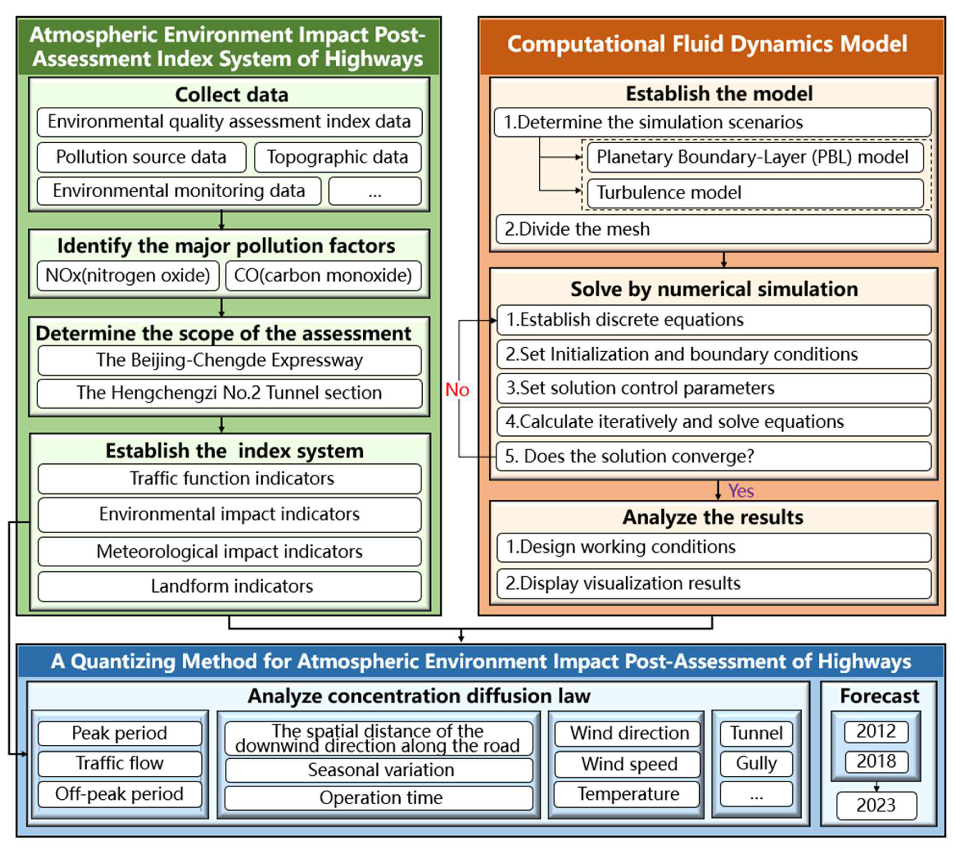
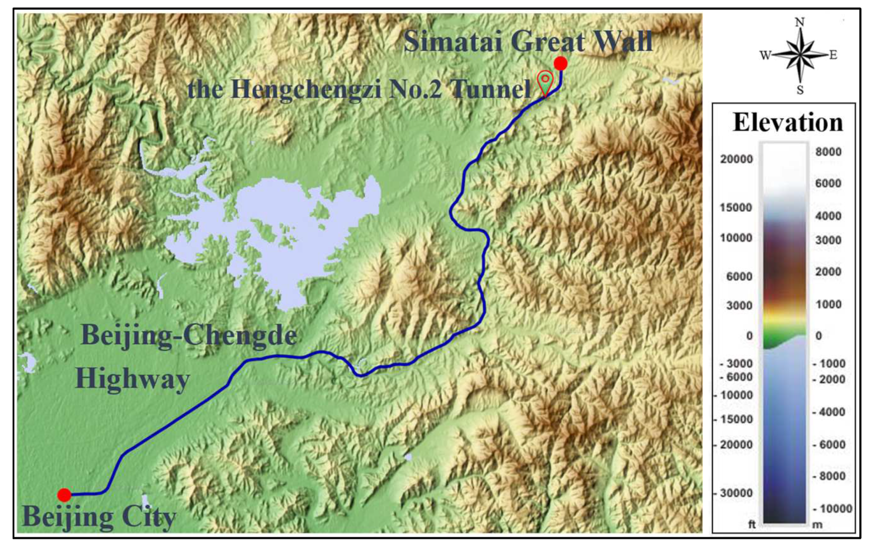
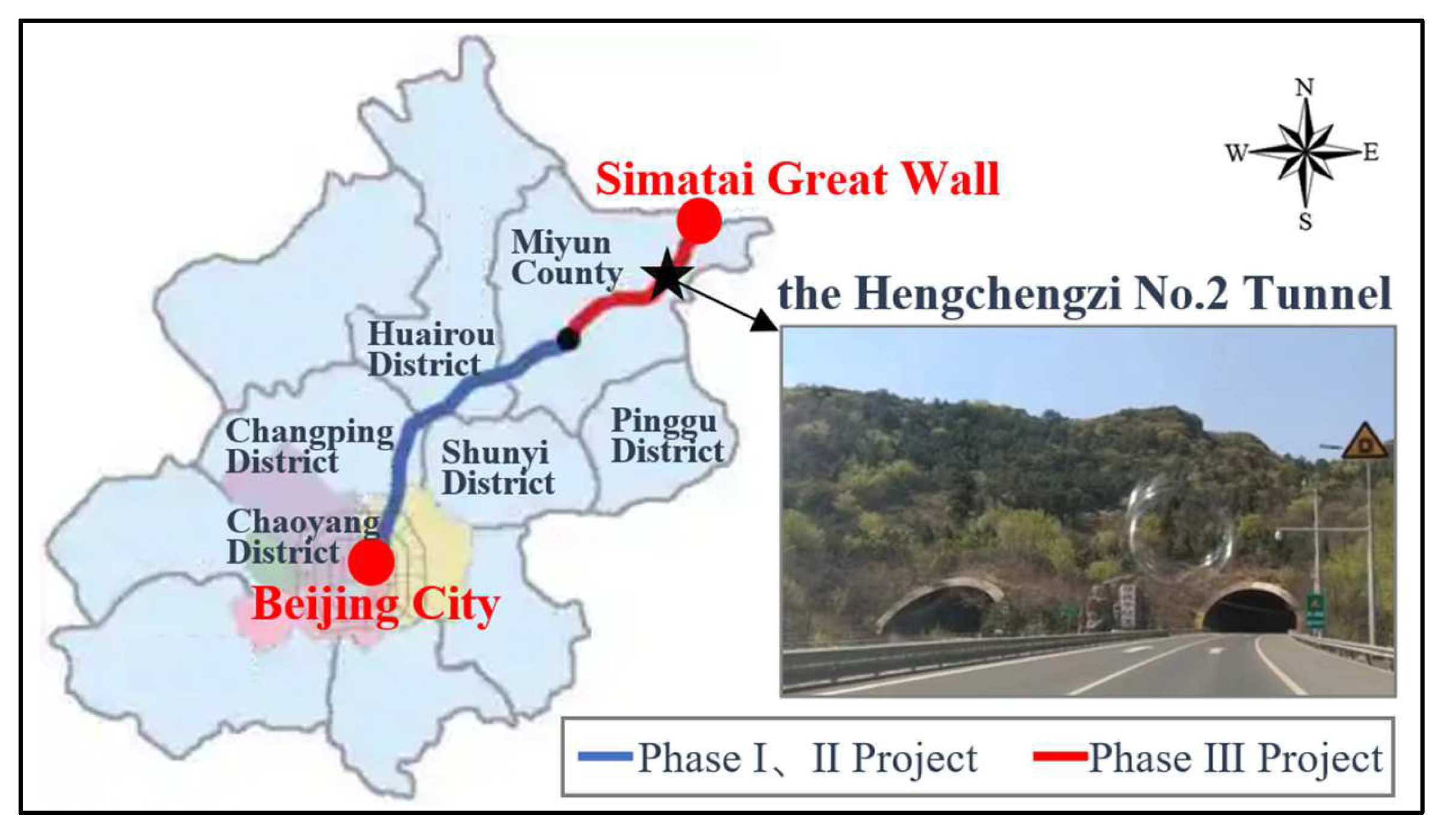
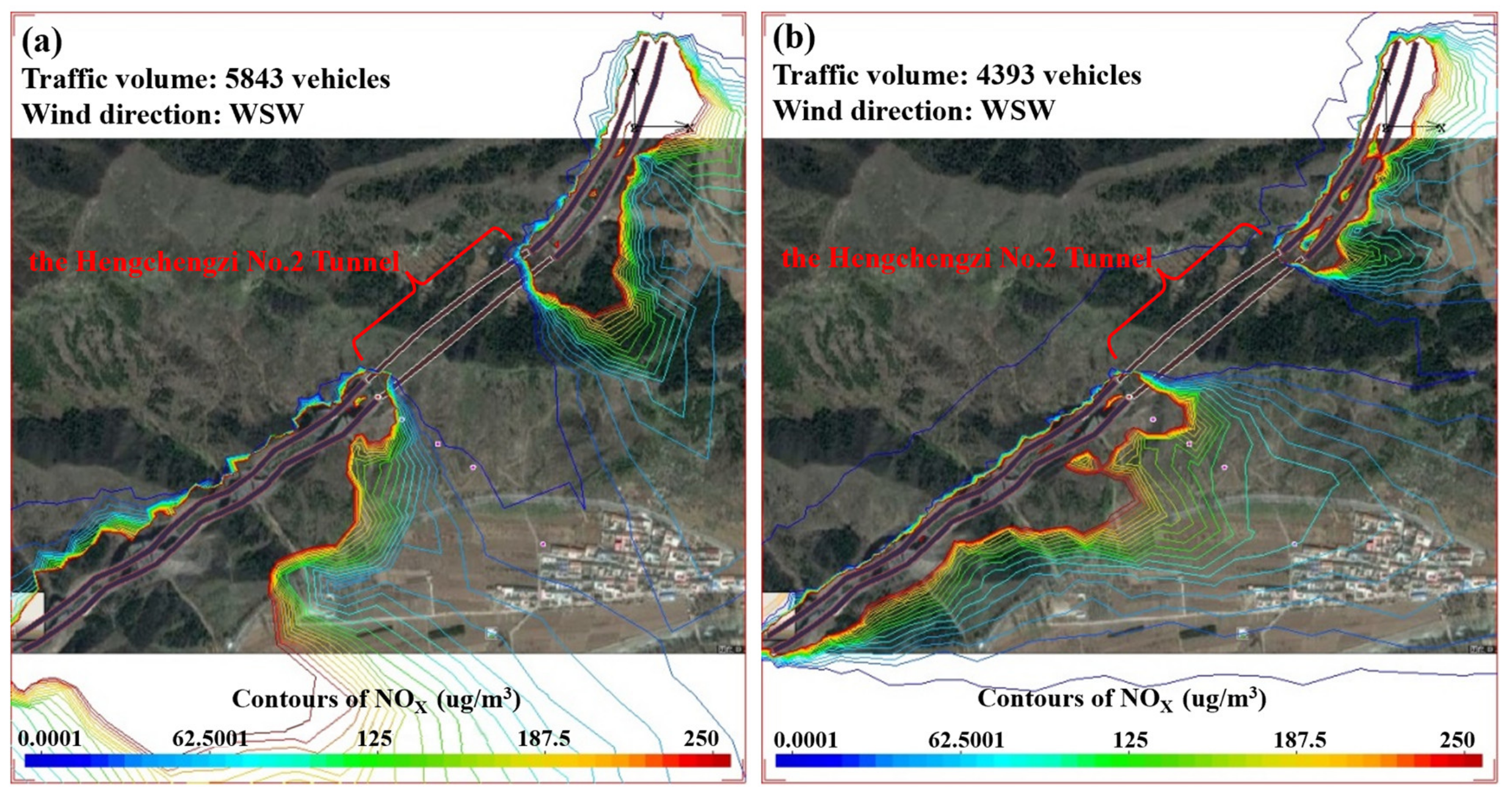
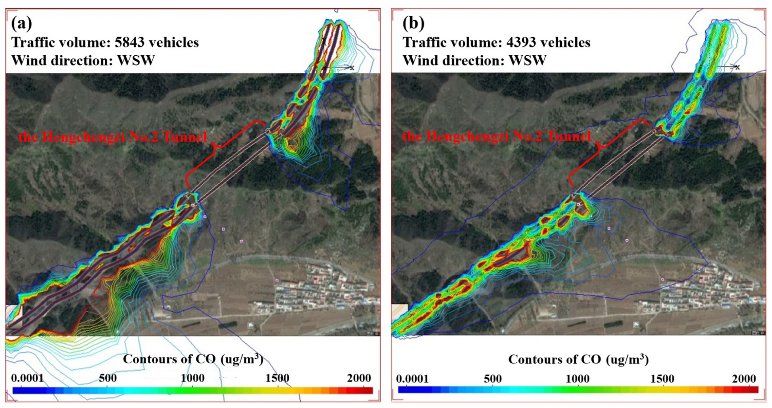
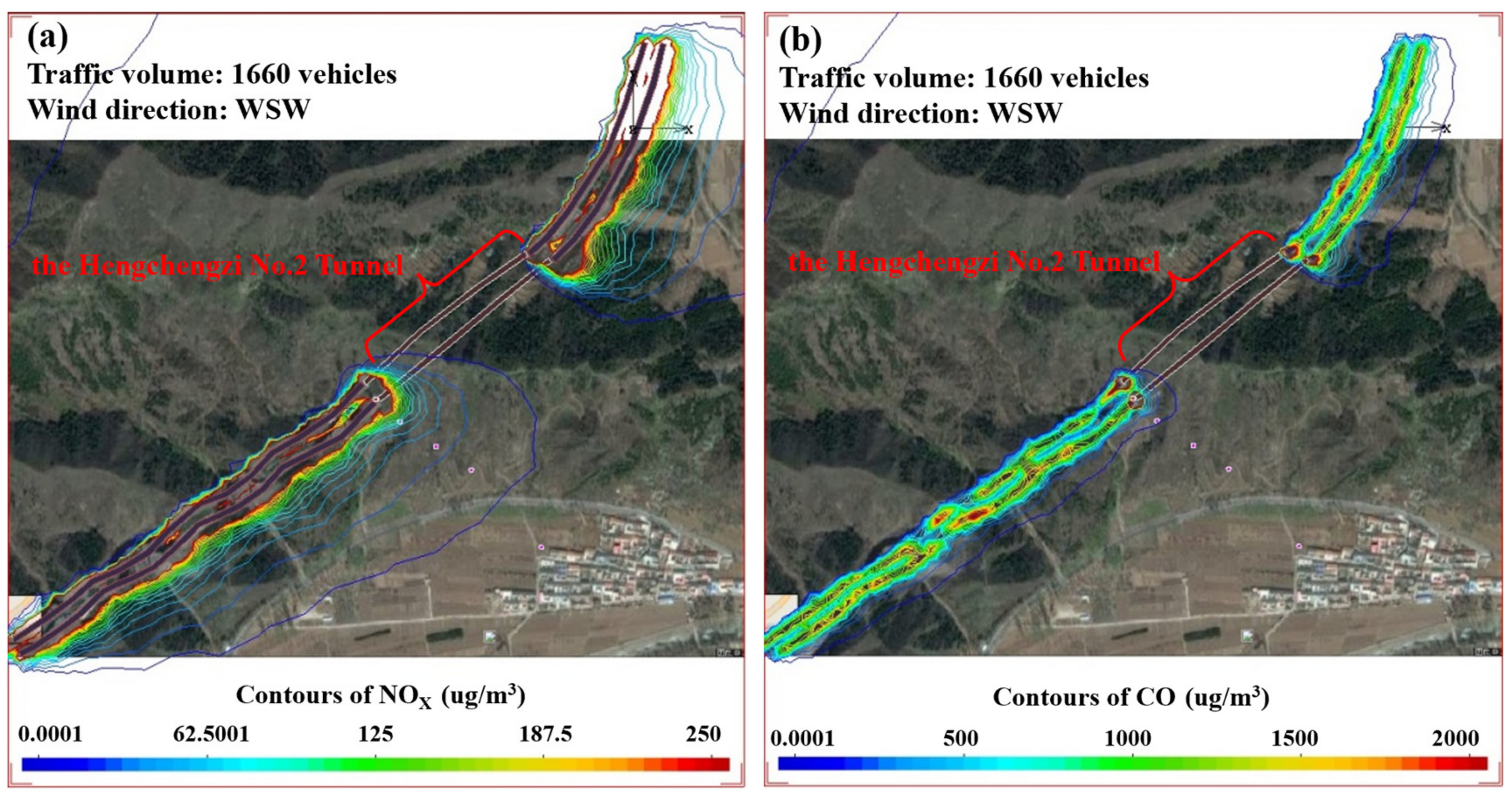
As shown in Figure 1, this paper is based on the computational fluid dynamics (CFD) model for the post-assessment of the atmospheric environment impact of the Beijing–Chengde Expressway construction project. It selects the main pollution factors NOx and CO of highway traffic for transmission and diffusion simulation analysis and prediction. It establishes the evaluation system of pollution factors in the semi-closed tunnel section under the four evaluation indicators of traffic function, environmental impact, meteorological conditions, and landform. The research conclusion clarifies the main impact factors and diffusion laws of air pollution in the complex road environment, provides a theoretical basis and technical means for promoting the quantitative work of highway atmospheric environment impact post-assessment, and then puts forward corresponding prevention and control measures and planning suggestions to promote the coordinated and sustainable development of highway construction and environmental protection.

2. Methodology

2.1. Study Area

The Beijing–Chengde Expressway is an essential part of the Daqing-Guangzhou Expressway (G45) in the National Highway Network Plan. The Beijing section of the expressway (S11) was opened to traffic on 27 September 2009, at a design speed of 80 km/h. It is not only a transit traffic channel but also a trunk road for regional traffic because it directly connects Chaoyang, Shunyi, Huairou, and Miyun districts and counties. It also indirectly connects Changping and Pinggu districts and counties. For the last ten years in Beijing, the most difficult project in terms of the survey, design, and construction of expressways was the Beijing–Chengde Expressway phase III project, which took two years to build. It is also the longest mountain expressway in Beijing. There are 8 interchanges, 108 bridges, 20 tunnels, some villages and towns along the line, and the tunnel crossing the Simatai ancient Great Wall scenic area is 2.2 km long. Therefore, it is significant in transportation, tourism, ecology, scientific research, and other aspects. According to the distribution of roadside residents and the airflow characteristics of the tunnel, this study selected the Hengchengzi No. 2 Tunnel of the Beijing–Chengde Expressway (Miyunsha Canyon–Shijie section) as the simulation and analysis objects of the atmospheric environment, as shown in

Table 1. Detailed conditions of the typical section of the study case.

Serial Number	Location	Mileage Pile Number	Longitude	Latitude	More
1	The Hengchengzi No. 2 Tunnel	K125 + 375	117.2497	40.6213	525 m and 627 m from the Xiazhuangzi and Laowa village, respectively

and Figure 2 in detail.

2.2. Simulation Methods

2.2.1. Governing Equations

The basic solution equation of Fluidyn-PANACHE [32] is the Navier–Stokes equation. Simultaneously, species concentration, mass, and energy conservation equations are solved. For the diffusion of particles and aerosols, it is also necessary to solve the equation of particle trajectories described by Lagrange. For turbulence models, PANACHE solves the Reynolds-averaged form of the above equations. The Reynolds stress model uses the linear eddy viscosity model (LEVM) [33] equation:

(1) Conservation of species concentration

$$\frac{\partial \left(\rho y_m\right)}{\partial t}+\nabla \left(\rho U{y}_m\right)=\nabla \cdot D_m\nabla \left(y_m\right)+S_m\cdots m=\left(1,2,\cdots ,n\right)$$

(1)

(2) Continuity equation

Formula (1) sums up all species and obtains a continuity equation (mass conservation)

$$\frac{\partial \rho }{\partial t}+\nabla \left(\rho U\right)=S_{\rho }$$

(2)

(3) Navier–Stokes equation (conservation of momentum)

$$\frac{\partial \left(\rho U\right)}{\partial t}+\nabla \cdot \left(UU\right)=\nabla \cdot \tau -\nabla p+S_U$$

(3)

(4) Conservation of energy

$$C_p\left[\frac{\partial \left(\rho T\right)}{\partial t}+\nabla \cdot \left(\rho UT\right)\right]=-\nabla \cdot q+\left[\frac{\partial \rho }{\partial t}+U\cdot \nabla \rho \right]+\tau :\nabla U+S_T$$

(4)

$$\tau =\mu \stackrel{·}{\gamma }\left(\frac{2}{3}\mu -\kappa \right)\left(\nabla \cdot U\right)\delta$$

(5)

$$\stackrel{·}{\gamma }=\nabla U+{\left(\nabla U\right)}^T$$

(6)

In the formulas mentioned above, $\tau$ is the viscous stress tensor; $\rho$ is the density; $\gamma$ is the deformation rate tensor; $y_m$ is the mass fraction of species; $U$ is the velocity vector; $T$ is the temperature; $p$ is the pressure; $D_m$ is the effective diffusion coefficient of species; $\mu$ is the effective viscosity coefficient; $\kappa$ is the expansion viscosity coefficient ($\kappa$ = 0 is Stokes fluid); $\delta$ is the unit quantity; $C_p$ is the constant pressure specific heat; $q$ is the heat flux vector; $q=-k\Delta T$, $k$ is the effective heat conduction coefficient; $S_m$ represents the source term of the conservation equation of species m concentration; $S_{\rho }$ represents the source term of the continuity equation; $S_T$ is the source term of the conservation equation of energy; $S_U$ represents the source term of the conservation equation of momentum.

2.2.2. Planetary Boundary Layer (PBL) Model

The PBL is an atmospheric region near the Earth’s surface, where momentum, heat, and moisture are exchanged through turbulence [34,35]. Equations describing the larger scale of the atmosphere (Equation (3) and Equation (4)) do not take into account the interaction between the atmosphere and the surface. This interaction is manifested by turbulent motion, characterized by a small-scale sub-grid, so it needs to be parameterized (modeling). The proprietary PBL model is not only built into Fluidyn-PANACHE software but also can take into account all topographic effects, such as topographic fluctuations, vegetation canopy, and urban canopy.

The PBL model, which is used to establish the interface between meteorological observations and boundary conditions required by the CFD solver, consists of two parts:

(1) Micrometeorological models: PBL basic physical parameters are calculated from observed data;

(2) The boundary layer model specifies wind speed, temperature, and turbulence vertical profiles.

2.2.3. Turbulence Model

In this study, the $k-\epsilon$ model is chosen, which is the linear eddy viscosity model of the two equations. PANACHE uses the standard Reynolds number scheme, which modifies buoyancy and compressibility to solve the transport equation of turbulent energy $k$ and its dissipation rate ε equation [36]:

$$\frac{\partial \left(\rho k\right)}{\partial t}+\left(\rho Uk\right)=\nabla \cdot \left({\mu }_t+\frac{{\mu }_t}{{\sigma }_k}\right)\nabla k+P_k+P_b-\rho \epsilon -\frac{2}{3}\rho k\nabla \cdot U+S_k^{\epsilon }$$

(7)

In the said formula,$P_k={\mu }_t\stackrel{·}{\gamma }:\nabla U$ is the mechanical generation rate of $k$; $P_b={\mu }_t\beta \frac{g\cdot \nabla T}{{\sigma }_h}$ is the buoyancy generation rate of $k$; $\epsilon$ is the dissipation rate of $k$; ${\sigma }_k=1.0$ is the turbulent dissipation Prandtl number of $k$; $S_k^{\epsilon }$ is the source term because of the vegetation canopy.

$$\frac{\partial \left(\rho \epsilon \right)}{\partial t}+\left(\rho U\epsilon \right)=\nabla \cdot \left({\mu }_t+\frac{{\mu }_t}{{\sigma }_{\epsilon }}\right)\nabla \epsilon +\frac{\epsilon }{k}\left[C_{\epsilon 1}\left(P_k+P_b\right)-C_{\epsilon 2}\rho \epsilon \right]-\left(\frac{2}{3}{C}_{\epsilon 1}-C_{\epsilon 3}\right)\rho \epsilon \nabla \cdot U+S_k^{\epsilon }$$

(8)

The $k-\epsilon$ model calculates the length of vortex turbulence fluctuations from local turbulence characteristics, so it is suitable for mechanical shear (obstacles, topographic relief, crown) and buoyancy (stability and buoyancy/heavy air). In addition, the $k-\epsilon$ model is also a turbulent isotropic model; the results calculated from it are the same in both horizontal and vertical directions.

2.2.4. Boundary Condition

When solving Equations (1)–(4), (7), and (8), the boundary conditions of the main region, the ground, and the obstacles need to be given. Furthermore, the boundary conditions are divided into three categories, as shown in

Table 2. Boundary conditions.

Types	Instruction	Given Variable	Solving Variable
Entrance	directional airflow	$U,y_m,T,k,\epsilon$	$p$
Exit	directional outflow	$p$	$U,y_m,T,k,\epsilon$
Surface	surface or obstacle surface	$U,\epsilon$	$p,y_m,T,k$

.

The top boundary is often regarded as the outflow boundary. The lateral regional boundary is usually considered an inlet or outlet boundary according to the wind direction, as shown in Figure 3.

(1) Entrance. At the boundary of the entrance, given the velocity, temperature, species concentration, and turbulent flow variables, the pressure is calculated from the inner region, and the species concentration is set in accordance with the species background concentration. Moreover, the following variables are introduced.

The speed of the entry boundary:

$$\mu =U\cos \alpha \nu =U\sin \alpha w=0$$

(9)

In the said formula, $U$ is the wind speed at a certain height from the ground; $\alpha =-\phi -{90}^{\circ }$ is the angle between wind direction and x-axis; $\phi$ is the relative direction of the north wind. The wind speed at a certain height and entrance boundary temperature is set according to the selected vertical velocity section.

(2) Emit. Even if a boundary is set as an emit boundary, the wind can still enter the area due to obstacles or canopy effects. Therefore, PANACHE both specifies some variables and deduces some variables on the basis of it.

Table 3. Exit boundary condition.

Variable	Influx	Outflow
Pressure	Define	Define
Velocity	Deduction	Deduction
Temperature	Appoint	Deduction
Concentration	Appoint	Deduction
Turbulence	Appoint	Deduction

lists several emit boundary conditions, and the static pressure at the exit boundary is usually defined as an environmental pressure.

(3) Surface. PANACHE uses the function derived from the Navier–Stokes equations of the turbulent boundary layer under equilibrium conditions to calculate the drag force on the solid wall in the turbulent boundary layer.

2.2.5. CFD Solver

PANACHE is a simulation tool that can solve nonlinear partial differential equations such as mass conservation law, momentum, energy, and various concentrations. Furthermore, the CFD solver of PANACHE solves the governing equations in three-dimensional space and time (Equations (1)–(4), (7), and (8)). These governing equations can be expressed as convection–diffusion equations with the following general forms:

$$\begin{gathered} \frac{\partial \left(\rho \varphi \right)}{\partial t}+\nabla \cdot \left(\rho U\varphi \right)=\nabla \cdot \left({\mathsf{\Gamma }}_{\varphi }\nabla \varphi \right)+S_{\varphi } \\ (\mathrm{I})(\mathrm{II})(\mathrm{II})(\mathrm{IV}) \end{gathered}$$

(10)

In the said formula, $\varphi$ is an unknown variable (momentum, temperature, concentration, etc.); ${\mathsf{\Gamma }}_{\varphi }$ is the exchange coefficient of $\varphi$ (viscosity, thermal diffusivity coefficient, etc.); $S_{\varphi }$ is the source term of $\varphi$ (discharge of pollutants, etc.). (I) is the time differential, (II) is the convection, (III) is the consumption, and (IV) is the source term.

The accuracy of the numerical solution of the above type control equations depends directly on the discrete schemes adopted in the first three items. As the discrete elements become smaller (the number of elements increases), the accuracy of calculation will be improved. However, the computation cost (memory, CPU, and time) will increase as the number of elements increases. Therefore, it is necessary to balance accuracy and computational efficiency. Moreover, the differential operators in the governing equations are discretized by Taylor series expansion.

(1) Time difference. The time difference method is approximated by a discrete time series $t^n$$(n=0,1,2,\cdots )$. The time interval is $\Delta t^n=t^{n+1}-t^n$ as the time step, ${\varphi }^n$ is the difference approximation of variables $\varphi$ at time $t^n$, and the differential term $\partial \varphi /\partial t$ is approximately expressed by the first-order difference $\left({\varphi }^{n+1}-{\varphi }^n\right)/\Delta t^n$.

(2) Spatial difference. Spatial discretization is realized by a three-dimensional mesh composed of elements (control bodies). The whole balance method is adopted to ensure the local conservation of the finite difference in each unit. The velocity vector solved by PANACHE is the Navier–Stokes equation of components in the Descartes coordinate system. All variables (pressure, velocity component, temperature, concentration, turbulence, etc.) are solved in the same control quantity.

The discretization of convection terms usually determines the accuracy of the solution. The discretization of dissipation terms is based on the second-order accuracy method. When the finite volume method is used, the convection term is expressed as:

$$\nabla \cdot \left(\rho U\varphi \right)={{\displaystyle {\sum }_f\left[\left(\rho AU\cdot N\right)\varphi \right]}}_f={{\displaystyle {\sum }_f\stackrel{·}{m}}}_f{\varphi }_f$$

In the said formula, $f$ is the surface of the control body, $A$ is the acreage, $N$ is the normal vectors on the surface, $\stackrel{·}{m}$ is the mass flux across the surface and solved by the continuity equation. Therefore, the accuracy of the calculated format is determined by calculating the ${\varphi }_f$.

2.2.6. Model Parameter Setting

Since PANACHE includes built-in automatic 3D mesh generation tools, it is possible to generate finite volume meshes for calculations around obstacles and form fit meshes along undulations. Therefore, based on the Fluidyn-PANACHE software, the topographic elevation data of the research area is imported to acquire a 3-dimensional network of topographic fluctuation. In addition, considering that the emission source is the whole road, the software chooses the line source mode, and the size is neglected relative to the whole research area. The emission parameters are set according to the results of traffic investigation at experimental sites. Then the emission source intensity of exhaust gas is calculated according to the recommended value of the single vehicle emission factor in Appendix E of the code for environmental impact assessment of highway construction projects (JTG B03-2006) to obtain the pollutant emission parameters (As shown in

Table 4. Recommended values of vehicle emission factors.

Average Speed (km/h)		50.0	60.0	70.0	80.0	90.0	100.0
Car	CO	31.34	23.68	17.90	14.76	10.24	7.72
	NOX	1.77	2.37	2.96	3.71	3.85	3.99
Medium	CO	30.18	26.19	24.76	25.47	28.55	34.78
	NOX	5.40	6.30	7.20	8.30	8.80	9.30
Large	CO	5.25	4.48	4.10	4.01	4.23	4.77
	NOX	10.44	10.48	11.10	14.71	15.64	18.38

). When calculating the annual average pollutant concentration, the following methods are used: (1) according to the hourly meteorological data, a joint frequency table including atmospheric stability level, wind speed, wind direction, and occurrence probability is calculated; (2) the steady-state method is used to calculate that the occurrence probability is greater than 0.1%; (3) all the calculation results of step 2 are weighted and averaged with the probability of occurrence as the weight to obtain the annual average distribution. The surface roughness parameters are used to represent the influence of underlying barriers, which is 0. 45 m. The final roads and tunnels are all source term models of Panache software. The difference is that the internal pollutants will be released only at both ends of the tunnel.

2.3. Evaluation Index

The diffusion of traffic pollutants is mainly affected by weather conditions such as emission sources, terrain, pollution factors, and wind speed. Therefore, the main evaluation indicators of the post-assessment method of highway atmospheric environment impact are divided into four categories: traffic function indicators, environmental impact indicators, meteorological impact indicators, and landform indicators [37].

2.3.1. Traffic Function Indicators

Traffic running conditions reflect the intensity of highway emissions source, including traffic volume, vehicle speed, and the ratio of vehicle types. Using the measured traffic volume of Hengchengzi No. 2 Tunnel in May 2012 and May 2018 to forecast the traffic volume in 2023, the input value of the traffic volume of the sensitive points is determined, as shown in

Table 5. Results of estimated traffic volume in 2023.

Vehicle Types	Minivans	Medium Truck	Large Truck	Trailer	Container Car	Minibus	Large Bus	Peak Hour Coefficient
Traffic volume	8526	8032	5128	2842	927	31324	5004	0.11
Ratio	13.8%	13.0%	8.3%	4.6%	1.5%	50. 7%	8.1%

.

The sources of pollutants emitted by vehicles on highways are calculated through actual traffic volume data. According to the recommended value of emission factors for a single vehicle in Appendix E of the Code for Environmental Impact Assessment of Highway Construction Projects (JTG B03-2006) (Table 4), the intensity of the emission source is calculated.

2.3.2. Environmental Impact Indicators

The situation of automobile exhaust emission pollution factors can be reflected by these particles, including carbon monoxide (CO), nitrogen oxides (NO, NO₂), nitrous oxide (N₂O), sulfur dioxide (SO₂), hydrocarbons (benzene, benzopyrene, etc.), lead, fine particles, and ozone. The environmental impact of various pollution factors is assessed by the secondary standards of the Environmental Air Quality Standard (GB3095-2012). Through the local investigation, it is known that there is no industrial area where the air quality reaches the standard around the sensitive point, so the diffusion simulation only needs to consider the diffusion concentration. Meanwhile, the single factor evaluation method is also used to evaluate the air quality of the sensitive point. Furthermore, the evaluation factors are CO and NOx, as shown in

Table 6. Standard values of calculated results evaluation.

Pollutants	NOX (μg/m3)	CO (mg/m3)	More
Time
Annually average	50	\	GB3095-1996
24 h average	100	\
1 h average	150	\
Annually average	50	\	GB3095-2012
24 h average	100	4
1 h average	250	10

Note *: The results of 2008 were only based on the 1996 standard values for comparison with the results of the project environmental impact report. The standard value of CO does not have an annual average concentration.

.

2.3.3. Meteorological Impact Indicators

In this study, the meteorological conditions reflecting the evaluation area mainly include wind speed, turbulence, wind direction, and pressure. According to the meteorological statistics over many years along the Beijing–Chengde Expressway, the frequency of wind direction in 2008, 2010, 2012, and 2015 is shown in Figure 4. It can be seen that NE–E is the dominant wind direction every year, followed by SW–W in the meteorological data monitored by Miyunshangdianzi Meteorological Station. The annual dominant wind speed distribution range and maximum wind speed in each direction are shown in Figure 5. Among them, the annual average wind speed range of the NNE–ENE and SW–W directions is 3.0~4.9 m/s, the E–SSW and WNW–NNW directions is 0.6–1.9 m/s, and the N direction is 0~0.5 m/s. The wind speed in the ENE direction is the largest, followed by the WSW, NE, W, SW, and NNE directions. The average wind speed of each month over the years is shown in

Table 7. The average monthly wind speed for successive years.

Month	Jan	Feb	Mar	Apr	May	June	July	Aug	Sep	Oct	Nov	Dec	Average
Speed (m/s)	3.4	3.2	3.3	3.6	3.1	2.5	2.0	1.7	2.1	2.3	2.6	3.0	2.7

. The average annual wind speed is 2.7 m/s. The seasons with higher wind speeds are spring and winter, and the seasons with lower wind speeds are summer and autumn.

2.3.4. Landform Indicators

The Beijing–Chengde Expressway is in the mountainous and hilly region, with a large topographic fluctuation, significantly impacting airflow and air diffusion. It reflects the terrain and topographic characteristics of the expressway, including mountain area, hilly area, plain area, farmland area, and residential area. The topographic maps of the project area and representative section are shown in Figure 5.

3. Results and Discussion

3.1. Traffic Function Indicators

3.1.1. Pollutant Concentration Distribution in Peak Period

The traffic volume will be the largest in 2023, its pollutant emissions will be the largest, and winter in Beijing is the season of adverse diffusion of pollutants. Considering these factors, the peak traffic volume data on 1 January 2023 is used to calculate the emission of NOx and CO pollutants. The average concentration distribution is shown in Figure 6 and Figure 7.

According to Figure 6, under the most adverse meteorological conditions, the concentration of NOx pollutants in the morning and evening peaks shows a higher concentration (>260 μg/m³) due to vehicle emissions. It is significantly higher than the upper limit of the 1 h average concentration of NOx pollutants in the secondary standard of the ambient air quality standard (GB3095-2012). Under the most unfavorable meteorological conditions, the peak appears with a wide range of diffusion and great randomness due to the more significant impact of wind direction. The hourly average concentration in the peak is higher than 100 μg/m³ and NOx diffuses in most areas of the residence near the Hengchengzi No. 2 Tunnel. Therefore, the hourly average concentration distribution of NOx in the Hengchengzi No. 2 Tunnel shows many characteristics, such as high concentration, wide distribution, and greater impact by wind direction, which is not conducive to the living health of surrounding residents. Excluding natural factors, vehicle exhaust emission is the direct cause of air pollution in tunnel sections because the peak concentration of pollutants is similar to that of vehicle exhaust; that is, the influencing factor of the atmospheric highway environment is traffic volume.

According to the analysis of Figure 7, under the most adverse meteorological conditions, due to vehicle emissions, the average concentration of CO pollutants in each road section during the morning peak and evening peak hours is relatively low, which meets the air quality standard (10,000 μg/m³).

3.1.2. Pollutant Concentration Distribution in Off-Peak Period

Considering the difference in pollutant emission and diffusion under the change of traffic volume in different periods, the emission of NOx and CO pollutants is calculated based on the hourly traffic volume data in the off-peak period on 1 January 2023. The average hourly concentration distribution of NOx and CO in the off-peak period of the Hengchengzi No. 2 Tunnel is shown in Figure 8.

According to the analysis of Figure 8, under the most adverse meteorological conditions, due to vehicle emissions, the concentration of NOx (nitrogen oxide) pollutants in the off-peak period also shows a higher concentration (>260 μg/m³). It is significantly higher than the upper limit of 1 h average NOx pollutant concentration in the ambient air quality standard’s secondary standard (GB3095-2012). The hourly average concentration of CO pollutants in the off-peak period of each road section is relatively low, which meets the air quality standard (10,000 μg/m³). Therefore, from the perspective of major pollutants, the pollutant NOx significantly impacts the atmospheric environment of the highway. From the perspective of space, the distribution range of high concentrations of pollutants in the off-peak period is mainly concentrated within 200 m of the road area, the entrance, and the exit of the tunnel. Compared with the peak period, the distribution range of pollutant concentration is smaller, and the impact on residential areas is smaller. Therefore, from the comparison of pollutant concentration distribution in peak and off-peak periods under the control variables, it can be seen that traffic flow is a direct factor affecting the highway atmospheric environment.

3.2. Environmental Impact Indicators

3.2.1. Annual Average Pollutant Concentration Distribution at the Spatial-Temporal Scale

From the perspective of spatio-temporal changes, the annual average concentrations of NOx and CO, air pollutants related to road traffic, in 2012, 2018, and 2023 are simulated and predicted to change with the spatial distance of the downwind direction along the road (the angle between the road axis and the wind direction is less than 10 degrees), as shown in Figure 9.

According to the analysis of Figure 9, the annual average pollutant concentration of NOx and CO increases with time, that is, with the growth of operation time, the traffic volume increases year by year, and the vehicle exhaust emission also increases. The main difference is concentrated within 500 m of the downwind area along the road.

Secondly, the annual average NOx and CO pollutant concentrations gradually decrease with the increase of distance. The main reduction is concentrated within 240 m of the downwind area along the road. The concentration in the downwind area along the road is unchanged within the distance of 80–120 m, and the reason may be related to the roadside shelter forest. Among them, the simulation predicts that in 2023, the average annual concentration of NOx pollutants outside the range of 150 m on both sides of the downwind area along the road will meet the secondary standard of the atmospheric environmental quality standard. The annual average change of the CO pollutants concentration with the distance from the downwind area along the road is similar to that of NOx. According to relevant regulations, there is no standard value of the annual average concentration of CO, so the annual average concentration is not evaluated. However, the results of the annual average concentration of CO in each year of the road section show that its concentration is distributed 150 m away from both sides of the downwind area along the road. This is far less than the standard value of the 24 h average. Therefore, the safe distance to the roadside of the expressway should be at least 150 m. This distance should be further studied before it is used as a reference for formulating clear road traffic and planning policies.

Moreover, the concentration of pollutants at the tunnel entrance is high, and the diffusion range is wide. An increasing trend seriously endangers residents’ health and quality of life along the line. Therefore, we should pay attention to strengthening protective measures.

3.2.2. Pollutant Concentration Distribution under Seasonal Variation

Winter in Beijing is generally the season of adverse diffusion of pollutants. In order to fully quantify the changes in pollutant concentration distribution under seasonal changes, we simulate and analyze the winter and annual average NOx and CO pollutant concentration distribution in 2018, as shown in Figure 10 and Figure 11.

According to the analysis of Figure 10 and Figure 11, the diffusion of NOx and CO pollutants in the Hengchengzi No. 2 Tunnel shows the same trend with the wind direction. The average winter concentration of NOx (>100 μg/m³) is significantly higher than the annual average concentration (>50 μg/m³), and the concentration distribution range of pollutant CO with a higher concentration (>2000 μg/m³) in winter is significantly larger than the annual average concentration distribution range. The traffic volume difference between the warm and cold seasons is ≤3%. Therefore, its evident seasonal trend can be attributed to the more stable atmospheric conditions in cold winter (less vertical mixing) and the lower boundary layer height (poor vertical diffusion ability of the atmosphere). At the same time, the continuous high humidity in the process of pollutant diffusion in winter leads to the enhancement of the secondary transformation of pollutants and the continuous increase of pollutant concentration. In addition, the concentration of pollutants at the tunnel portal is higher than that in ordinary sections, so we should focus on preventing and controlling air pollution at the tunnel portal.

3.3. Meteorological Impact Indicators

3.3.1. Pollutant Concentration Distribution under the Dominant Wind Direction

The wind direction in meteorological conditions plays a vital role in ambient air pollution by directly and indirectly affecting the emission, transportation, formation, and deposition of air pollutants. In the meteorological data of 2018, the dominant wind direction is NE (northeast–east direction). Take class D stability and 1.5 m/s wind speed to calculate the pollutant concentration distribution under the dominant wind direction. Its concentration distribution is shown in Figure 12.

According to the calculation results under the prevailing wind direction, the concentration distribution of NOx in the Hengchengzi No. 2 Tunnel section exceeds the annual average concentration standard value at 200 m on both sides of the road. The concentration of CO pollutants in the Hengchengzi No. 2 Tunnel section meets the air quality standard. However, the concentration of pollutants at the tunnel entrance is relatively high and tends to diffuse. Therefore, the results confirm the critical role of wind direction in the impact assessment of the atmospheric highway environment. It can be used to improve the understanding of the mechanism of air pollution, improve the accuracy of air pollution prediction under different meteorological conditions, and provide effective measures to alleviate pollution.

3.3.2. Pollutant Concentration Distribution under Wind Speed Change

Wind speed is an essential factor affecting the dilution and transportation of air pollutants, which is used to measure the diffusion rate of air pollutants. The pollutant concentration distribution under low (0.5 m/s), medium (2.7 m/s, average wind speed for each month over the years), and high wind speed (6 m/s, yearly maximum wind speed in all directions) changes are shown in Figure 13 and Figure 14.

Figure 13 and Figure 14 show that NOx and CO diffusion have the same change trend with the wind direction and the diffusion concentration changes with the wind speed. When the wind speed is high, the pollutant dilution ability is stronger, and the terrain fluctuation of the Hengchengzi No. 2 Tunnel section is large, resulting in stronger turbulence movement, faster concentration diffusion, and less impact on residential areas. On the contrary, when the wind speed is low, the pollutants are easier to gather, and the dilution effect is relatively not obvious; it has a significant impact on residential areas.

3.3.3. Pollutant Concentration Distribution under Temperature Change

Temperature is not only an independent factor that affects the formation and diffusion of air pollution but also an inducement of other seasonal factors (such as photochemical activities). Controlling the influence of other factors, the concentration diffusion of NOx and CO pollutants with temperature changes on a typical day in winter (1 January 2023) is predicted and simulated. Figure 15 and Figure 16 show the spatial distribution of NOx and CO throughout the study area at a low temperature (−6 °C) and high temperature (3 °C).

According to the analysis of Figure 15 and Figure 16, the diffusion range of pollutants is wide at high temperatures, and the area where the hourly average concentration of NOx pollutants does not meet the ambient air quality standards is significantly expanded. The average concentration of CO increases and changes significantly in high temperatures compared with low temperatures. Therefore, the safe distance to the roadside of the highway under high temperatures should be at least more than 400 m. The reason may be that the higher the temperature, the stronger the solar radiation, and the greater the vertical decline rate, the stronger the convective upward movement, which is more conducive to the diffusion of pollutants.

3.4. Landform Indicators

The study area is mainly a mountainous and hilly landform with large topographic relief, which runs through the Hengchengzi No. 2 Tunnel. The complex road environment has a significant impact on airflow and diffusion. The simulation predicts the pollutant concentration distribution in a favorable meteorological environment during the summer off-peak period of 2023, as shown in Figure 17.

According to Figure 17, the concentration values of pollutants NOx and CO are relatively high for the tunnel portal area and gully section. It may be because the tunnel is a semi-closed environment with only openings at both ends. Most vehicle exhaust emissions in the tunnel converge to the tunnel portal coupled with the aerodynamic effect when high-speed vehicles burst into the tunnel, resulting in the accumulation of pollutants at the tunnel portal. For the gully section, the terrain is higher on both sides, thus limiting the diffusion of air pollutants. In addition, the accumulation effect of the pollutant CO at the tunnel entrance is more pronounced, and the automobile exhaust is mainly composed of NOx (about 23%), CO (about 17%), and volatile organic compounds (VOCs > 50%) [38]. In the two-way driving tunnel, the jet exhaust at the entrance of the upstream tunnel interacts with the inlet air at the entrance of the adjacent downstream tunnel. This makes the pollutants discharged from the upstream tunnel mix into the downstream tunnel to form secondary pollution; under the interaction of inlet and exhaust air, the diffusion range and law of pollutants discharged from the tunnel are affected to a certain extent.

4. Conclusions

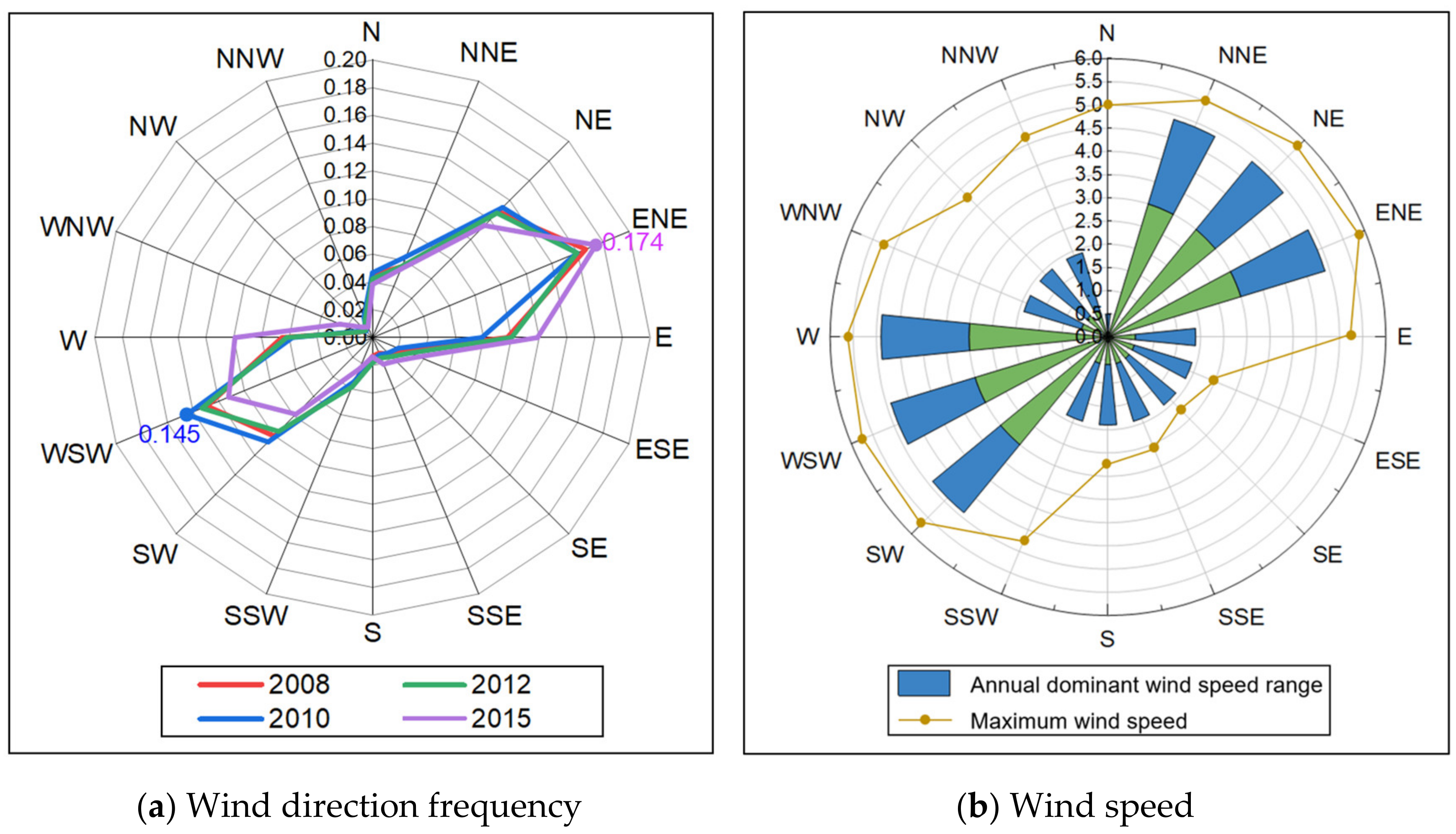
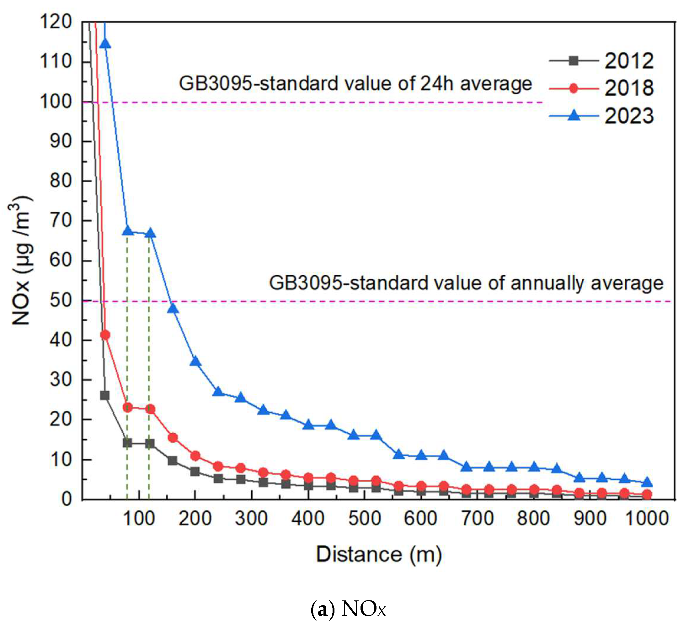
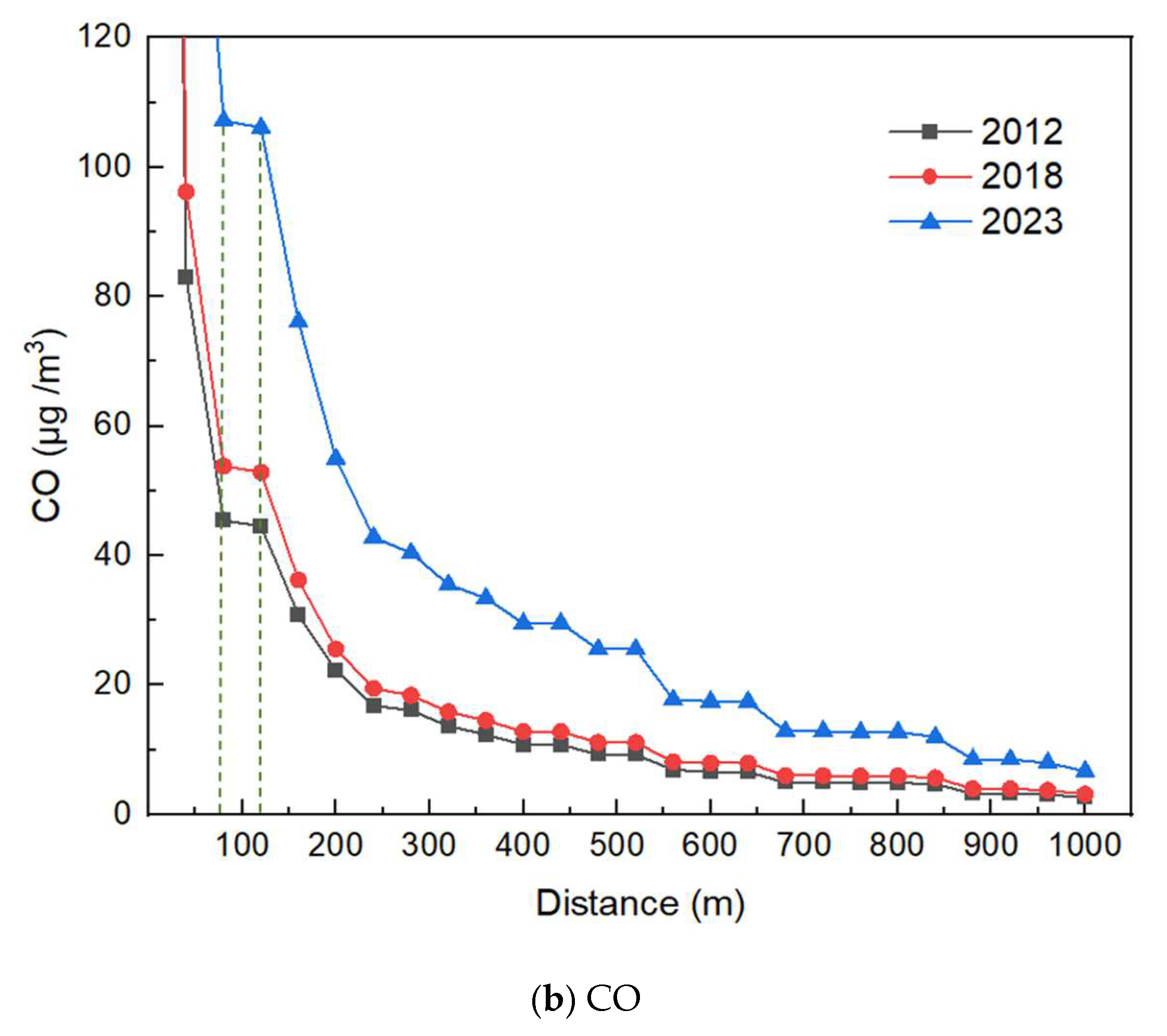
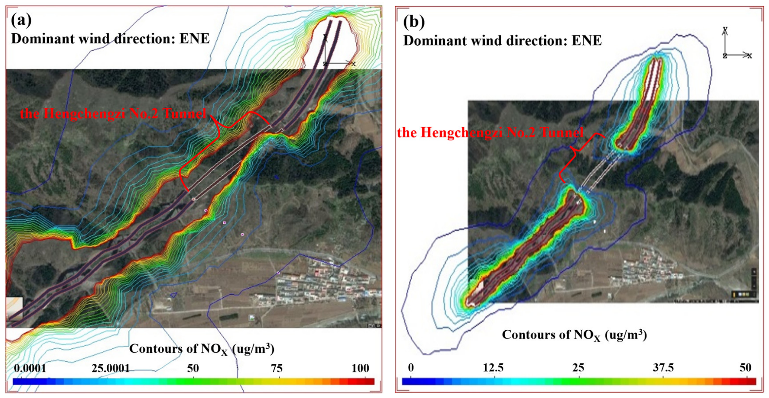
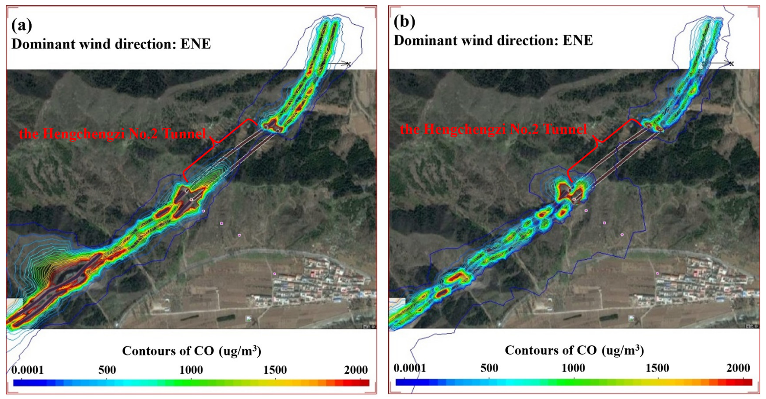
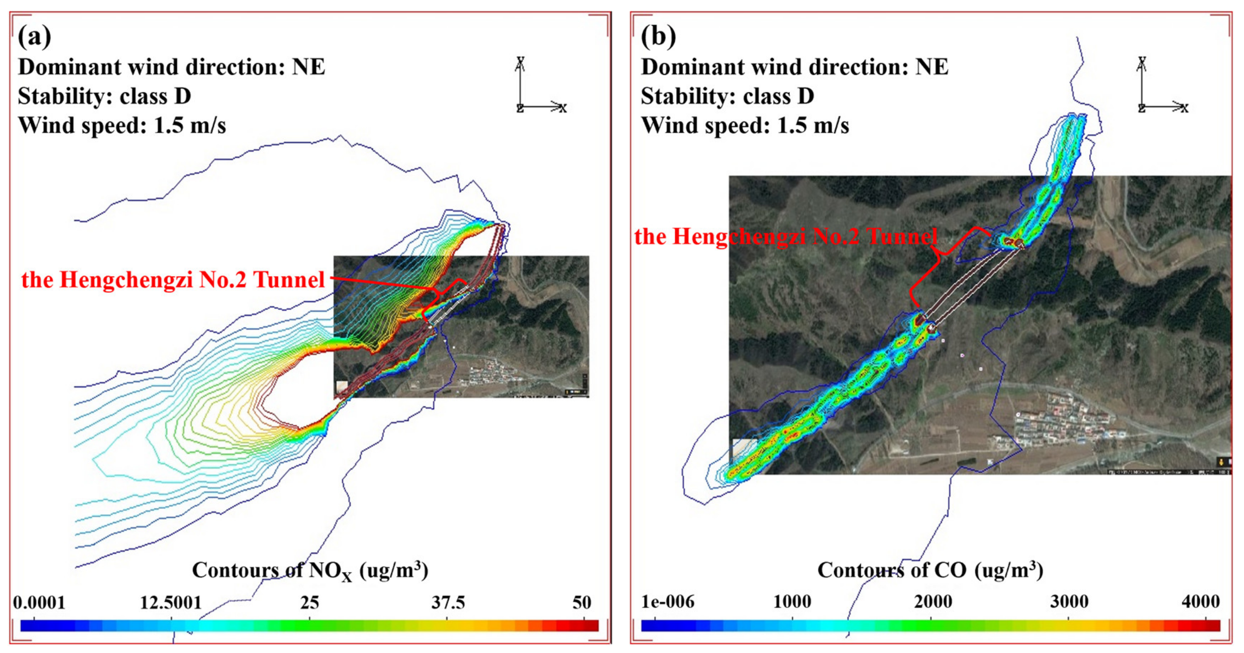
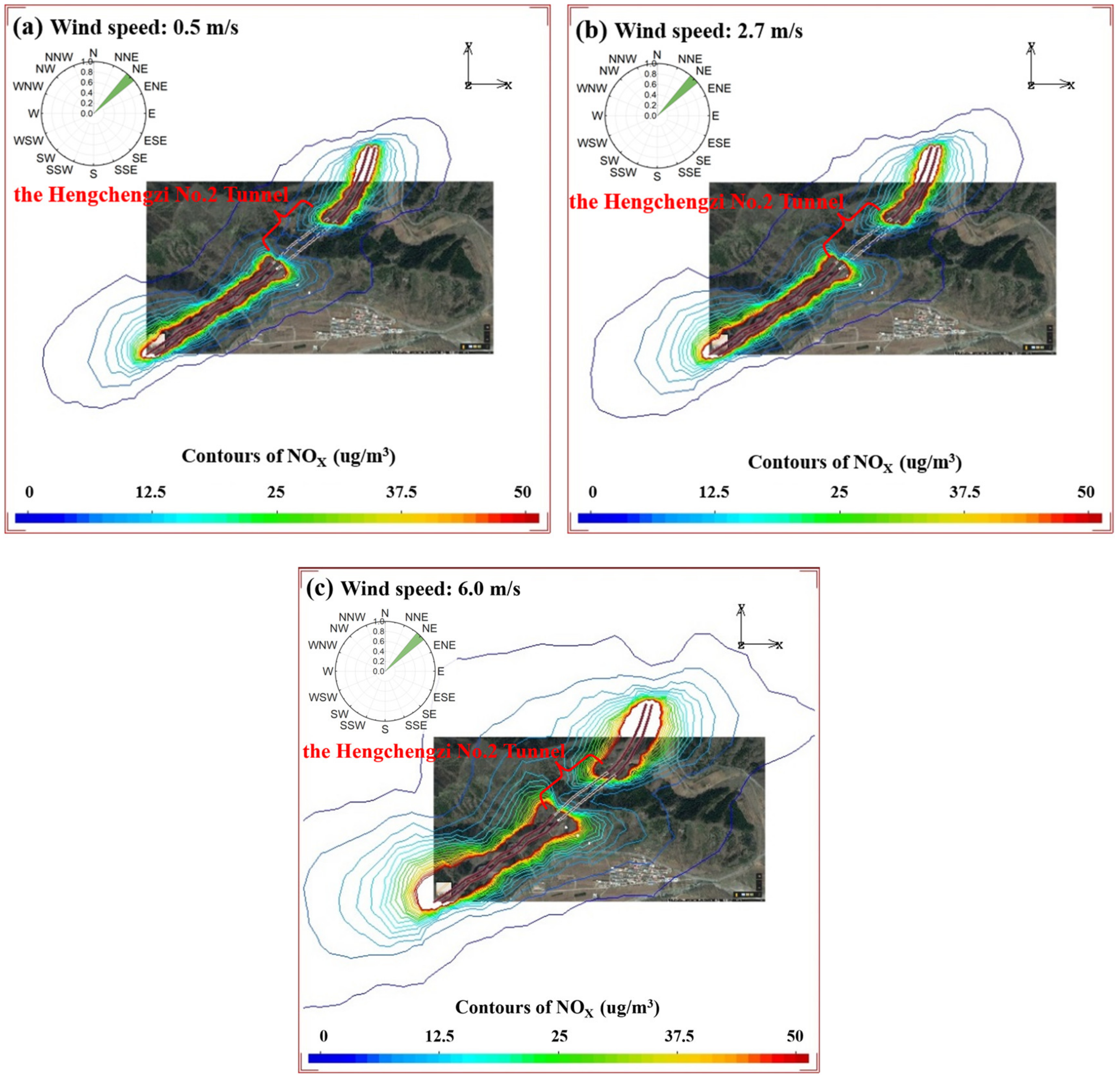
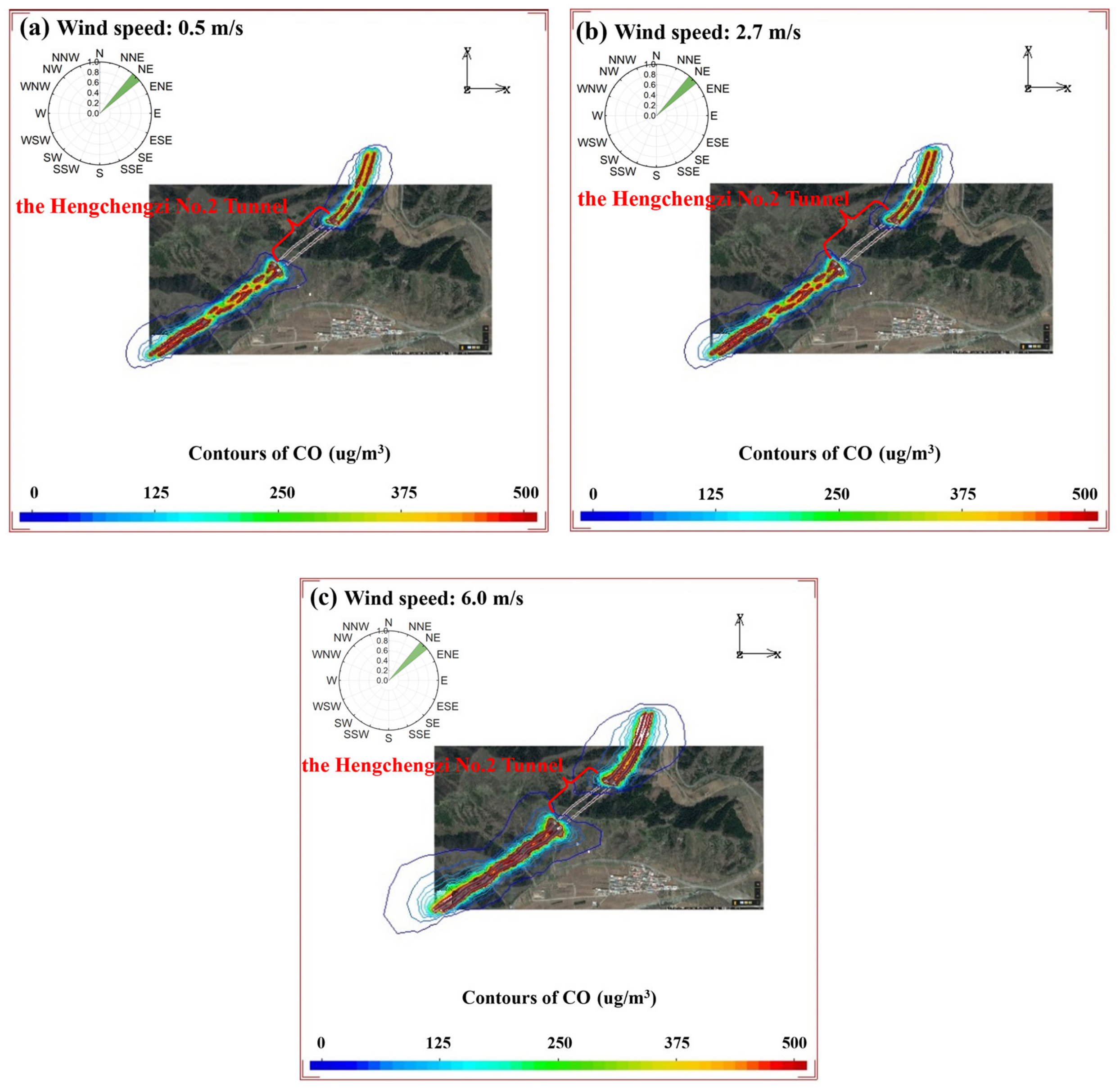
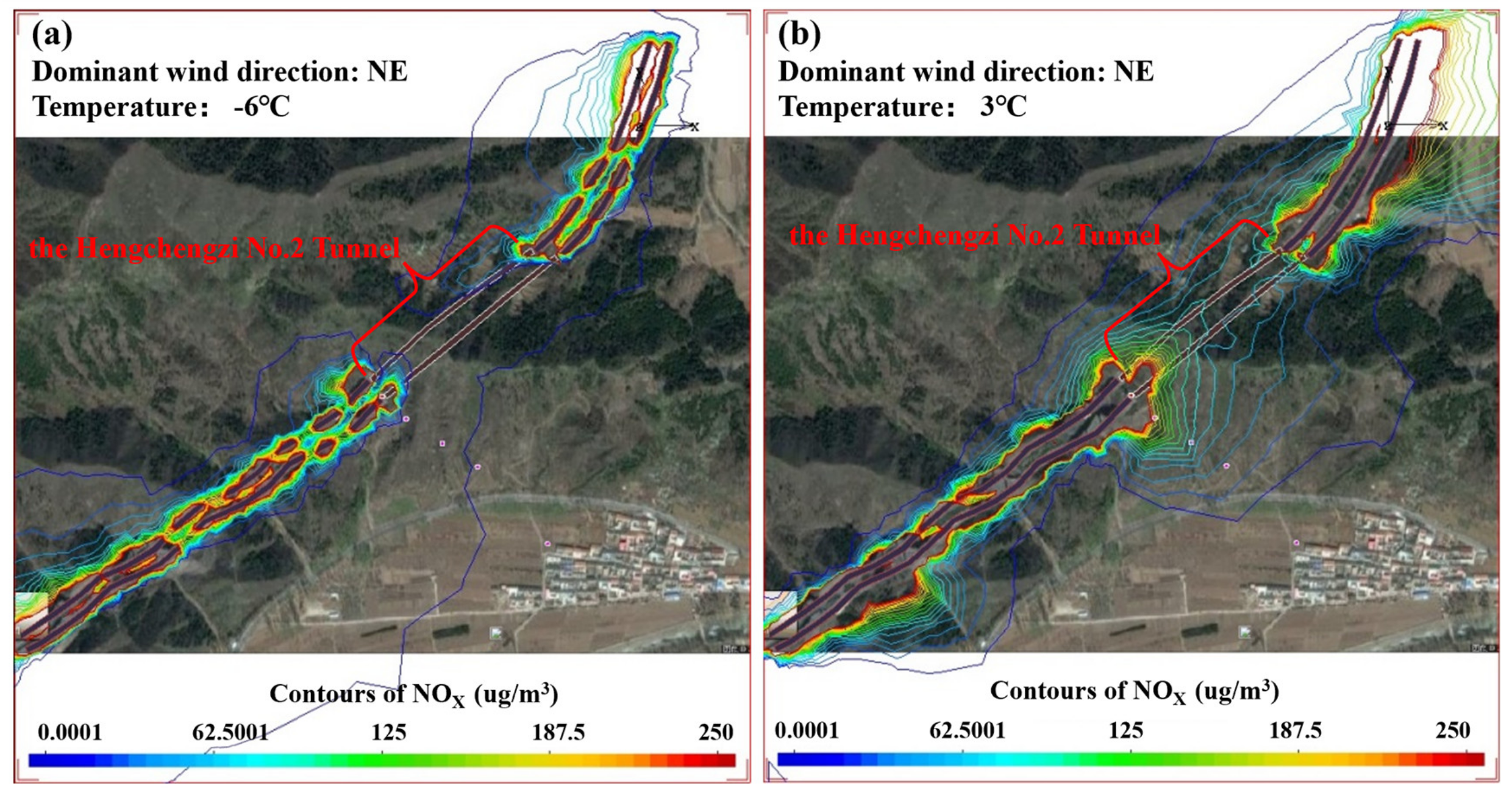
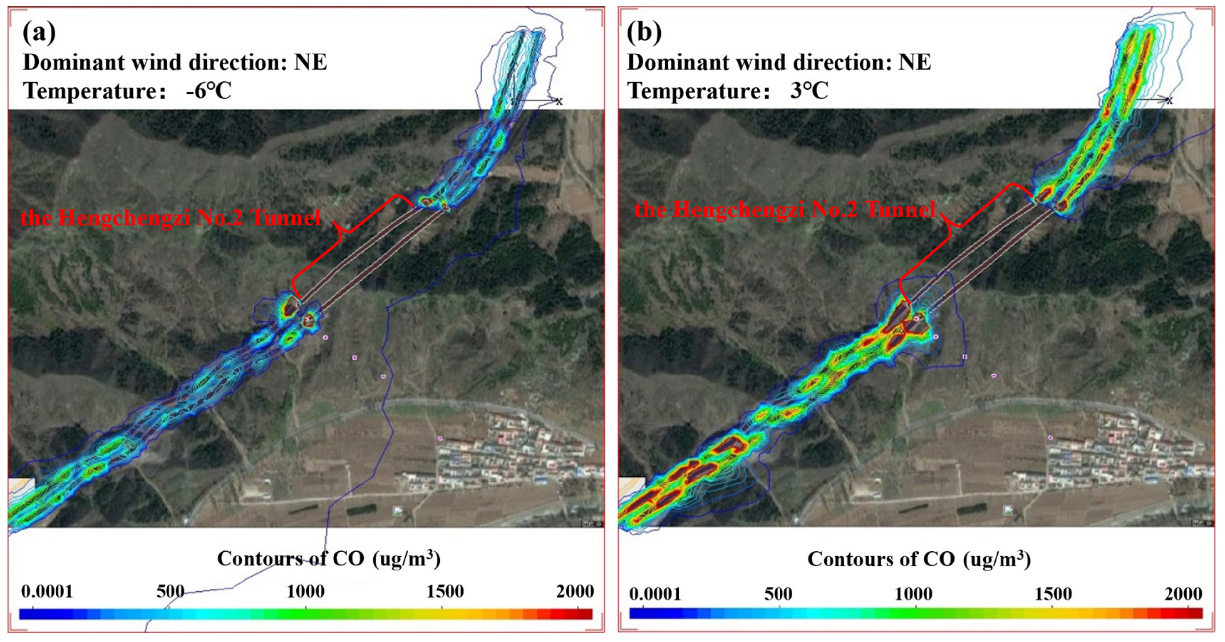
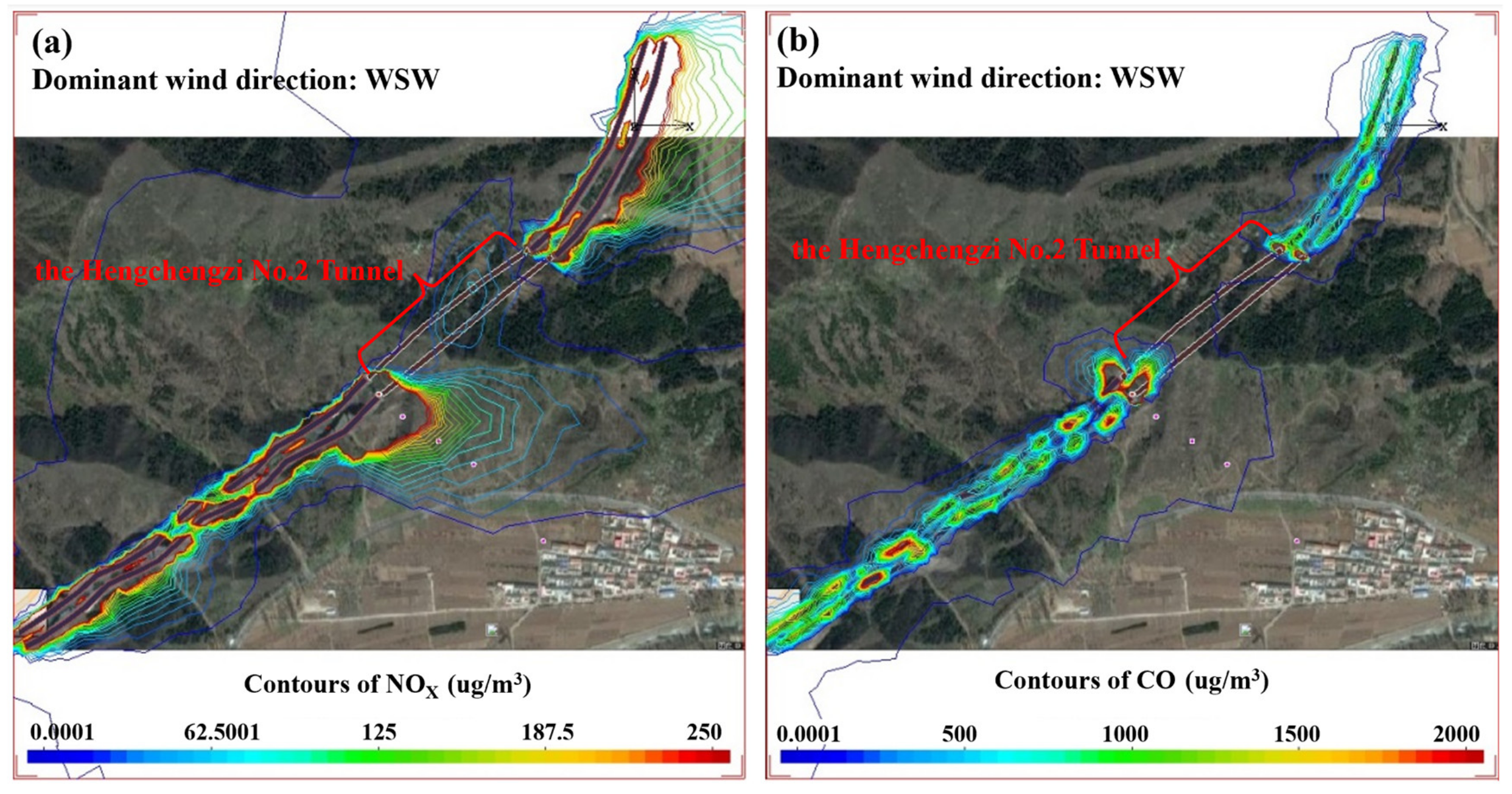
Based on the computational fluid dynamics model, this study evaluates the atmospheric environment impact of the Beijing–Chengde Expressway construction project. It systematically explores the simulation law of the transmission and diffusion of the main pollution factors NOx and CO under the four evaluation indexes of traffic function, environmental impact, meteorological conditions, and landform. The conclusions are as follows: (1) In terms of traffic functions, the intensity of highway emissions source is controlled by these factors, including traffic volume, the ratio of vehicle type, and vehicle emission factor. During the peak period, the increase in traffic flow leads to an increase in it, which makes the concentration of pollutants rise in both periods. (2) In terms of environmental impact, from the perspective of pollution factors, the concentration of NOx pollutants is generally higher than that of CO, and the environmental quality is not up to standard. In contrast, the concentration of CO pollutants in all sections and periods meets the air quality standards. From the space perspective, pollution is severe within 200 m along the Beijing–Chengde Expressway and at the tunnel portal. From the perspective of time, factors such as more stable atmospheric conditions and lower boundary layer height are not conducive to the diffusion of highway air pollutants in cold winter, resulting in relatively high concentrations of pollutants in the air. (3) In terms of meteorological impact, the higher the wind speed and the lower the temperature, the better the air is mixed into the flue gas in a unit of time. The faster the dilution, the more conducive to the diffusion of pollutants. Thus, reducing the concentration of pollutants in the air. The wind direction determines the polluted area by directly and indirectly affecting the emission, transportation, formation, and deposition of air pollutants. The pollution degree of the downwind direction is related to the wind direction frequency. Therefore, building the residential area in the downwind direction of the dominant wind direction of the pollution source is unfavorable. (4) In terms of landform, the higher the terrain on both sides, the more serious the pollution is at the gully section and the semi-closed tunnel mouth with only two openings.

Since the construction and application of the CFD model for highway atmospheric environmental impact post-assessment are still in their infancy, some theories, quantitative models, index systems, and conclusions proposed in this paper may need to be revised and should be verified by specific highway projects. Therefore, many related topics require further investigation in future research. (1) The selection of evaluation indicators to adapt to complex terrain changes and linear corridor road environment in the post-assessment system of the atmospheric environment impact of the expressway will be an insightful extension. (2) Explore the development of real-time, large-scale, and refined prediction and evaluation software of highway atmospheric environmental impact to shorten the interval between design and environmental evaluation. (3) Continue to study the post-assessment of the atmospheric environmental impact on highway tunnel sections.

References

1. Ministry of Transport of the People’s Republic of China. Statistical Bulletin of Transportation Industry Development in 2021, Beijing; Ministry of Transport of the People’s Republic of China: Beijing, China, 2022.
2. Ministry of Ecology and Environment of the People’s Republic of China. Vehicle Environment Management Anual Report, Beijing; Ministry of Ecology and Environment of the People’s Republic of China: Beijing, China, 2018.
3. Ministry of Ecological and Environmental. Annual Report on Environmental Management of Motor Source of China, Beijing; Ministry of Ecological and Environmental: Beijing, China, 2021.
4. Künzli, N.; Kaiser, R.; Medina, S.; Studnicka, M.; Chanel, O.; Filliger, P.; Herry, M.; Horak, F., Jr.; Puybonnieux-Texier, V.; Quénel, P.; et al. Public health impact of outdoor and traffic-related air pollution: A European assessment. Lancet 2000, 356, 795–801. [Google Scholar] [CrossRef]
5. Hoek, G.; Brunekreef, B.; Goldbohm, S.; Fischer, P.; van den Brandt, P.A. Association between mortality and indicators of traffic-related air pollution in the Netherlands: A cohort study. Lancet 2002, 360, 1203–1209. [Google Scholar] [CrossRef]
6. Beelen, R.; Hoek, G.; van den Brandt, P.A.; Goldbohm, R.A.; Fischer, P.; Schouten, L.J.; Armstrong, B.; Brunekreef, B. Long-term exposure to traffic-related air pollution and lung cancer risk. Epidemiology 2008, 19, 702–710. [Google Scholar] [CrossRef] [PubMed]
7. Samet, J.M. Traffic, air pollution, and health. Inhal. Toxicol. 2007, 19, 1021–1027. [Google Scholar] [CrossRef] [PubMed]
8. Weichenthal, S.; Kulka, R.; Dubeau, A.; Martin, C.; Wang, D.; Dales, R. Traffic-related air pollution and acute changes in heart rate variability and respiratory function in urban cyclists. Environ. Health Perspect. 2011, 119, 1373. [Google Scholar] [CrossRef] [PubMed]
9. Zhou, Z.-X.; Wei, H.-Q.; Zhang, H. Index system and quantized model of atmospheric environment impact post assessment for the highway. Highw. Automot. Appl. 2007, 5, 124–127. [Google Scholar]
10. Dong, W. Analysis and Simulation of the Dispersion of Atmospheric Pollutants in Urban Subsurface; Lanzhou University: Lanzhou, China, 2014. [Google Scholar]
11. Li, R.; Meng, Y.; Fu, H.; Zhang, L.; Ye, X.; Chen, J. Characteristics of the pollutant emissions in a tunnel of Shanghai on a weekday. J. Environ. Sci. 2017, 71, 136–149. [Google Scholar] [CrossRef]
12. Francis, L.; Stockwell, H. Science in the city: Monitoring air quality in the Barbican. London Mapp. Change 2017, 8, 33–34. [Google Scholar]
13. Keyte, I.J.; Albinet, A.; Harrison, R.M. On-road traffic emissions of polycyclic aromatic hydrocarbons and their oxy- and nitro-derivative compounds measured in road tunnel environments. Sci. Total. Environ. 2016, 566–567, 1131–1142. [Google Scholar] [CrossRef]
14. Kim, J.Y.; Lee, J.Y.; Kim, Y.P.; Lee, S.-B.; Jin, H.C.; Bae, G.-N. Seasonal characteristic of the gaseous and particulate PAHs at a roadside station in Seoul, Korea. Atmos. Res. 2012, 116, 142–150. [Google Scholar] [CrossRef]
15. Wingfors, H.; Sjödin, A.; Haglund, P.; Brorström-Lundén, E. Characterisation and determination of profiles of polycyclic aromatic hydrocarbons in a traffic tunnel in Gothenburg Sweden. Atmos. Environ. 2001, 35, 6361–6369. [Google Scholar] [CrossRef]
16. Grell, G.A.; Peckham, S.E.; Schmitz, R.; McKeen, S.A.; Frost, G.; Skamarock, W.C.; Eder, B. Fully coupled “online” chemistry within the WRF model. Atmos. Environ. 2005, 39, 6957–6975. [Google Scholar] [CrossRef]
17. Taseiko, O.V.; Mikhailuta, S.V.; Pitt, A.; Lezhenin, A.A.; Zakharov, Y.V. Air pollution dispersion within urban street canyons. Atmos. Environ. 2009, 43, 245–252. [Google Scholar] [CrossRef]
18. Oxley, T.; Dore, A.J.; ApSimon, H.; Hall, J.; Kryza, M. Modelling future impacts of air pollution using the multi-scale UK Integrated Assessment Model (UKIAM). Environ. Int. 2013, 61, 17–35. [Google Scholar] [CrossRef]
19. Aristodemou, E.; Boganegra, L.M.; Mottet, L. How tall buildings affect turbulent air flows and dispersion of pollution within a neighbourhood. Environ. Pollut. 2018, 233, 782–796. [Google Scholar] [CrossRef] [PubMed]
20. Tominaga, Y.; Stathopoulos, T. CFD modeling of pollution dispersion in building array: Evaluation of turbulent scalar flux modeling in RANS model using LES results. J. Wind Eng. Ind. Aerodyn. 2012, 104, 484–491. [Google Scholar] [CrossRef]
21. Lateb, M.; Meroney, R.; Yataghene, M.; Fellouah, H.; Saleh, F.; Boufadel, M. On the use of numerical modelling for near-field pollutant dispersion in urban environments−A review. Environ. Pollut. 2016, 208, 271–283. [Google Scholar] [CrossRef]
22. Meroney, R.N.; Hill, D.W.; Derickson, R.; Stroup, J.; Weber, K.; Garrett, P. CFD simulation of ventilation and smoke movement in a large military firing range. J. Wind Eng. Ind. Aerodyn. 2015, 136, 12–22. [Google Scholar] [CrossRef]
23. Kumar, P.; Feiz, A.-A.; Ngae, P.; Singh, S.K.; Issartel, J.-P. CFD simulation of short-range plume dispersion from a point release in an urban like environment. Atmos. Environ. 2015, 122, 645–656. [Google Scholar] [CrossRef]
24. Amorim, J.H.; Rodrigues, V.; Tavares, R.; Valente, J.; Borrego, C. CFD modelling of the aerodynamic effect of trees on urban air pollution dispersion. Sci. Total Environ. 2013, 461, 541–551. [Google Scholar] [CrossRef]
25. Jeanjean, A.P.; Buccolieri, R.; Eddy, J.; Monks, P.S.; Leigh, R.J. Air quality affected by trees in real street canyons: The case of Marylebone neighbourhood in central London. Urban For. Urban Green. 2017, 22, 41–53. [Google Scholar] [CrossRef]
26. Santiago, J.L.; Sanchez, B.; Quaassdorff, C.; de la Paz, D.; Martilli, A.; Martín, F.; Borge, R.; Rivas, E.; Gómez-Moreno, F.J.; Días, E.; et al. Performance evaluation of a multiscale modelling system applied to particulate matter dispersion in a real traffic hot spot in Madrid (Spain). Atmos. Pollut. Res. 2020, 11, 141–155. [Google Scholar] [CrossRef]
27. Kwak, K.H.; Baik, J.J.; Ryu, Y.H.; Lee, S.H. Urban air quality simulation in a high-rise building area using a CFD model coupled with mesoscale meteorological and chemistry-transport models. Atmos. Environ. 2015, 100, 167–177. [Google Scholar] [CrossRef]
28. Sanchez, B.; Santiago, J.L.; Martilli, A.; Martin, F.; Borge, R.; Quaassdorff, C.; de la Paz, D. Modelling NOx concentrations through CFD-RANS in an urban hot-spot using high resolution traffic emissions and meteorology from a mesoscale model. Atmos. Environ. 2017, 163, 155–165. [Google Scholar] [CrossRef]
29. Santiago, J.L.; Rivas, E.; Sanchez, B.; Buccolieri, R.; Martin, F. The impact of planting trees on NOx concentrations: The case of the Plaza de la Cruz neighborhood in Pamplona (Spain). Atmosphere 2017, 8, 131. [Google Scholar] [CrossRef]
30. Buccolieri, R.; Santiago, J.L.; Rivas, E.; Sanchez, B. Review on urban tree modelling in CFD simulations: Aerodynamic, deposition and thermal effects. Urban For. Urban Green. 2018, 31, 212–220. [Google Scholar] [CrossRef]
31. Borge, R.; Artíñano, B.; Yagüe, C.; Gomez-Moreno, F.J.; Saiz-Lopez, A.; Sastre, M.; Narros, A.; García-Nieto, D.; Benavent, N.; Maqueda, G.; et al. Application of a short term air quality action plan in Madrid (Spain) under a high-pollution episode-Part I: Diagnostic and analysis from observations. Sci. Total Environ. 2018, 635, 1561–1573. [Google Scholar] [CrossRef]
32. Fluidyn-Panache V4.0.7. 2010. Available online: http://fluent.com (accessed on 26 July 2022).
33. Reid, R.C.; Prausnitz, J.M.; Polling, B.E. The Properties of Gases and Liquids; McGraw-Hill Book Company: New York, NY, USA, 1987. [Google Scholar]
34. Stull, S.R.B. An Introduction to Boundary Layer Meteorology; Kluwer Publishers: Dordrecht, The Netherlands, 1988. [Google Scholar]
35. Banks, R.F.; Baldasano, J.M. Impact of WRF model PBL schemes on air quality simulations over Catalonia, Spain. Sci. Total Environ. 2016, 572, 98–113. [Google Scholar] [CrossRef]
36. Launder, B. Turbulence Modelling of Buoyancy-Affected Flows; Singapore Turbulence Colloquium: Manchester, UK, 2004. [Google Scholar]
37. Pasquier, A.; André, M. Considering criteria related to spatial variabilities for the assessment of air pollution from traffic. Transp. Res. Procedia 2017, 25, 3354–3369. [Google Scholar] [CrossRef]
38. Fu, X.; Wang, S.; Zhao, B.; Xing, J.; Cheng, Z.; Liu, H.; Hao, J. Emission inventory of primary pollutants and chemical speciation in 2010 for the Yangtze River Delta region, China. Atmos. Environ. 2013, 70, 39–50. [Google Scholar] [CrossRef]
Figure 1. Research route.
Atmosphere 13 01503 g001
Figure 2. The map of a typical section and the main control points of the study case.
Atmosphere 13 01503 g002
Figure 3. Flow boundary condition.
Atmosphere 13 01503 g003
Figure 4. Rose map of wind direction and wind speed.
Atmosphere 13 01503 g004
Figure 5. Topographic map of the study case.
Atmosphere 13 01503 g005
Figure 6. Hourly average concentration distribution of NOX at a peak period in the Hengchengzi No. 2 Tunnel section. (a) 7:00–8:00; (b) 17:00–18:00.
Atmosphere 13 01503 g006
Figure 7. Hourly average concentration distribution of CO at a peak period in the Hengchengzi No. 2 Tunnel section. (a) 7:00–8:00; (b) 17:00–18:00.
Atmosphere 13 01503 g007
Figure 8. Hourly average concentration distribution of NOX and CO at an off-peak period in the Hengchengzi No. 2 Tunnel section. (a) NOX; (b) CO.
Atmosphere 13 01503 g008
Figure 9. Annual average concentrations of NOX and CO vary with the distance in the Hengchengzi No. 2 Tunnel section.
Atmosphere 13 01503 g009aAtmosphere 13 01503 g009b
Figure 10. Winter and annual average concentration distribution of NOx in the Hengchengzi No. 2 Tunnel section. (a) Average concentration distribution in winter; (b) Annual average concentration distribution.
Atmosphere 13 01503 g010
Figure 11. Winter and annual average concentration distribution of CO in the Hengchengzi No. 2 Tunnel section. (a) Average concentration distribution in winter; (b) Annual average concentration distribution.
Atmosphere 13 01503 g011
Figure 12. Concentration distribution of NOX and CO under the dominant wind direction in the Hengchengzi No. 2 Tunnel section. (a) NOX; (b) CO.
Atmosphere 13 01503 g012
Figure 13. Concentration distribution of NOX under different wind speeds in the Hengchengzi No. 2 Tunnel section. (a) Low wind speed (0.5 m/s); (b) Medium wind speed (2.7 m/s); (c) High wind speed (6.0 m/s).
Atmosphere 13 01503 g013
Figure 14. Concentration distribution of CO under different wind speeds in the Hengchengzi No. 2 Tunnel section. (a) Low wind speed (0.5 m/s); (b) Medium wind speed (2.7 m/s); (c) High wind speed (6.0 m/s).
Atmosphere 13 01503 g014
Figure 15. Average concentration distribution of NOx in the Hengchengzi No. 2 Tunnel section. (a) Low temperature (−6 °C); (b) High temperature (3 °C).
Atmosphere 13 01503 g015
Figure 16. Average concentration distribution of CO in the Hengchengzi No. 2 Tunnel section. (a) Low temperature (−6 °C); (b) High temperature (3 °C).
Atmosphere 13 01503 g016
Figure 17. Concentration distribution of NOX and CO in the Hengchengzi No. 2 Tunnel section. (a) NOX; (b) CO.
Atmosphere 13 01503 g017