Analysis of Ozone Vertical Profiles over Wuyishan Region during Spring 2022 and Their Correlations with Meteorological Factors

Abstract

Understanding the vertical structure of ozone concentrations in different seasons and their correlations with the associated meteorological conditions is crucial for exploring atmospheric ozone variability and improving the accuracy of regional ozone prediction. In this study, an ozone-sounding experiment was carried out at the Shaowu sounding Station in Fujian from November 2021 to May 2022 in order to obtain vertical profiles of ozone concentrations and synoptic variables. Based on these observations, we examined the characteristics of tropospheric ozone profiles in spring over the Wuyishan region and their comparison with wintertime ozone. The results show that compared with winter, the total ozone column (TOC) in spring has increased by 64.4%, with an enhancement of 23.8% for the troposphere and a greater increment of 69.1% for the stratosphere. The sub-peaks of tropospheric ozone below 12 km are found in both spring and winter of 2022, which are accompanied by lower relative humidity (<10% in winter and <15% in spring), temperature inversions in some cases, and intensive westerly winds. Furthermore, we investigated the relationship between ozone volume mixing ratio (OVMR) and synoptic conditions in the Wuyishan region and concluded that OVMR above 1.5 km is negatively correlated with temperature and relative humidity but positively correlated with wind speed. Additionally, springtime OVMR in the middle and upper troposphere exhibits a “funnel” distribution, showing a higher OVMR on the day of sounding observations and one day before and after that on adjacent days with low-level southwesterly winds and updrafts. While in winter, the strong downdrafts dominate on the sounding observation day.

1. Introduction

Ozone (O₃) is a key trace gas in the atmosphere due to its implications for ambient air quality, atmospheric oxidation effect, stratospheric depletion, and climate change associated with greenhouse effects [1,2]. Ozone in the stratospheric serves as a protective filter that prevents the Earth from harmful ultraviolet solar radiation [3], while the tropospheric ozone is one of the dominant air pollutants that have negative consequences on human health, crop production, and climate change [3,4,5,6,7,8]. In light of the severe effect of high-concentration ozone, numerous studies were conducted to examine the distribution and variation in ground-level and total ozone [9,10] as well as its vertical structures [11,12]. Observational results show an increasing trend in surface ozone concentrations in recent decades, despite the declining concentrations of most air pollutants [13,14,15]. Specifically, some megacities of China, such as Beijing, the Yangtze River Delta (YRD), and Pearl River Delta (PRD) regions, have experienced severe ozone pollution during the past decade [16,17,18]. Seasonal and regional divergences in ozone levels have been observed. For instance, in China, winter has the lowest ozone concentration [5], whereas winter and autumn in India have the maximum ozone due to the highest amount of precursor gases [19].

In addition to the chemical components of ozone and its precursors, meteorological factors play an important role in modulating ozone concentrations and transport. Based on a long-term satellite and reanalysis dataset, Steinbrecht et al. [20] found that the global pattern of total ozone resembles the 50 hPa temperature variations, suggesting a close relationship between the two. On a regional scale, the impact of various meteorological factors on ozone concentrations has been quantified with the use of different measurements. Based on surface observations, Chen et al. [16] examined the ground-level ozone over Beijing during 2006–2016 and pointed out that among multiple meteorological factors, the temperature is the main driver for notable enhancement in summer ozone in Beijing, and such influence varies with seasons, with the stronger influence in spring and autumn. The former result has also been found in the YRD region during a heat wave episode [21]. While in winter, the mean wind speed and relative humidity exhibit the highest correlation with ozone concentrations [13]. Wang et al. (2017) suggested that strong sunlight and low wind speed are favorable to ozone generation and accumulation. Additionally, previous studies concluded that stratospheric ozone intrusion also poses noticeable influences on surface ozone pollution [22,23,24]. It was noted that surface observations provide limited insight into upper-level ozone distribution and exchange between the lower stratosphere and upper troposphere. Thus, the balloon-borne technique (ozonesondes) is widely employed to precisely measure the vertical distribution of ozone up to approximately 35–40 km [25,26] and is also used for the evaluation of satellite-based and reanalysis data [27]. Using the 2000–2019 ozonesonde observations in Hong Kong, Liao et al. [28] found that meteorological conditions, e.g., the East Asian summer monsoon, also have an important role in shaping ozone profiles. He et al. [29] utilized ozone lidar data to assess the variation in nocturnal ozone in Shaoguan city of Guangdong Province in China. This research suggests that the subtropical high and nocturnal mountain-valley breezes are responsible for the vertical transport of ozone.

Thus far, several short-term campaigns have been carried out in mainland China since the mid-1980s based on ozone-sounding measurements [16,30]. For example, Wang et al. [31] conducted a one-year (2013–2014) ozone-sounding experiment at the Kunming ozone observatory to verify ozone and temperature profiles obtained from spaceborne instruments. Such sounding observations allow us to accurately understand the interactions between meteorological factors and ozone concentrations. However, research into the climatic characteristics of ozone profiles is limited due to the lack of long-term observations within the mainland. By November 2021, six national meteorological observation stations in the mainland, i.e., Beijing, Nanjing, Hangzhou, Chongqing, Shaowu in Fujian Province, and Qingyuan in Guangdong Province (see station locations in Figure 1a), were established for the normalized operational scientific experiments of long-term observations of ozone profiles. Unlike the other sites located in urban areas, the Shaowu ozone observatory is situated on Wuyi Mountain, which has not experienced air pollution. By the end of July 2022, the Shaowu observatory successfully collected 35 ozone profiles. From 2016 to 2021, the near-surface ozone levels in Shaowu were recognized as excellent (ρ(O_3–8h) ≤ 100 µg∙m⁻³ ), accounting for 94.6%, and the proportion of good is only 5.4%. This study introduced the instruments and equipment, workflow, and detection elements used in China’s six operational experimental bases for ozone sounding observation; described the basic situation of ozone sounding observation in winter and spring of 2022; and summarized the basic characteristics of ozone partial pressure and OVMR in different seasons and compared them. Our previous study examined the distribution of wintertime ozone profiles based on ozone-sounding observations [26]. This study aimed to investigate the distribution of springtime ozone profiles and the difference between ozone in spring and winter. More importantly, we further explored how these profiles are affected by meteorological conditions, particularly within the troposphere. The findings can provide valuable insight for predicting and controlling ozone pollution in this region. This observation and basic research work are rare in China. It is of great scientific significance to preliminarily explore the vertical distribution and change trend of ozone in the troposphere and stratosphere in the low latitude clean region of China. Moreover, it has high practical value in providing strong observational evidence for revealing the synoptic diagnosis mechanism of the generation and disappearance of ozone pollution in the near-surface layer in the southeast coastal region.

2. Data and Method

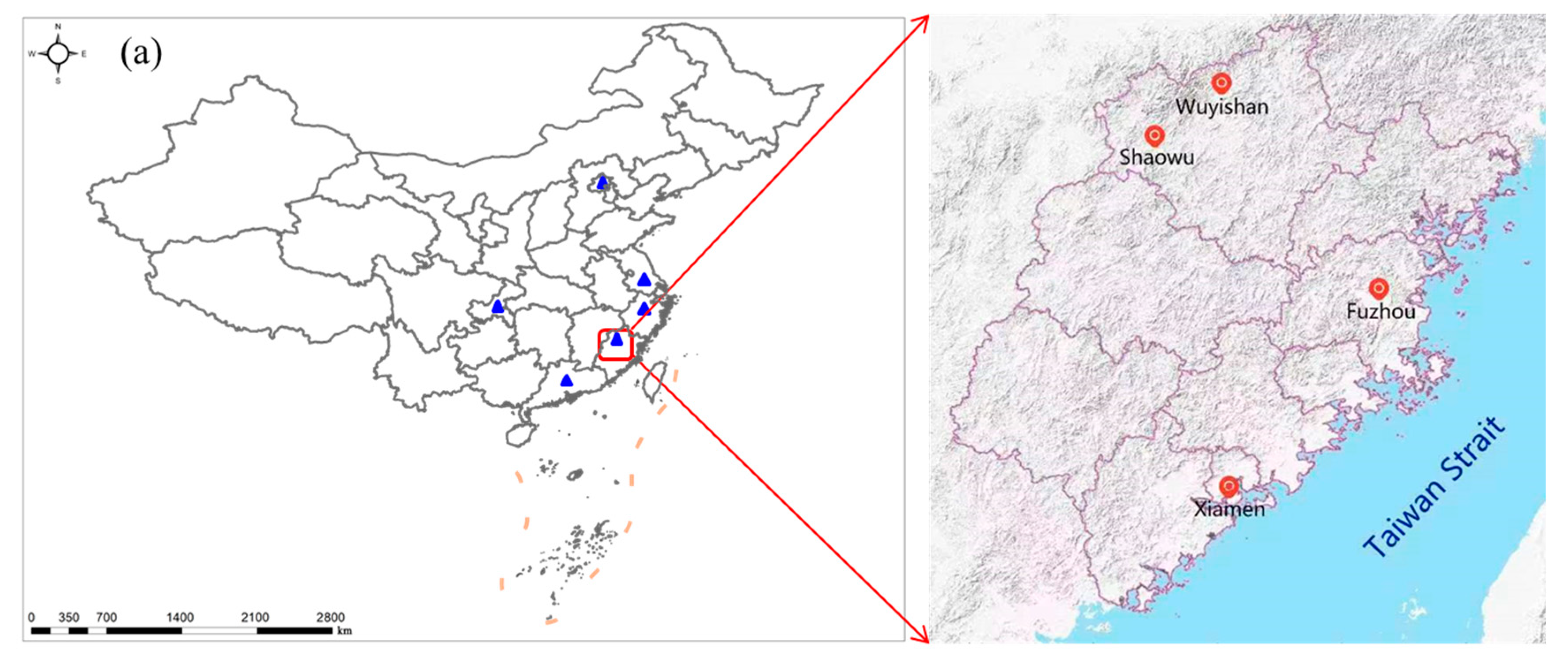
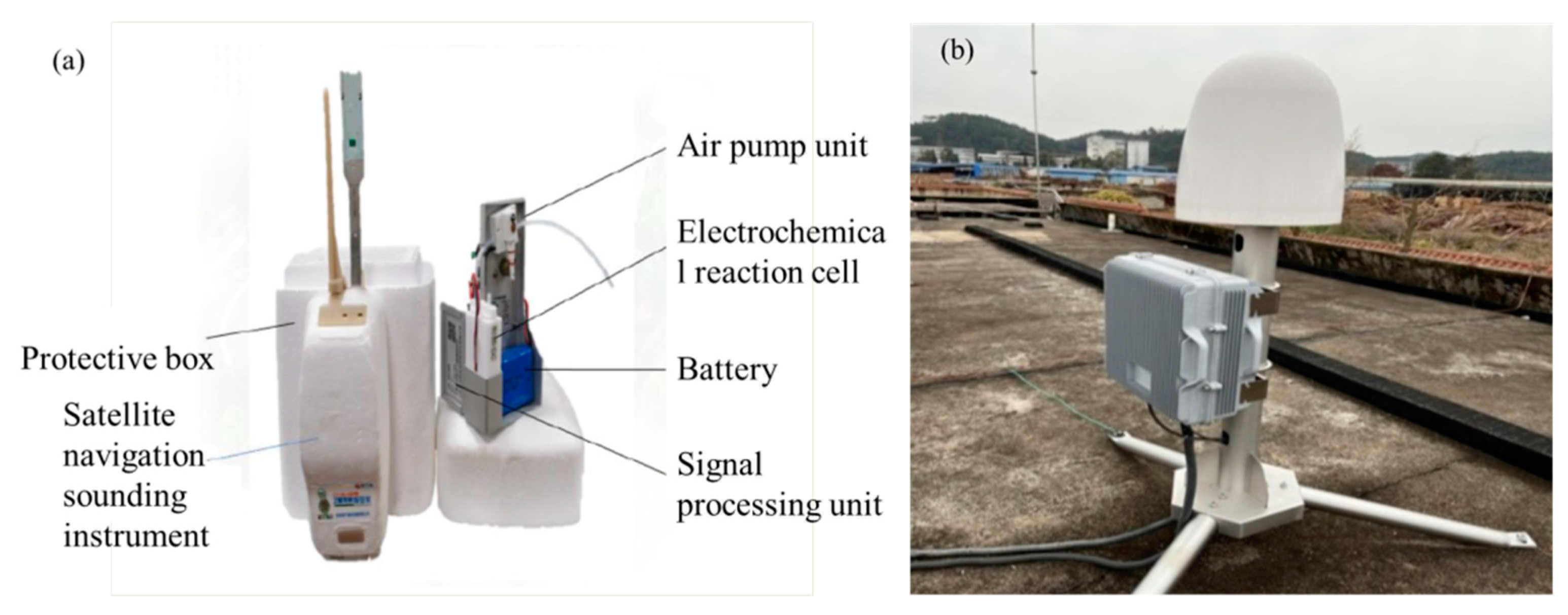
2.1. Ozone-Sounding Observation

The vertical profiles of ozone concentration and associated synoptic variables are measured by an ozone-sounding system, which is sited at the Shaowu ozone observatory (station number: 58725, 27.32° N, 117.49° E, altitude: 218.9 m) of the Wuyishan National Meteorological Observation Station. The locations of the Wuyishan and Shaowu stations are denoted by red dots in Figure 1b.

The sounding system mainly consists of an ozone sounding sensor (CTY-1, see Figure 1a) and a Beidou satellite navigator (Figure 2b). The related parameters of the measurements are well documented in Zheng et al. [26]. The ozone-sounding experiment was generally performed every Wednesday at 14:00 (Beijing Time). Otherwise, it would be postponed to the same time on Thursday or canceled when it rains on these two days. A total of 25 ozone-sounding observations, including 12 winter profiles and 13 spring profiles, were carried out from November 2021 to May 2022. The measurements of the profiles of air pressure, temperature, relative humidity, wind speed and direction, and ozone partial pressure were then retrieved for analysis.

2.2. Ozone Volume Mixing Ratio

The ozone content is expressed in two units of ozone partial pressure (units: mPa) and ozone volume mixing ratio (OVMR, units: ppb). The former is the data directly measured by ozone sounding as abovementioned, and the latter is calculated through ozone partial pressure P$o_3$ and air pressure P (units: hPa), which is expressed as:

$$OVMR=\mathrm{10,000}\times \frac{P_{O_3}}{P}$$

2.3. Total Ozone Column

Given OVMR and air pressure at each height, the total ozone column (TOC, units: DU) integrated from the near-surface (~0.2 km) up to the height of the balloon blasting point (~40 km), covering the boundary layer, troposphere, and stratosphere, can be computed from the formula as follows:

$$TOC=0.7890{{\displaystyle \int }}_{P_2}^{P_1}OVMR \left(\times {10}^{-6}\right)dP$$

2.4. Reanalysis Data

The latest fifth-generation ERA5 reanalysis dataset from the European Centre for Medium-Range Weather Forecasts (ECMWF) is used for further synoptic analysis [32]. The data set provides hourly estimates on a 0.25° × 0.25° grid and 37 pressure levels, covering the period from 1979 onwards. Here, we vertically interpolated ERA5 data with pressure levels to height levels for consistency with station observations.

3. Results

3.1. Overview of Springtime Ozone Profiles

The average maximum height of ozone sounding observations at Shaowu station is 38.1 km in spring (March to May 2022), which is 0.9 km higher than that in winter (December 2021 to February 2022, since the first ozone sounding observation in Shaowu was on 24 November 2021, the winter was just one week away, it was classified as the winter of 2022 in order to ensure the continuity of the sample). The ozonesonde launching details for the spring season are tabulated in

Table 1. Ozonesonde launching details (launching date and time) along with balloon bust height, flight time, CPH (cold point troposphere), and CPT (cold point troposphere temperature) observed in spring 2022 at Shaowu station.

Date	Launching Time	Balloon Burst Height (km)	Flight Time (Min)	CPH (km)	CPT (°C)
2 March 2022	13:17	37.9	94	17.3	−81.2
9 March 2022	13:17	38.3	101	18.2	−77.8
16 March 2022	13:21	38.6	96	17	−73.0
23 March 2022	13:15	36.7	100	17.1	−79.7
30 March 2022	13:15	37.6	114	17.6	−78.4
6 April 2022	13:15	37.8	108	17.8	−75.1
14 April 2022	13:18	38.4	107	17.7	−72.3
20 April 2022	13:16	38.4	99	18.1	−72.7
27 April 2022	13:19	39.5	113	17.4	−78.9
4 May 2022	13:38	36.4	99	17.2	−72.1
11 May 2022	13:44	37.7	95	18.1	−76.9
18 May 2022	13:27	39.6	115	16.6	−77.1
26 May 2022	13:54	38.4	98	17.4	−76.2

. Except for the observation on 2 June 2022, affected by convective weather, the detection heights of all observations reach 35 km or higher, covering the upper stratosphere, with the highest altitude being 39.6 km measured on 18 May 2022. The average flight time of the balloon is 103 min, which is 6 min longer than that in winter. The quality of sounding observations in spring was better than that in winter.

In spring 2022, the maximum ozone partial pressure was observed at roughly 25 km, ranging from 11.5 mPa to 15.8 mPa, with an average of 13.7 mPa at 24.6 km (Figure 3a). In contrast, the maximum OVMR ranges from 7857.7 ppb to 10,495.5 ppb, with an average value of 8817.3 ppb at 31.2 km (Figure 3b), which is 5.6 km higher than the average height of the maximum ozone partial pressure.

3.2. Seasonal Variations in Ozone Partial Pressure Profiles

The mean profile of ozone partial pressure exhibits a single peak at around 25 km in both spring and winter of 2022 (Figure 4a). Seasonal differences in tropospheric ozone partial pressure can be clearly seen in Figure 4b. Comparisons between the profiles in winter and spring indicate a larger ozone partial pressure in spring than in winter, especially at nearly 25 km and near the surface (Figure 4a). Quantitative results show that spring ozone partial pressure is overall 1.1 times greater than that in winter; this discrepancy decreases from the near ground towards the tropopause, reaching its maximum of 1.6 times near the surface. Ozone partial pressure increases linearly with heights in winter but is nearly constant in spring within the boundary layer (below 1.5 km), where the dispersion between the mean and individual profiles is larger than that in the free troposphere (Figure 4b).

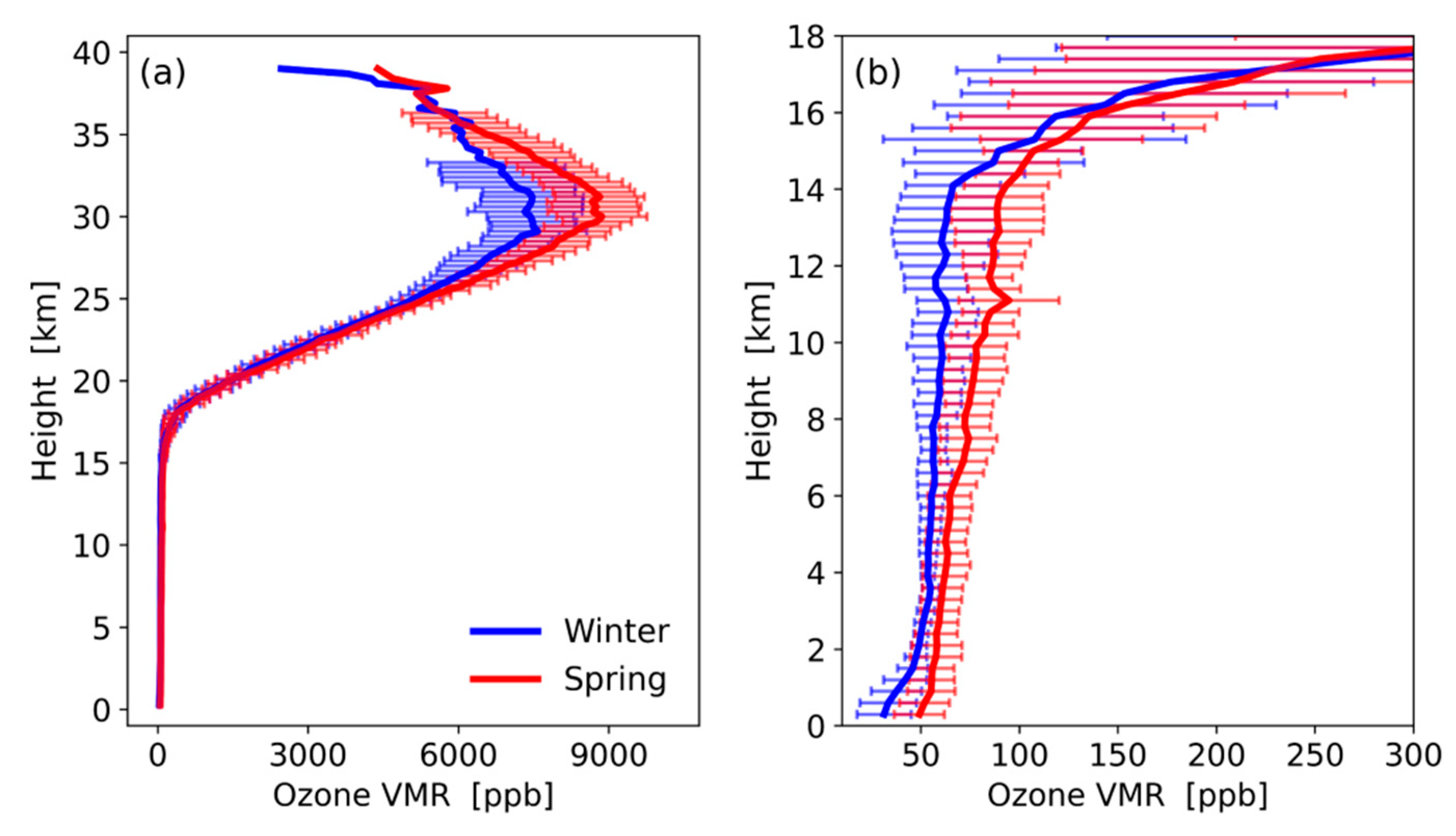
3.3. Seasonal Variations in OVMR Profiles

The average value of stratospheric OVMR in spring is remarkably higher than that in winter, with a maximum difference of 1.2 times at around 30 km (Figure 5a). The tropospheric OVMR (below 12 km) is greater in spring than in winter (Figure 5b), which is also found in other subtropical regions [28]. In particular, the seasonal difference is between 6 and 42 ppb, i.e., 1.1–1.6 times higher than in winter. Previous studies suggested that such seasonal feature of spring ozone maximum is largely due to the combined effects of stratospheric intrusion and biomass burning [28,33]. Regardless of seasons, the OVMR dispersion below 11 km is relatively small (10–16 ppb) compared to the stratosphere, where the standard deviation begins to enhance significantly with altitudes. This reflects a large and minor dispersion of stratospheric and tropospheric OVMR among the individual observations, respectively.

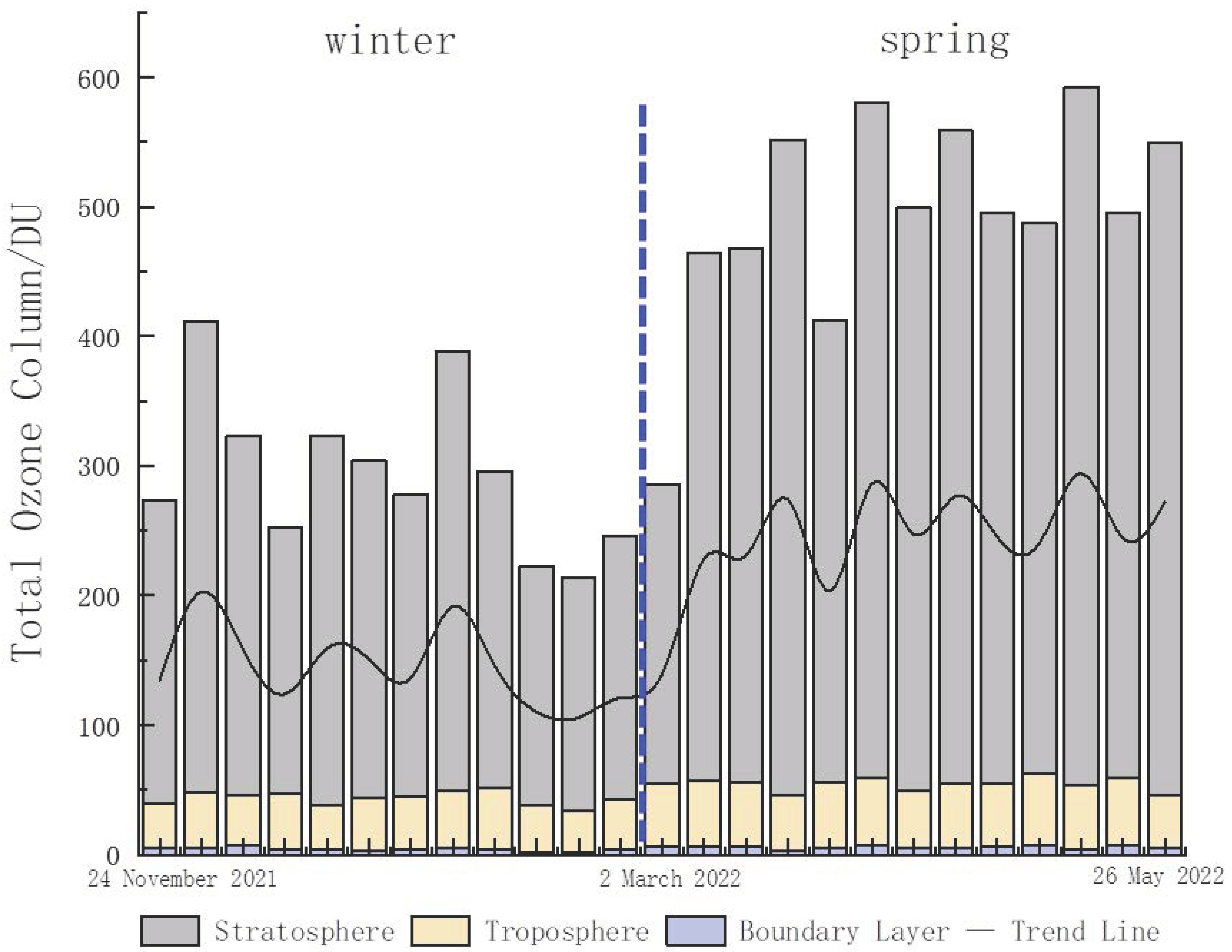
3.4. Seasonal Variations of Total Ozone Column

The TOC of spring is between 279.3 and 588.6 DU with an average of 496.3 DU (see the black line in Figure 6), which is 64.4% greater than wintertime TOC. Based on these 25 ozonesonde observations, the TOC grew significantly from November 2021 to May 2022, which is contributed mostly by a 69.1% increment in stratospheric TOC. It is also noted that the tropospheric TOC and ozone integrated over the boundary layer have risen as high as 23.8% and 37.2%, with the average value of 48.9 DU and 5.9 DU, respectively.

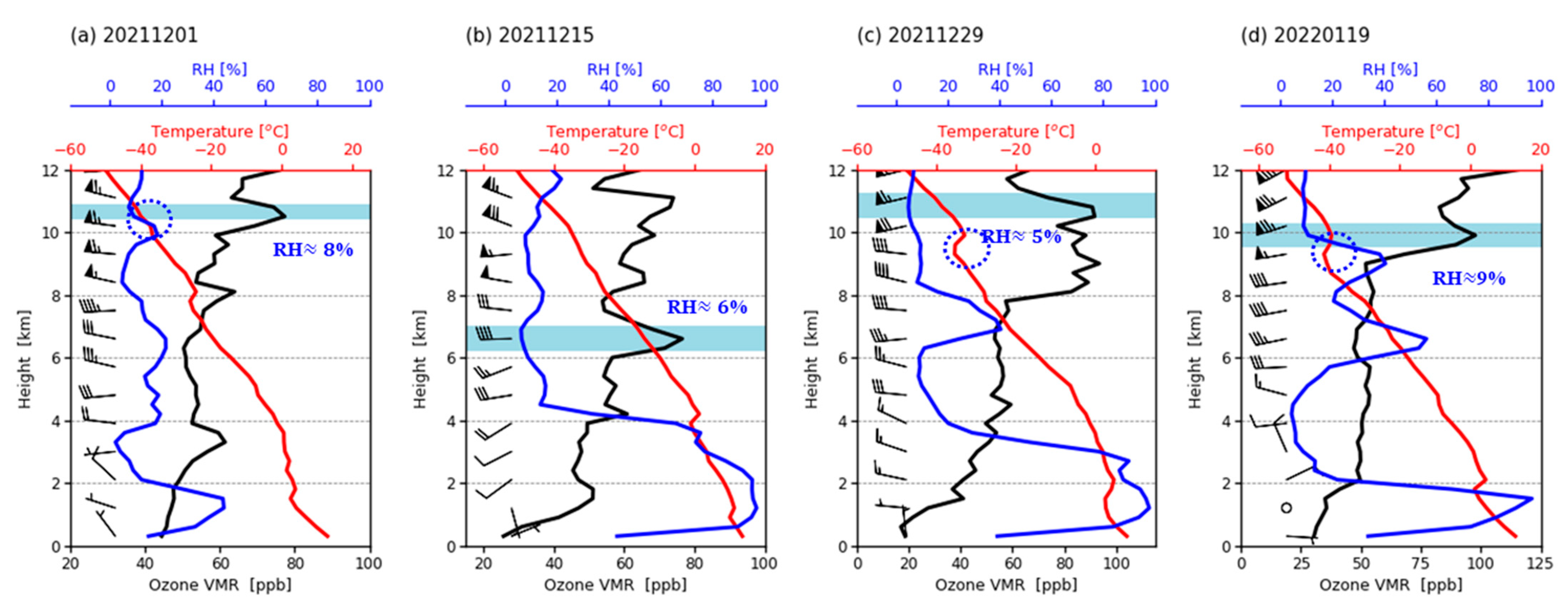
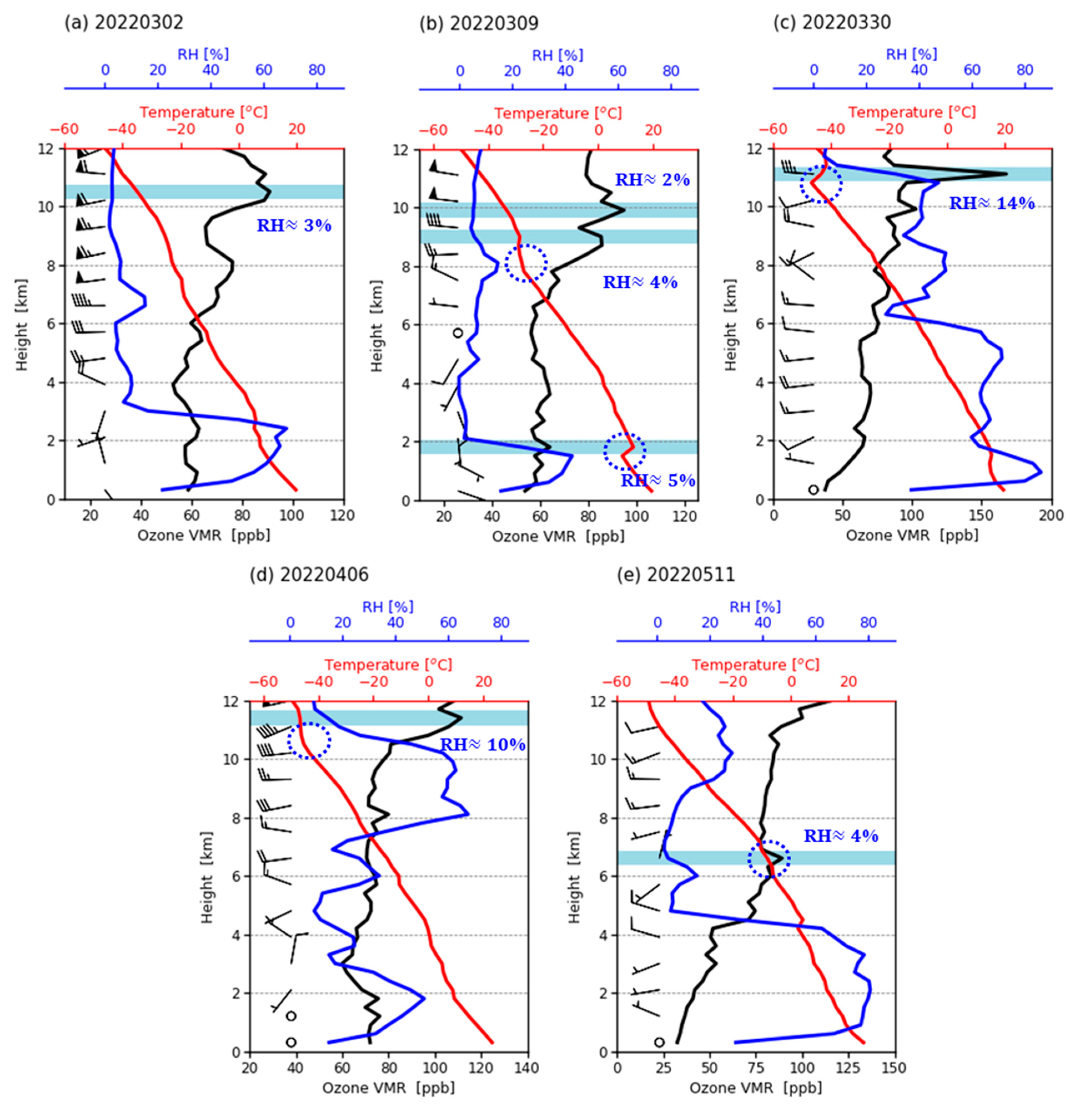
3.5. Characteristics of Tropospheric Ozone Sub-Peak

In this study, we define the ozone sub-Peak phenomenon as the OVMR variability exceeding 15 ppb/km. By definition, four out of twelve wintertime profiles show a single sub-peak at 6–12 km (Figure 7), which is 1.5–1.9 times more than the average state at the same height (see the blue line in Figure 5). The sub-peak is characterized by extremely low RH values (<10%) and strong westerly winds, as well as temperature inversions, which existed below the sub-peak height with the exception of the observation on 15 December 2021 (Figure 7a,c,d). More importantly, the inversion structure promotes the stability of sub-peaks by preventing ozone-rich air from being transported downward to lower layers [33,34]. The sub-peak phenomenon and the source of wintertime ozone are closely associated with dynamic transports of stratospheric ozone and strong photochemistry in the upper troposphere.

Unlike the single sub-peak in winter, the springtime sub-peak appears to be more frequent with the existence of multiple sub-peaks, such as the boundary layer sub-peak on 9 March 2022 (Figure 8b). The OVMR at sub-peak height is found to be 1.1–1.2 times that of the average state at the same height (see the red line in Figure 5), which is higher than the average wintertime state (see the blue line in Figure 5). Similar to the winter profiles, temperature inversions are also seen on 9 and 30 March 2022 (Figure 8b,c); the springtime sub-peaks are primarily accompanied by intensive westerly winds, except for the observations on 11 May 2022.

It is noteworthy that the OVMR sub-peak on 30 March 2022 reaches the maximum of all these sub-peaks, accounting for the spring OVMR anomaly at roughly 11 km (see the red line in Figure 5b), and it occurs under a situation with relatively low RH (14%) and westerly surge, i.e., wind speed increases from 12.5 m s⁻¹ at 10.9 km to 48.4 m s⁻¹ at 11.9 km. Overall, the anomalous sub-peak is probably determined by the combination of the noticeable inversion structure of temperature as mentioned above and stratospheric intrusions associated with subtropical jets and the dominance of descending motions at the upper troposphere at the noon of 30 March (12Z) (see Figure 9).

3.6. Relationships between Tropospheric OVMR and Meteorological Factors

The correlation coefficients between tropospheric OVMR and meteorological factors in the winter and spring of 2022 are computed and presented in

Table 2. Correlation coefficients between wintertime tropospheric OVMR and various meteorological factors, including air temperature (Ta), relative humidity (RH), and wind speed (WS) measured at the Shaowu station.

Altitude	Ta	RH	WS
≤1.5 km	−0.95 *	0.66	0.97 *
1.5–6 km	−0.82 *	−0.93 *	0.81 *
6–12 km	−0.64 *	−0.76 *	0.70 *

* indicates that the correlation coefficient passed the 95% significance level.

and

Table 3. Same as Table 2, but for springtime OVMR.

Altitude	Ta	RH	WS
≤1.5 km	−0.96 *	0.99 *	0.71
1.5–6 km	−0.92 *	−0.82 *	0.94 *
6–2 km	−0.91 *	−0.67 *	0.88 *

* indicates that the correlation coefficient passed the 95% significance level.

, respectively. The results clearly show that OVMR is negatively correlated with air temperature but positively correlated with RH and wind speed within the boundary layer (≤1.5 km). However, this OVMR-RH relationship does not follow the general rule—higher water vapor contents are the main reason for lower ozone levels—because the Shaowu station is located over the Wuyi Mountain area, where the boundary layer RH rises with heights. In the low-to-mid troposphere (1.5–6 km), OVMR shows a robustly negative correlation with both temperature and relative humidity and a positive correlation with wind speed, regardless of seasons. In the upper troposphere (6–12 km), correlations between OVMR and synoptic variables resemble the former, albeit with smaller magnitudes. All the upper-level correlations are significant at the 95% confidence level.

Before analyzing meteorological influences on ozone concentration, we first examined the monthly variation in synoptic factors in Shawu, as depicted in Figure 10. Obviously, the descending motion dominates in December 2022, with the maximum at upper levels (8–12 km); the late winter is dominated by downdrafts in upper layers and updrafts in low-to-mid layers, accompanied by the lowest RH (~15%) at 10–11 km. While ascending motion dominates the spring of 2022 and reaches the maximum in May throughout the entire troposphere. The horizontal wind distribution illustrates the prevailing low-level southwest winds in spring and northeast winds in winter.

Based on EAR5 reanalysis, composite results of thirteen sounding observations in spring show that the OVMR in the Shaowu area presents a “funnel” distribution (Figure 11a) in the middle and upper troposphere (>7 km), that is, the OVMR of the sounding observation day (D-0) and one day before and after (D ± 1) is higher than that of other days. The near-surface layer is dominated by southwest winds, and it tends to be stronger on the ozone-sounding observation day (D-0) than on adjacent days (Figure 11a). The updrafts at the top of the boundary layer become stronger on the observation day, and RH is lower than that on adjacent days (Figure 11b). By comparison, the tropospheric OVMR in winter is overall smaller than that in spring (Figure 11a,c), which is consistent with sounding observations. As inferred from winter cases (Figure 11c,d), westerly winds prevail from the ground up to the tropopause, which is different from the monthly wind pattern described in Figure 10 due to the selection of observational cases; the upper troposphere is primarily dominated by downdrafts, with the strongest descent occurred on the observation day.

4. Discussion

Shaowu is a high incidence area of precipitation in Fujian Province, especially from March to June. In the spring of 2022 (March to May), the total ground precipitation of Shaowu is 768.6 mm, which is equivalent to the average daily precipitation of 8.4 mm. The precipitation is abundant. The ρ(O_3–8h) near the surface is 53 µg∙m⁻³. However, the TOC in the boundary layer has also increased by 37.2% under the influence of Brewer– Dobson circulations. Therefore, the boundary layer humidity in spring is as high as 80%, and the OVMR still increases with the height. Although strong convective weather is frequent and precipitation is large in Shaowu in spring 2022, there is a short pause in precipitation in the scientific experiment stage every Wednesday or Thursday. The distribution characteristics of meteorological factors field configuration and ozone content can correspond to the conclusion obtained in Figure 11a. It is worth mentioning that we are very lucky that there are 13 observations in spring, and none is missing. In winter, there is two continuous precipitation on Wednesday and Thursday, and two of the observations are missing.

5. Conclusions

We investigated the vertical profiles of springtime ozone concentrations and their comparison with ozone profiles in winter and, more importantly, the relationship between ozone and the associated synoptic variables based on the ozonesonde observations performed by the Shaowu ozone observatory. The main findings are summarized as follows:

(1)

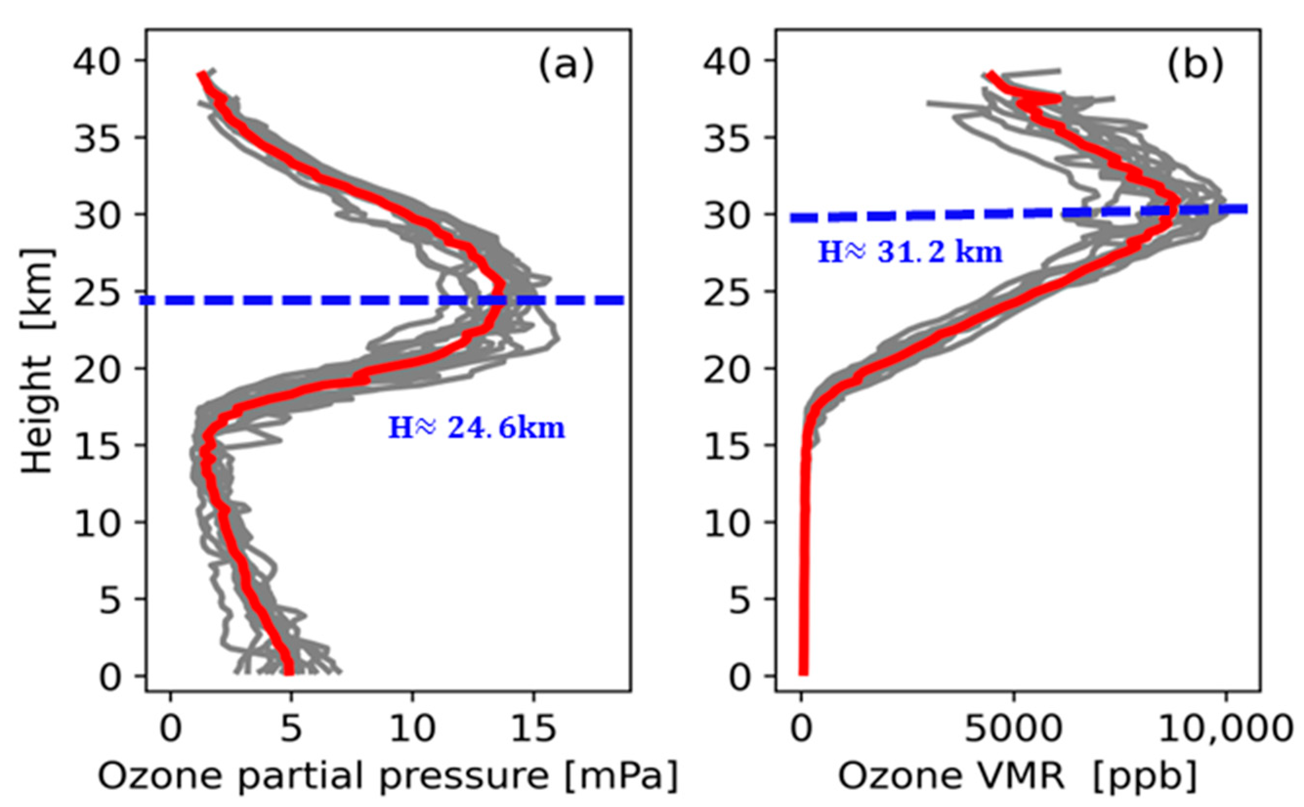
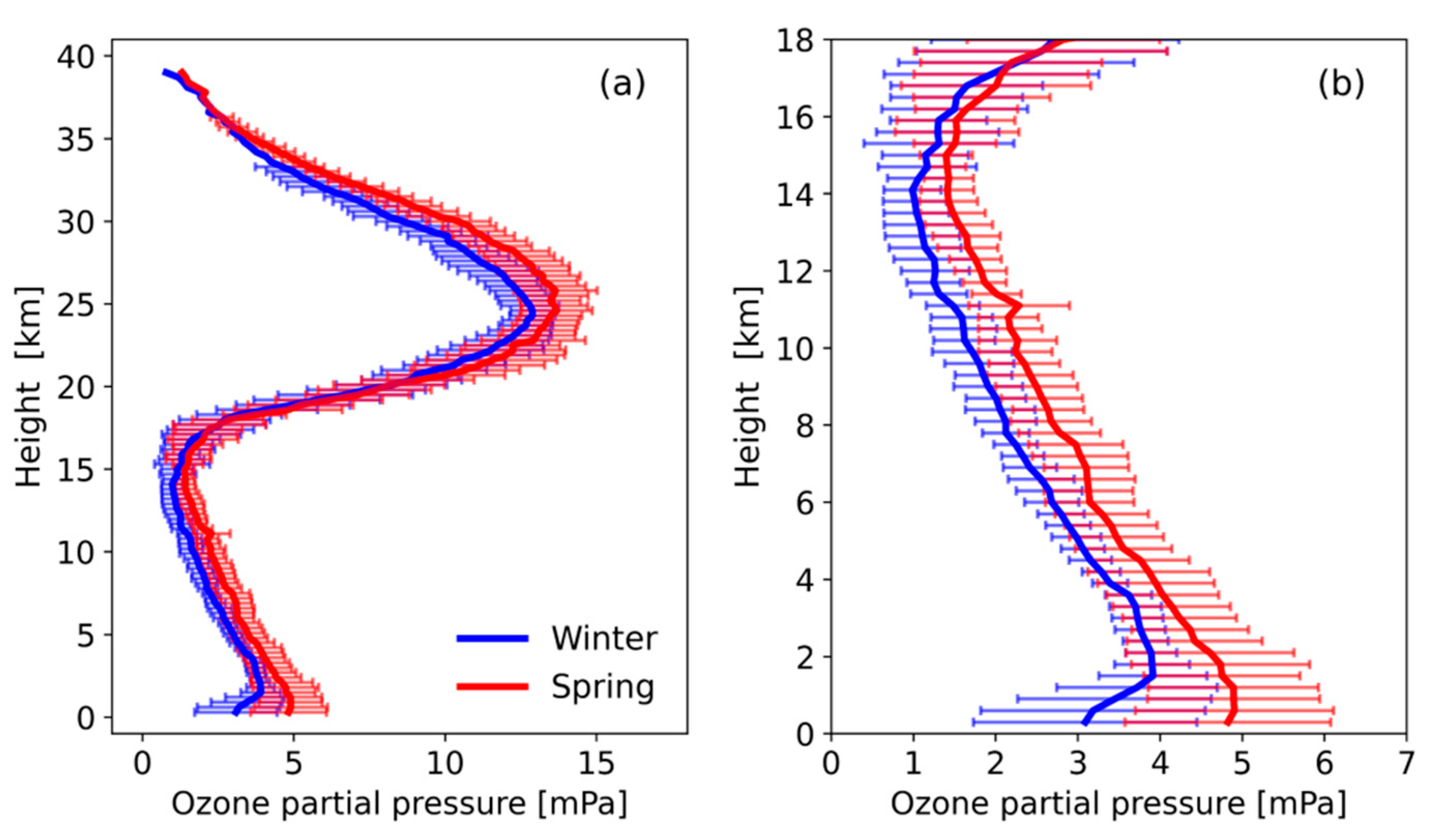
In spring, the maximum height of ozone sounding observations in Shaowu reached 39.6 km, which was 0.9 km higher than that in winter. About 92.3% of the detection heights perfectly covered the upper stratosphere (35–40 km). Ozone partial pressure and OVMR increased compared with winter, and the maximum value increase in the troposphere is 1.6 times;

(2)

In spring, the OVMR in the boundary layer (≤1.5 km) is significantly positively correlated with RH but not with wind speed, which is related to the geographical environment of Shaowu. In the middle and lower troposphere (1.5–12 km), the OVMR has a significant negative correlation with temperature and RH but a significant positive correlation with wind speed;

(3)

The average value of TOC is 496.3 DU in spring, with an obvious increase of 64.4% compared with that in winter. The TOC in the stratosphere increased the most significantly, with an increase of 69.1%. It is an active area of ozone change. Compared with winter, the TOC in the boundary layer increased by 37.2% in spring, and the TOC in the troposphere increased by 23.8% in spring;

(4)

The spring sub-peak phenomenon is different from the winter; the frequency of occurrence increased, reaching 38.5%, followed by the phenomenon of multiple peaks and boundary layer peaks. The peak value of sub-peak VMR is 1.1–1.2 times the average state at the same height, which is reduced compared with winter, but the abnormal value is significantly increased. The RH at some secondary peaks is large than 10%, and the pairing of the sub-peak and its inversion phenomenon increases. In winter, there is a consistent strong westerly flow control at the sub-peak. In spring, some sub-peaks have disordered wind direction and weak wind speed, and some appear after the outbreak of subtropical westerly jets and the rapid increase of wind speed;

(5)

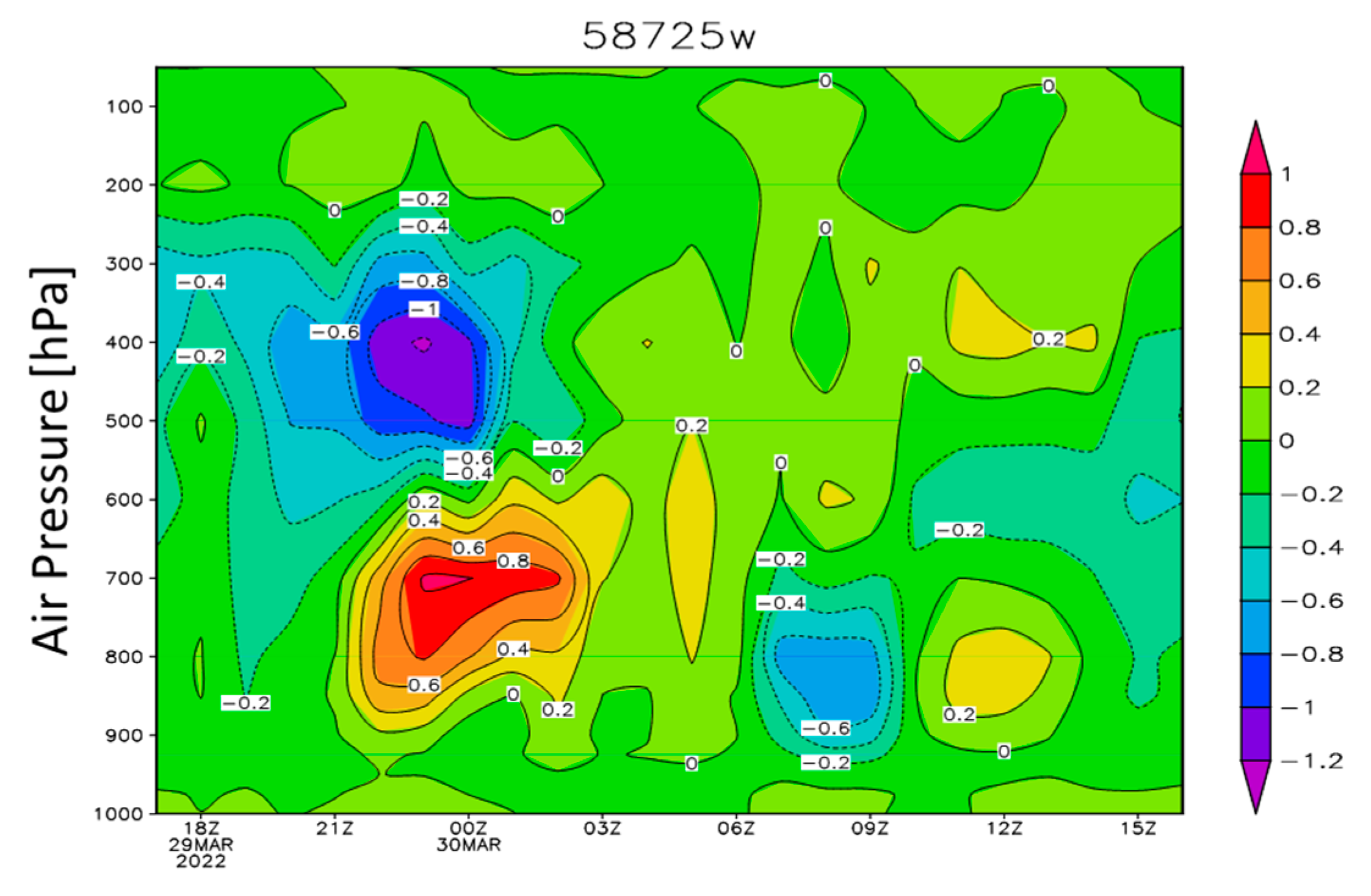
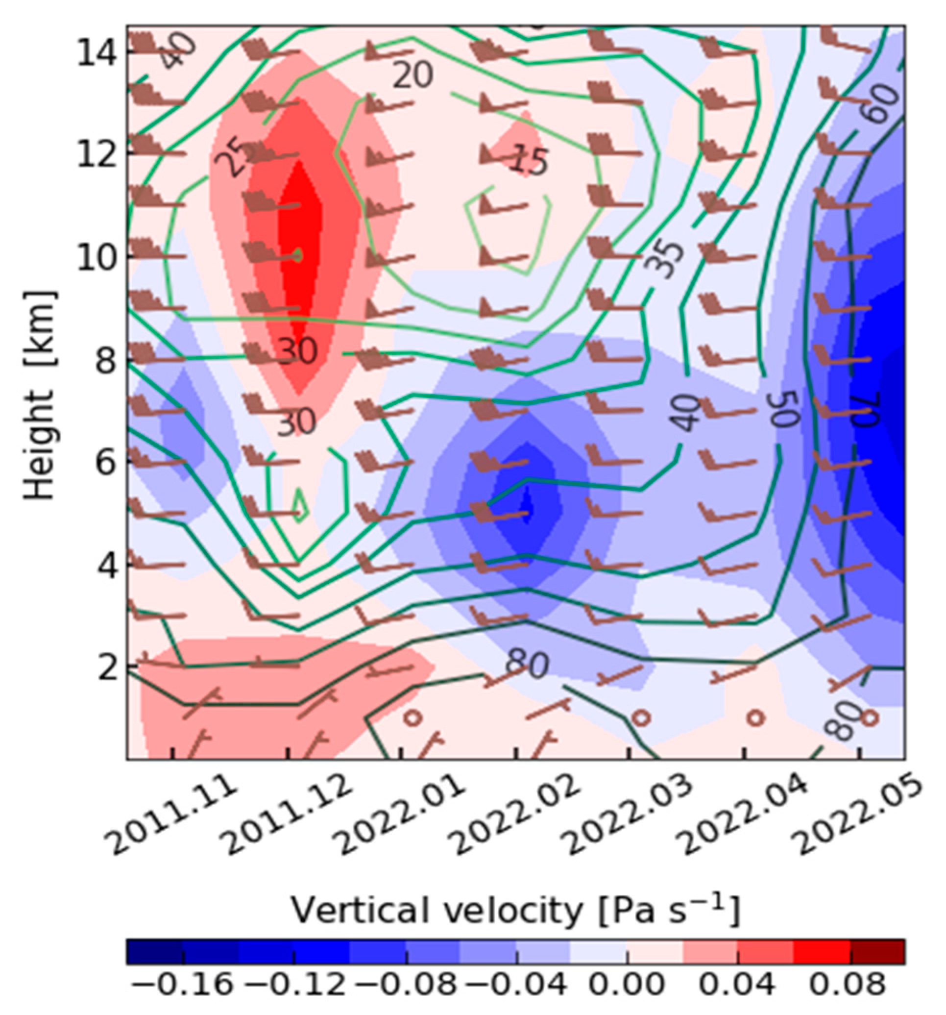
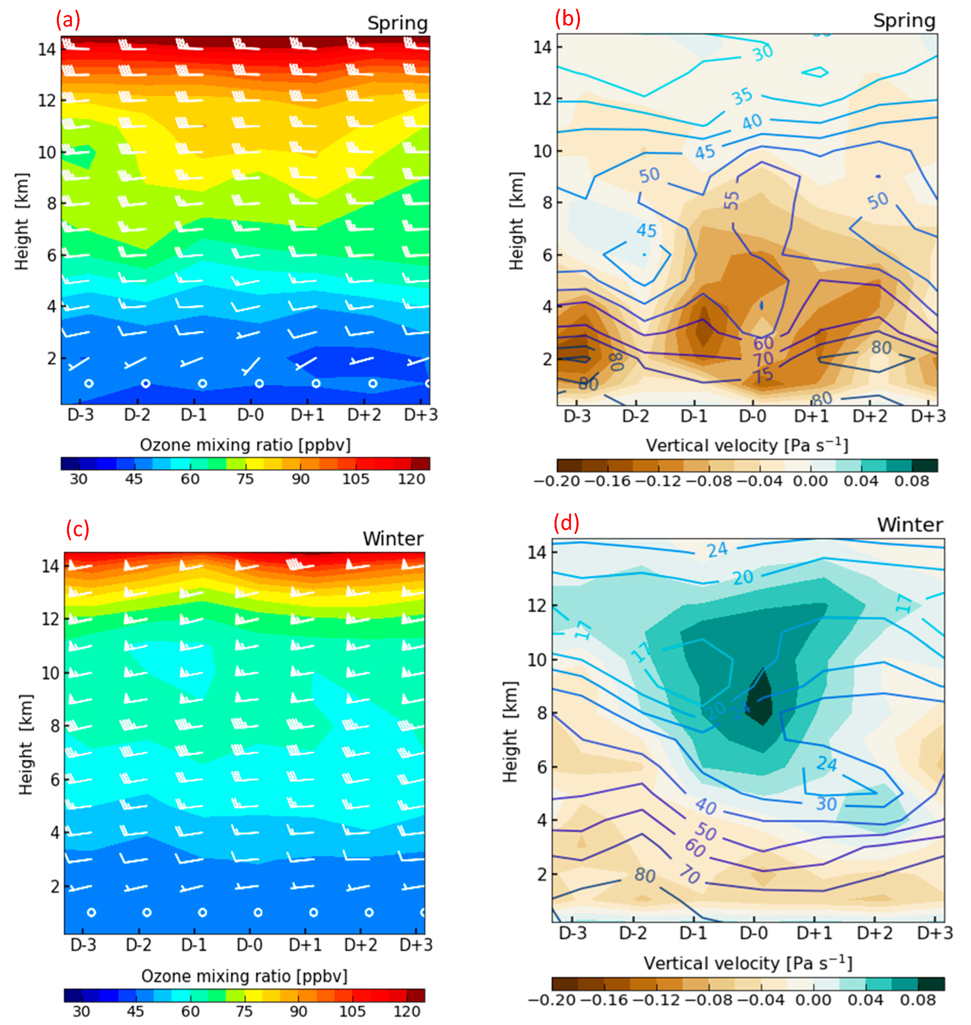
The tropospheric OVMR in spring is significantly higher than that in winter. The near-surface layer is dominated by southwest airflow. The southerly wind on the ozone observation day is stronger; the updraft at the top of the boundary layer is stronger, and the RH is lower than that on the non-observation day. In the middle and upper troposphere (>7 km), the OVMR is distributed in a “funnel” distribution, that is, the OVMR on the ozone observation day and the two days before and after it is higher than that on other days.

References

1. Gaudel, A.; Cooper, R.; Ancellet, G.; Barret, B.; Boynard, A.; Burrows, J.; Clerbaux, C.; Coheur, P.-F.; Cuesta, J.; Cuevas, E.; et al. Tropospheric Ozone Assessment Report: Present-day distribution and trends of tropospheric ozone relevant to climate and global atmospheric chemistry model evaluation. Elem. Sci. Anthr. 2018, 6, 39. [Google Scholar] [CrossRef]
2. Intergovernmental Panel on Climate Change (Ed.) Anthropogenic and Natural Radiative Forcing. In Climate Change 2013—The Physical Science Basis: Working Group I Contribution to the Fifth Assessment Report of the Intergovernmental Panel on Climate Change; Cambridge University Press: Cambridge, UK, 2014; pp. 659–740. ISBN 9781107057999. [Google Scholar]
3. Lefohn, A.S.; Malley, C.S.; Smith, L.; Wells, B.; Hazucha, M.; Simon, H.; Naik, V.; Mills, G.; Schultz, M.G.; Paoletti, E.; et al. Tropospheric Ozone Assessment Report: Global Ozone Metrics for Climate Change, Human Health, and Crop/Ecosystem Research. Elem. Sci. Anthr. 2018, 6, 27. [Google Scholar] [CrossRef] [PubMed]
4. Fleming, Z.L.; Doherty, R.M.; von Schneidemesser, E.; Malley, C.S.; Cooper, O.R.; Pinto, J.P.; Colette, A.; Xu, X.; Simpson, D.; Schultz, M.G.; et al. Tropospheric Ozone Assessment Report: Present-Day Ozone Distribution and Trends Relevant to Human Health. Elem. Sci. Anthr. 2018, 6, 12. [Google Scholar] [CrossRef]
5. Maji, K.J.; Ye, W.-F.; Arora, M.; Nagendra, S.M.S. Ozone Pollution in Chinese Cities: Assessment of Seasonal Variation, Health Effects and Economic Burden. Environ. Pollut. 2019, 247, 792–801. [Google Scholar] [CrossRef]
6. Feng, Z.; Sun, J.; Wan, W.; Hu, E.; Calatayud, V. Evidence of Widespread Ozone-Induced Visible Injury on Plants in Beijing, China. Environ. Pollut. 2014, 193, 296–301. [Google Scholar] [CrossRef]
7. Reich, P.B.; Amundson, R.G. Ambient Levels of Ozone Reduce Net Photosynthesis in Tree and Crop Species. Science 1985, 230, 566–570. [Google Scholar] [CrossRef]
8. White, M.C.; Etzel, R.A.; Wilcox, W.D.; Lloyd, C. Exacerbations of Childhood Asthma and Ozone Pollution in Atlanta. Environ. Res. 1994, 65, 56–68. [Google Scholar] [CrossRef]
9. Wang, T.; Xue, L.; Brimblecombe, P.; Lam, Y.F.; Li, L.; Zhang, L. Ozone Pollution in China: A Review of Concentrations, Meteorological Influences, Chemical Precursors, and Effects. Sci. Total Environ. 2017, 575, 1582–1596. [Google Scholar] [CrossRef]
10. Fioletov, V.E.; Bodeker, G.E.; Miller, A.J.; McPeters, R.D.; Stolarski, R. Global and Zonal Total Ozone Variations Estimated from Ground-Based and Satellite Measurements: 1964–2000. J. Geophys. Res. Atmos. 2002, 107, ACH-21. [Google Scholar] [CrossRef]
11. Harris, N.R.P.; Hassler, B.; Tummon, F.; Bodeker, G.E.; Hubert, D.; Petropavlovskikh, I.; Steinbrecht, W.; Anderson, J.; Bhartia, P.K.; Boone, C.D.; et al. Past Changes in the Vertical Distribution of Ozone—Part 3: Analysis and Interpretation of Trends. Atmos. Chem. Phys. 2015, 15, 9965–9982. [Google Scholar] [CrossRef] [Green Version]
12. Tarasick, D.W.; Fioletov, V.E.; Wardle, D.I.; Kerr, J.B.; Davies, J. Changes in the Vertical Distribution of Ozone over Canada from Ozonesondes: 1980–2001. J. Geophys. Res. D Atmos. 2005, 110, 1–19. [Google Scholar] [CrossRef]
13. Zhang, Z.; Zhang, X.; Gong, D.; Quan, W.; Zhao, X.; Ma, Z.; Kim, S.-J. Evolution of Surface O3 and PM2.5 Concentrations and Their Relationships with Meteorological Conditions over the Last Decade in Beijing. Atmos. Environ. 2015, 108, 67–75. [Google Scholar] [CrossRef]
14. Liu, Y.; Wang, T. Worsening Urban Ozone Pollution in China from 2013 to 2017—Part 1: The Complex and Varying Roles of Meteorology. Atmos. Chem. Phys. 2020, 20, 6305–6321. [Google Scholar] [CrossRef]
15. van Malderen, R.; de Muer, D.; de Backer, H.; Poyraz, D.; Verstraeten, W.W.; de Bock, V.; Delcloo, A.W.; Mangold, A.; Laffineur, Q.; Allaart, M.; et al. Fifty Years of Balloon-Borne Ozone Profile Measurements at Uccle, Belgium: A Short History, the Scientific Relevance, and the Achievements in Understanding the Vertical Ozone Distribution. Atmos. Chem. Phys. 2021, 21, 12385–12411. [Google Scholar] [CrossRef]
16. Chen, Z.; Zhuang, Y.; Xie, X.; Chen, D.; Cheng, N.; Yang, L.; Li, R. Understanding Long-Term Variations of Meteorological Influences on Ground Ozone Concentrations in Beijing During 2006–2016. Environ. Pollut. 2019, 245, 29–37. [Google Scholar] [CrossRef] [PubMed]
17. Chen, X.; Zhong, B.; Huang, F.; Wang, X.; Sarkar, S.; Jia, S.; Deng, X.; Chen, D.; Shao, M. The Role of Natural Factors in Constraining Long-Term Tropospheric Ozone Trends over Southern China. Atmos. Environ. 2020, 220, 117060. [Google Scholar] [CrossRef]
18. Gao, W.; Tie, X.; Xu, J.; Huang, R.; Mao, X.; Zhou, G.; Chang, L. Long-Term Trend of O3 in a Mega City (Shanghai), China: Characteristics, Causes, and Interactions with Precursors. Sci. Total Environ. 2017, 603–604, 425–433. [Google Scholar] [CrossRef]
19. Lal, S.; Naja, M.; Subbaraya, B.H. Seasonal Variations in Surface Ozone and Its Precursors over an Urban Site in India. Atmos. Environ. 2000, 34, 2713–2724. [Google Scholar] [CrossRef]
20. Steinbrecht, W.; Hassler, B.; Claude, H.; Winkler, P.; Stolarski, R.S. Global Distribution of Total Ozone and Lower Stratospheric Temperature Variations. Atmos. Chem. Phys. 2003, 3, 1421–1438. [Google Scholar] [CrossRef]
21. Pu, X.; Wang, T.J.; Huang, X.; Melas, D.; Zanis, P.; Papanastasiou, D.K.; Poupkou, A. Enhanced Surface Ozone during the Heat Wave of 2013 in Yangtze River Delta Region, China. Sci. Total Environ. 2017, 603–604, 807–816. [Google Scholar] [CrossRef]
22. Massagué, J.; Carnerero, C.; Escudero, M.; Baldasano, J.M.; Alastuey, A.; Querol, X. 2005–2017 Ozone Trends and Potential Benefits of Local Measures as deduced from Air Quality Measurements in the North of the Barcelona Metropolitan Area. Atmos. Chem. Phys. 2019, 19, 7445–7465. [Google Scholar] [CrossRef]
23. Jiang, Y.C.; Zhao, T.L.; Liu, J.; Xu, X.D.; Tan, C.H.; Cheng, X.H.; Bi, X.Y.; Gan, J.B.; You, J.F.; Zhao, S.Z. Why Does Surface Ozone Peak before a Typhoon Landing in Southeast China? Atmos. Chem. Phys. 2015, 15, 13331–13338. [Google Scholar] [CrossRef]
24. Zhao, K.; Hu, C.; Yuan, Z.; Xu, D.; Zhang, S.; Luo, H.; Wang, J.; Jiang, R. A Modeling Study of the Impact of Stratospheric Intrusion on Ozone Enhancement in the Lower Troposphere over the Hong Kong Regions, China. Atmos. Res. 2021, 247, 105158. [Google Scholar] [CrossRef]
25. Gallardo, L.; HenríQuez, A.; Thompson, A.M.; Rondanelli, R.; Carrasco, J.; Orfanoz-Cheuquelaf, A.; Velásquez, P. The First Twenty Years (1994–2014) of Ozone Soundings from Rapa Nui (27° S, 109° W, 51 m a.s.l.). Tellus Ser. B Chem. Phys. Meteorol. 2016, 68, 29484. [Google Scholar] [CrossRef]
26. Zheng, Y.; Deng, H.; You, H.; Qiu, Y.; Zhu, T.; Cheng, X.; Wang, H. A Study of the Vertical Distribution and Sub-Peaks of Ozone below 12 Km over Wuyishan Region Based on Ozone Sounding in Winter. Atmosphere 2022, 13, 979. [Google Scholar] [CrossRef]
27. Yan, X.; Zheng, X.; Zhou, X.; Vömel, H.; Song, J.; Li, W.; Ma, Y.; Zhang, Y. Validation of Aura Microwave Limb Sounder Water Vapor and Ozone Profiles over the Tibetan Plateau and Its Adjacent Region during Boreal Summer. Sci. China Earth Sci. 2015, 58, 589–603. [Google Scholar] [CrossRef]
28. Liao, Z.; Ling, Z.; Gao, M.; Sun, J.; Zhao, W.; Ma, P.; Quan, J.; Fan, S.; Liao, Z.; Ling, Z.; et al. Tropospheric Ozone Variability over Hong Kong Based on Recent 20 Years (2000–2019) Ozonesonde Observation. J. Geophys. Res. Atmos. 2021, 126, e2020JD033054. [Google Scholar] [CrossRef]
29. He, Y.; Wang, H.; Wang, H.; Xu, X.; Li, Y.; Fan, S. Meteorology and Topographic Influences on Nocturnal Ozone Increase during the Summertime over Shaoguan, China. Atmos. Environ. 2021, 256, 118459. [Google Scholar] [CrossRef]
30. Li, D.; Bian, J.C.; Fan, Q.J. A Deep Stratospheric Intrusion Associated with an Intense Cut-off Low Event over East Asia. Sci. China Earth Sci. 2015, 58, 116–128. [Google Scholar] [CrossRef]
31. Wang, H.; Chai, S.; Tang, X.; Zhou, B.; Bian, J.; Vömel, H.; Yu, K.; Wang, W. Verification of Satellite Ozone/Temperature Profile Products and Ozone Effective Height/Temperature over Kunming, China. Sci. Total Environ. 2019, 661, 35–47. [Google Scholar] [CrossRef]
32. Hersbach, H.; Bell, B.; Berrisford, P.; Hirahara, S.; Horányi, A.; Muñoz-Sabater, J.; Nicolas, J.; Peubey, C.; Radu, R.; Schepers, D.; et al. The ERA5 Global Reanalysis. Q. J. R. Meteorol. Soc. 2020, 146, 1999–2049. [Google Scholar] [CrossRef]
33. Mao, J.; Wang, L.; Lu, C.; Liu, J.; Li, M.; Tang, G.; Ji, D.; Zhang, N.; Wang, Y. Meteorological Mechanism for a Large-Scale Persistent Severe Ozone Pollution Event over Eastern China in 2017. J. Environ. Sci. 2020, 92, 187–199. [Google Scholar] [CrossRef] [PubMed]
34. Fan, S.; Wang, B.; Tesche, M.; Engelmann, R.; Althausen, A.; Liu, J.; Zhu, W.; Fan, Q.; Li, M.; Ta, N.; et al. Meteorological Conditions and Structures of Atmospheric Boundary Layer in October 2004 over Pearl River Delta Area. Atmos. Environ. 2008, 42, 6174–6186. [Google Scholar] [CrossRef]
Figure 1. The geographical location of (a) the six national meteorological observation stations in mainland China (blue triangles) and (b) the Wuyishan and Shaowu stations (red dots).
Atmosphere 13 01505 g001
Figure 2. Major sounding instruments: (a) CTY-1 ozone sounding sensor and (b) Beidou Satellite navigator.
Atmosphere 13 01505 g002
Figure 3. Vertical profiles of (a) ozone partial pressure and (b) OVMR for the average of all observations (red line), individual profiles (grey line) and the height corresponding to the average value (blue dotted line) during spring 2022 at Shaowu station.
Atmosphere 13 01505 g003
Figure 4. Profiles of ozone partial pressure at (a) the entire detection levels and (b) within the troposphere, averaged across the spring (red line) and winter (blue line). The error bars represent the standard deviation of the individual observations.
Atmosphere 13 01505 g004
Figure 5. Same as Figure 4, but for OVMR.
Atmosphere 13 01505 g005
Figure 6. The TOC over the stratosphere (grey bar), the troposphere (yellow bar), and boundary layer (blue bar), as well as the trend line (black line), derived from each ozonesonde observation from November 2021 to May 2022. The vertical blue dash line means to distinguish winter from spring. (The boundary layer: 0–1.5 km; troposphere (including boundary layer): 0—tropopause height (km); stratosphere: tropopause height (km)—balloon burst height (km)).
Atmosphere 13 01505 g006
Figure 7. Profiles of tropospheric OVMR (black line), air temperature (red line), relative humidity (blue line), inversion structure (blue dash circles) and horizontal winds (vectors) measured on (a) 1 December 2021; (b) 15 December 2021; (c) 29 December 2021 and (d) 19 January 2022. The sub-peak of each profile is highlighted in blue background and the corresponding relative humidity is also shown.
Atmosphere 13 01505 g007
Figure 8. Same as Figure 7, but for the spring.
Atmosphere 13 01505 g008
Figure 9. The distribution of vertical velocity (shading, units: Pa∙s−1) and wind divergence (black contours, units: 10−5∙s−1) at the Shaowu station during 29–30 May 2022 as a function of hours (data from ERA-5).
Atmosphere 13 01505 g009
Figure 10. Variations of the monthly mean vertical velocity (shading, units: Pa∙s−1), horizontal wind (vectors, units: m∙s−1), and relative humidity (green contours, units: %) at the Shaowu city as a function of time and height, derived from ERA5 reanalysis (the ERA5 grid data used is located at 117.50° E, 27.25° N).
Atmosphere 13 01505 g010
Figure 11. The evolution of (a) daily OVMR (shading) and horizontal winds (vectors), and (b) vertical velocity (shading) and relative humidity (contours) at different heights during the three days before and after the day of sounding observation in spring, based on ERA5 reanalysis. (c,d) shows the same as (a,b) but for the winter.
Atmosphere 13 01505 g011