Atmospheric CO₂ and CH₄ Fluctuations over the Continent-Sea Interface in the Yenisei River Sector of the Kara Sea

Abstract

Observations of the atmospheric sources and sinks of carbon dioxide (CO₂) and methane (CH₄) in the pan-Arctic domain are extremely scarce, limiting our knowledge of carbon turnover in this climatically sensitive environment and the fate of the enormous carbon reservoirs conserved in the permafrost. Especially critical are the gaps in the high latitudes of Siberia, covered by the vast permafrost underlain tundra, where only several atmospheric monitoring sites are operational. This paper presents the first two years (September 2018–January 2021) of accurate continuous observations of atmospheric CO₂ and CH₄ dry mole fractions at the recently deployed tower-based measurement station “DIAMIS” (73.5068° N, 80.5198° E) located on the southwestern coast of the Taimyr Peninsula, Siberia, at the Gulf of the Yenisei River that opens to the Kara Sea (Arctic Ocean). In this paper, we summarized the scientific rationale of the site, examined the seasonal footprint of the station with an analysis of terrestrial vegetation and maritime sector contributing to the captured atmospheric signal, and illustrated temporal patterns of CO₂ and CH₄ for the daytime mixed atmospheric layer over the continent–sea interface. Along with the temporal variations reflecting a signal caused pan-Arctic and not very much influenced by the local processes, we analyzed the spatiotemporal distribution of the synoptic anomalies representing the atmospheric signatures of regional sources and sinks of CO₂ and CH₄ for the studied high-arctic Siberian domain of ~625 thousand km², with nearly equal capturing the land surface (54%) and the ocean (46%) throughout the year. Both for CO₂ and CH₄, we have observed a sea–continent declining trend, presuming a larger depletion of trace gases in the maritime air masses compared to the continental domain. So far, over the Kara Sea, we have not detected any prominent signals of CH₄ that might have indicated processes of subsea permafrost degradation and occurrence of cold seeps–still mainly observed in the eastern Arctic Seas—The Laptev Sea and the East-Siberian Sea.

1. Introduction

The Arctic is warming faster than the other parts of the Earth, e.g., [1], with observed air temperature growth at more than twice the rate of the Northern Hemisphere [2,3,4]. The continual warming of the surface air temperature in the Arctic has triggered rapid and alternate changes in terrestrial ecosystems, in particular, a decrease in the duration and extent of the snow cover [5], enhanced vegetation productivity, or the so-called “Arctic greening” [1,6,7], and is causing perennially-frozen ground (permafrost) to thaw [8,9,10,11,12,13]. Warmer temperatures, permafrost degradation, and increased microbial decomposition of soil organic matter are expected to promote a release of stored organic carbon from the Earth into the atmosphere as carbon dioxide (CO₂) and methane (CH₄) [12,14,15,16]. However, the term and the magnitude of the expected feedback between observed and projected warming and enhanced emissions of carbonaceous gases into the atmosphere remain uncertain, e.g., [16,17,18]. Besides the terrestrial responses, the decreasing trends of arctic sea ice volume and extent [19,20], observed warming of sea surface temperatures in the Arctic Ocean, e.g., [21], intense episodic warming in the central shelf sea [22], and the increasing influx of warmer Atlantic water into the Arctic Ocean, e.g., [23], illustrate progressing warming that is capable of destabilizing Arctic subsea permafrost and gas hydrate reservoirs and promoting the further release of methane [24].

Recent efforts to synthesize the terrestrial carbon budget in the Arctic based on sparse eddy covariance (EC) flux measurements have reported contradictory results, e.g., [12]. In general, Arctic tundra ecosystems have been estimated as an annual net sink of carbon dioxide [25], but some sites are now illustrating net CO₂ sources to the atmosphere, e.g., [26,27]. Particular ecosystems may alter in net carbon gain or loss resulting from changes in the physical and biological environment [28], but only the aggregate response across the region throughout the years to decades matters to future climate [29]. Methane has also been paid increased attention given the Arctic is responsible for ~3% [30] of global CH₄ emissions and, along with tropical forests, e.g., [31], presumed to be one of the major hotspots for recent, e.g., [32] and projected CH₄ emissions [33,34] with potential for increase given substantial climate changes [35]. However, the differential response of particular ecosystems and the relatively scarce flux measurements across the Arctic make it challenging to upscale the aggregate effect of terrestrial carbon exchange on the atmosphere, e.g., [12]. Another approach is to measure variations of CO₂ and CH₄ mole fractions in the atmosphere at masts or towers to analyze their emissions and trends, e.g., [36,37,38] by capturing biogeochemical signals and contributions from different sources. Such source differentiation is particularly challenging in the coastal areas where ocean–atmosphere interactions overlapped with the terrestrial biospheric fluxes [39,40]. Measurements at atmospheric towers deal with a large area of influence or “footprint” on scales of hundreds to thousands of square kilometers, e.g., [41]; in contrast, EC towers provide direct flux measurements but represent the local ecosystem-scale domain of a few hectares, e.g., [42] or chamber measurements used for observations on homogeneous ecosystem patches (~1 m²) or individual plant communities [43]. In turn, observations of carbonaceous gases in the atmosphere integrate spatially heterogeneous fluxes but require further interpretation in a model framework to infer surface-atmosphere fluxes since they do not measure them directly. In this respect, inverse modeling of trace gas transport in the atmosphere is a powerful instrument to provide insights into regional to pan-Arctic scale patterns of CO₂ and CH₄, including their seasonal dynamic, interannual fluctuations, and long-term trends.

However, observations of atmospheric CO₂ and CH₄ mole fractions in the pan-Arctic domain are extremely sparse, restricting the spatiotemporal resolution and the accuracy of modeling tools. The sparse data coverage particularly applies to the high-arctic latitudes of Siberia, covered by the vast tundra underlain by permafrost on the area of ~3 million km², i.e., nearly half of northern high-latitude tundra ecosystems [44]. In contrast to the global relevance of those ecosystems for the terrestrial carbon budget, only a few sites continuously measuring atmospheric CO₂ and CH₄ are operational here (Figure 1a): Tiksi on the Sogo Bay, the Laptev Sea [45], the Cape Baranov ice base observatory on the Bolshevik Island, Severnaya Zemlya (currently, is not operational) [45], Ambarchik at the mouth of the Kolyma River, the coast of the East-Siberian Sea [39] and Belyy Island near the Yamal Peninsula, the Kara Sea (currently, is not operational) [46,47].

Recently started continuous measurements of atmospheric CO₂ and CH₄ fluctuations in the southwestern part of the Taimyr Peninsula, at the Gulf of the Yenisei River, on the coast of the Kara Sea [40], fill a significant gap in the trace gas observation network over the high-arctic regions of Siberia. Due to the general west wind drift across those latitudes, the new site is expected to be primarily sensitive to processes in the arctic landscapes of northwestern Siberia. Hence, besides the expected biogeochemical signals from the Arctic and the Arctic Ocean, the location is particularly receptive to trace gas pollution anomalies from the westerly bordered Ob-Yamal domain: the Yamal and the Gydan Peninsula (Figure 1b) that have been extensively explored in terms of oil and gas production during the last decades, e.g., [48] and further developments in the area.

In this paper, we present the results of the accurate continuous observations of atmospheric CO₂ and CH₄ dry mole fractions for the first two years (September 2018–February 2021) of the new station operation, give the scientific rationale of the site, examine the seasonal footprint of the station with an analysis of vegetation and maritime sector contributing to the captured atmospheric signal, and illustrate temporal patterns of CO₂ and CH₄ for the daytime mixed atmospheric layer over the continent–sea interface in the Yenisei River sector of the Kara Sea (Arctic Ocean). Along with the seasonal variations reflecting a signal that is caused in pan-Arctic region and not very much influenced by the local processes, we analyze the spatiotemporal distribution of the synoptic anomalies of trace gases that indicate the atmospheric signatures of regional sources and sinks of CO₂ and CH₄ for the studied high-arctic Siberian domain.

2. Materials and Methods

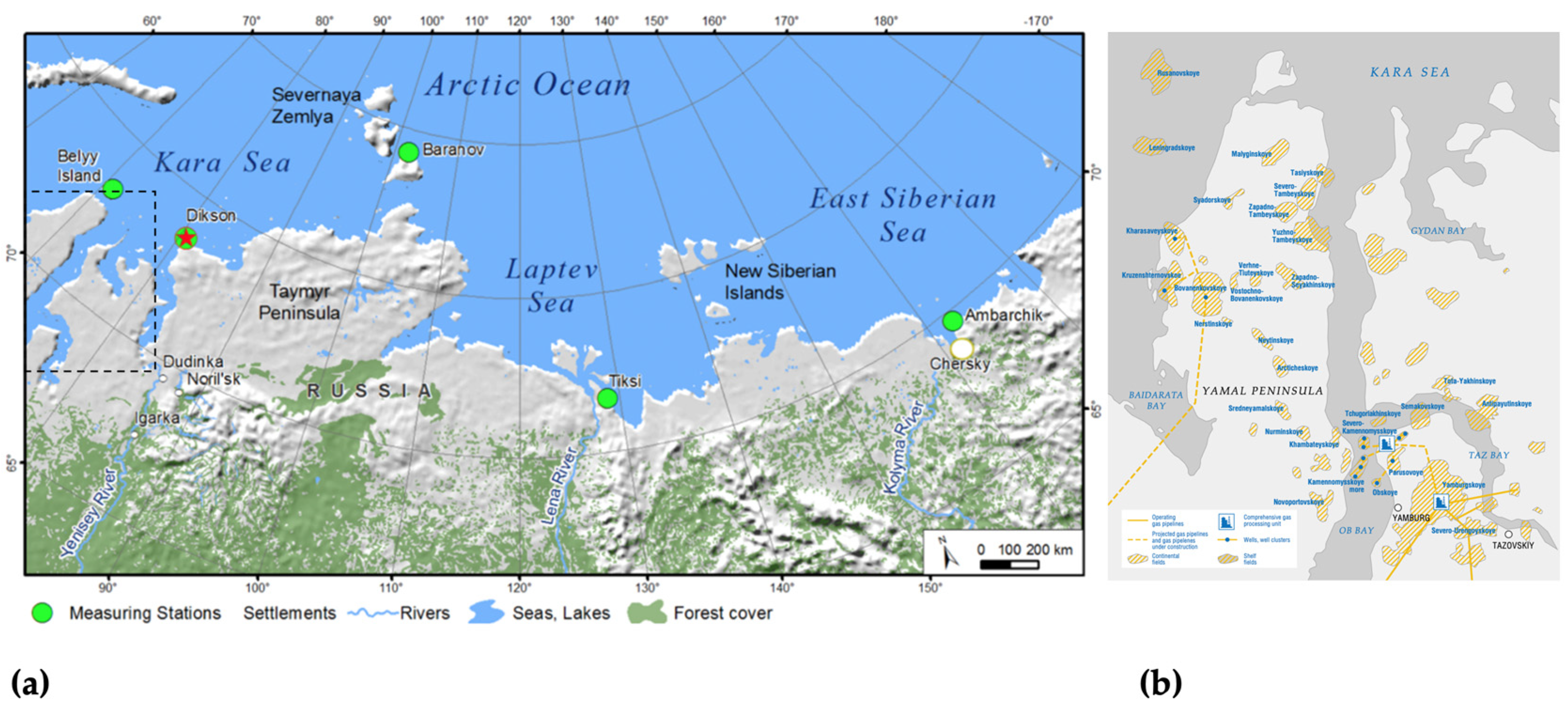
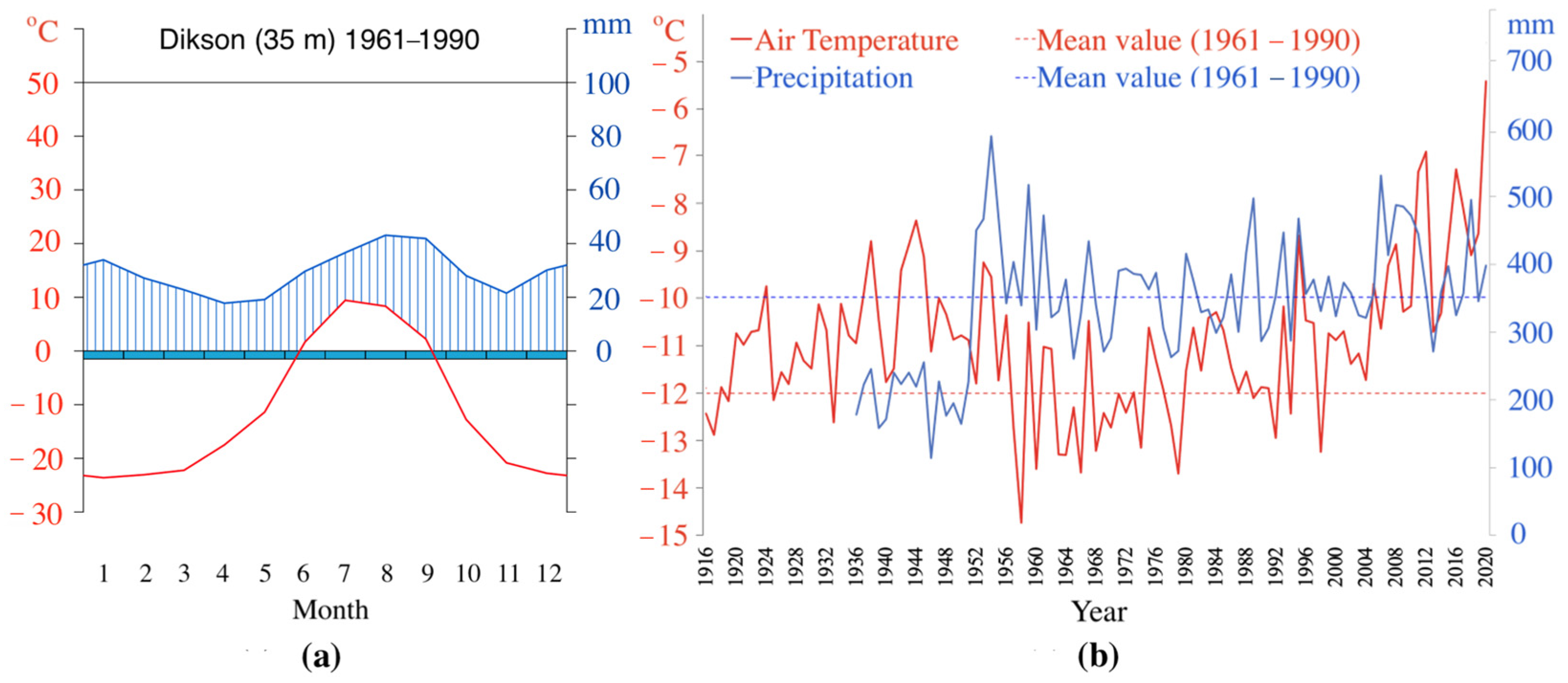
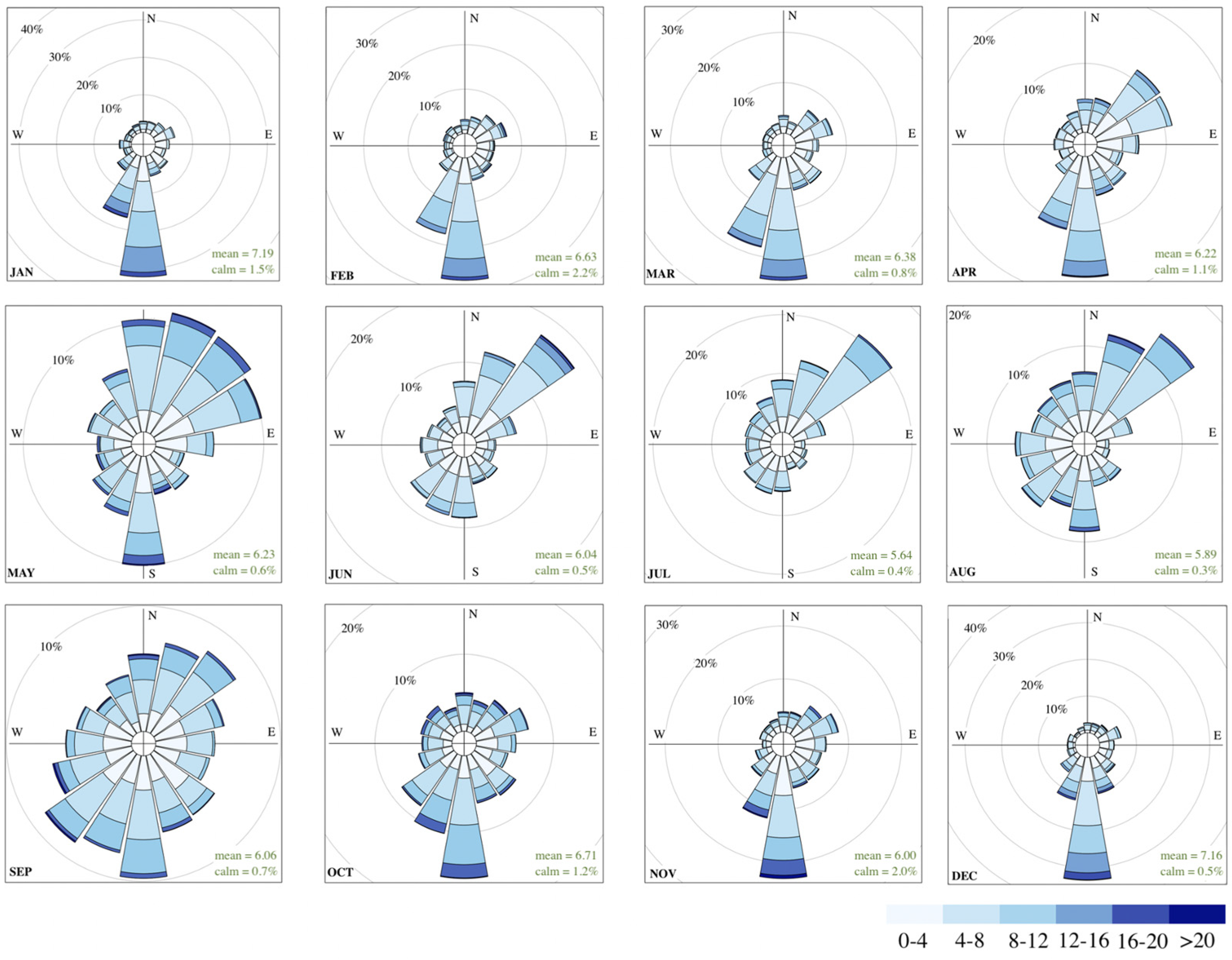
2.1. Study Area

The recently established tower-based measurement station “DIAMIS” (73.5068° N, 80.5198° E) is located on the southwestern coast of the Taimyr Peninsula, a northernmost extension of the Eurasian continent (Figure 1a). Locally, the station is mounted 120 m away from the shoreline of the Gulf of the Yenisei River on the edge of the Dikson–the most northern settlement in Siberia. The Circumpolar Arctic Vegetation Map [49] classifies the study area as the southern part of the arctic tundra that nearly borders with the northern hypoarctic tundra. Further details of the location and description of the surrounding environments can be found elsewhere [40,50].

According to the Köppen climate classification [51], the study area is characterized by a “polar” or “tundra” climate, while a marine influence may be observed on the shoreline where the instrumentation has been deployed. Winters are relatively mild, with a mean air temperature as low as −24.2 °C and frequent intense blizzards, while summer is short, with a mean air temperature achieving +3.76 °C. Daily maximum average temperature of the hottest month and daily minimum average temperature of the coldest month are +21.1 °C and −44.4 °C, correspondingly. Basic meteorological records for the measurement site are given in [40]. Walter and Leith climate diagram [52] for 1961–1990 (Figure 2a) illustrates precipitation and air temperature changes throughout the year for the study area. One can see that the precipitation graph lies above the air temperature indicating wet conditions in the area throughout all seasons.

The mean annual air temperature (MAAT) recorded at the weather station “The Island of Dikson” (WMO ID: 20674), located 3.6 km northwest of the measurement site, for more than 100 yrs. of observations achieves −11.1 °C (Figure 2b). Based on the meteorological archives from the German Climate Data Centre (https://cdc.dwd.de/portal/ (accessed on 6 July 2022)) for WMO ID: 20674, the mean temperature exceeds −12.00 °C in 1961–1990, while achieving −10.14 °C in 1991–2019. Hence, this illustrates an increase of 1.86 °C that is even larger in spring (MAM, +2.66 °C) and winter (DJF, +1.92 °C) but less prominent during summer (JJA, +1.15 °C) and fall (SON, +1.52 °C). Furthermore, in the summer of 2020, the areas adjacent to Dikson demonstrated air temperatures ~5 °C warmer than usual since 1881 [53], which is also reflected in the local meteorological observations at WMO ID: 20674 (Figure 2b). It obviously illustrates the ongoing changes have occurred within the study area that captured the epicenter of the recent Arctic heatwave. However, neither abnormal precipitation amounts observed in 2020 nor long-term trends have been discernible in the whole precipitation record, with a mean rate of 341.3 mm approaching the 1961–1990 mean value of 351.8 mm (Figure 2b).

The multi-year wind distribution for the study area demonstrates a predominance of northeast and southwest wind directions throughout the year (Figure 3). In particular, during colder months (October–March), winds mostly arrive from the south and southwest, with some frequencies of winds blowing from the northeast in spring and from northeast and southeast during autumnal months.

During summer, winds from the north to the northeast are prevailing, while fewer frequencies can be observed from the south to the southwest.

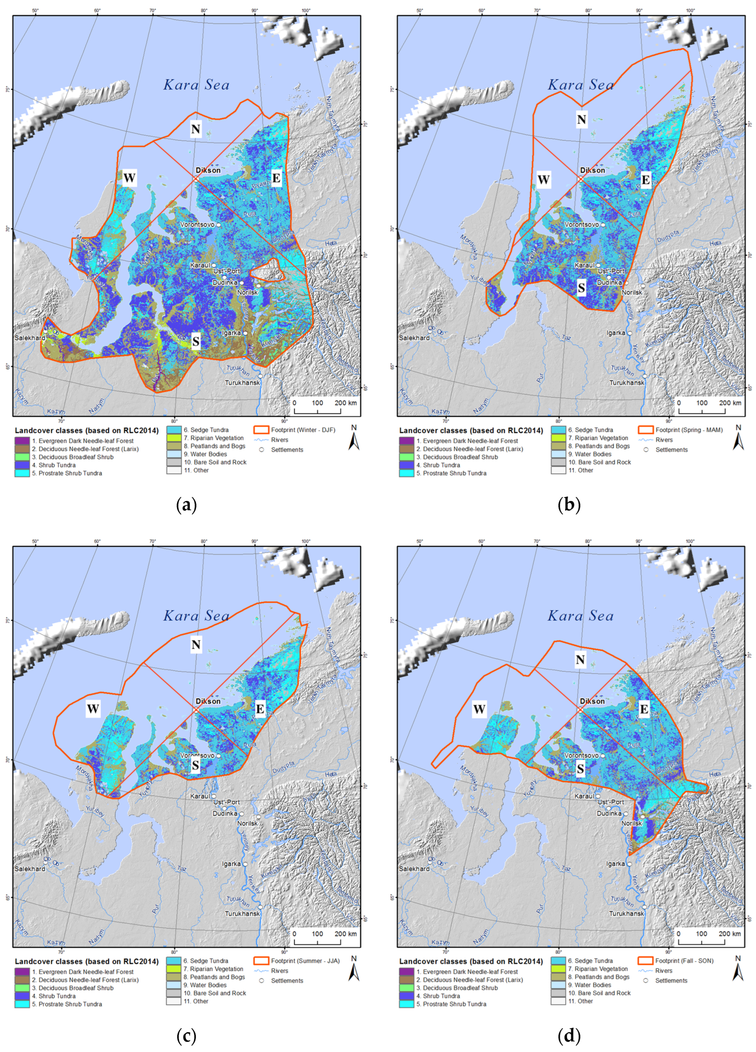
2.2. Seasonal Footprint of the Measurement Site

In order to calculate a “footprint” of the measurement site, we examined the source regions of air parcels moving into the study area, based on the backward trajectory frequency analysis for the measurement period. We computed 5-day backward trajectories of air transport with a daily frequency using the HYbrid Single-Particle Lagrangian Integrated Trajectory model [54] from the ARL NOAA that calculates trajectories based on global wind and meteorology field estimations. The monthly data archives from the NCEP/NCAR Reanalysis Project (Climate Data Assimilation System; CDAS) were utilized as the driving meteorological fields for the computation. After calculations, the 5-day backward trajectories were put on a grid over the computational domain, and the number of trajectory intersections over each grid cell were counted and normalized by the total amount of trajectories. Eventually, we used Terra Norte RLC 2014 map [55] to provide estimates of a vegetation mosaic for the significant domain of influence (>10% frequencies of trajectory intersections observed) in the seasonal footprints.

2.3. Instrumental Setup and Calibrations

The measurement station consists of a metal tower with meteorological sensors and an air inlet installed at the top of the mast at 30 m a.g.l. (35 m a.s.l.). From the tower, a flexible tubing line enters the laboratory room located below, with a cavity ring-down spectroscopy (CRDS) analyzer and the data logger placed inside and mounted into a 19′ measurement rack. The scheme of the instrumental design and technical details of the measurement setup were previously presented elsewhere [40]. Mole fractions of atmospheric CO₂, CH₄, and H₂O are continuously measured by a CRDS analyzer Picarro G2301-f (Picarro Inc., Santa Clara, CA, USA) that passes a regular calibration against pressurized dry air produced at the Max Planck Institute for Biogeochemistry (MPI-BGC; Jena, Germany). In the reference tanks, the greenhouse gas concentrations are traced to the WMO scales: X2007 for CO₂ [56] and X2004A for CH₄ [57]. Since the response of the instrument is linear, three tanks are sufficient for the calibration. A fourth gas tank is utilized as a target for quality control of the calibrations. A calibration cycle automatically starts every 168 hrs. for 25, 20, and 20 min for the High, Middle, and Low tank, correspondingly. Based on these three reference tanks, coefficients for linear calibration have been derived and implemented for the reported time series. The Target tank is probing for 15 min every 24 hrs. The bias for the measured CO₂ (0.03 ppm) and CH₄ (0.03 ppb) in the Target tank for the reported period of observations meets the WMO required range.

Basic meteorological measurements include wind parameters (speed and direction), air temperature, relative humidity, and precipitation. Technical overview of the meteorological instrumentation at the site was earlier given in [40]. The factory-build software of the CRDS analyzer and an external data logger 9210B Xlite (Sutron Corp., Sterling, VA, USA) are utilized for logging time series of trace gas and meteorological variables. Via serial (RS-232) interface, the data logger communicates with the analyzer and collects measured variables with a frequency of 5 s, further producing 1-min averages. The CRDS analyzer obtains a regular time synchronization with an SNTP server, while the 9210B Xlite data logger receives the time of the instrument every 24 h. The measurement system is protected against electrical failures with an uninterruptible power supply APC Smart-UPS X 2200VA SMX2200 (APC Schneider Electric, West Kingston, RI, USA).

2.4. Raw Data Processing

The CRDS analyzer measures CO₂ and CH₄ mole fractions in humid air and includes only a first-order function of water correction [58] that is insufficient, as experimentally confirmed [59]. For the reported study, to calculate the relationship between H₂O and the wet and dry ratios of specific gas in the raw values measured by the instrument, we applied a second-order H₂O correction function, based on the approaches given elsewhere, e.g., [37,60,61].

After water correction and calibration of the raw values, we removed invalid data using a set of filters: for bad analyzer status diagnostics, i.e., Picarro Inc. diagnostic flags were removed manually, flushing the measurement lines prior to and after calibration and the calibration and maintenance operations, and spikes appeared due to contamination from local polluters. Despite the proximity to the settlement, the air probing at the tower is much less prone to local contamination, and wind distribution analysis assures the local position of the mast is beyond or very scarcely receptive to such pollution events. However, there are possible contamination sources in the immediate proximity of the tower: diesel power generator and central boiler of the settlement (~270 m north-northwest (NNW) from the tower). These local polluters might have caused sharp and short-term spikes in CO₂ and, sometimes and depending on the source, CH₄ mole fractions on the timescale of seconds to several minutes. Such signals were detected with an average frequency as low as 3.7% of observations per year, varying from 2% in the winter period and up to 5.4% during summer. We applied the criteria for the spike detection based on [39,62] and adjusted according to the local environment. The raw data passed through strict background filtering and timing, according to [40], which eventually allowed us to identify most of the hourly values of well-mixed air that are represented for the study area and not affected by local polluters.

In order to decompose processed time series into seasonal, trend, and irregular components, we used STL, a seasonal trend decomposition procedure based on loess, a method developed by [63]. Prior to the decomposition procedure, we made an imputation (replacement) of missing values in the time series via the algorithm reported in [64]. During the decomposition procedure with STL, the seasonal component was found by loess smoothing the seasonal sub-series. The seasonal values were removed from the trace gas time series, and the remainder smoothed to find a trend. The overall level was removed from the seasonal component and added to the trend component. This process was repeated several times. Finally, the remainder component represented the residual from the seasonal values plus trend fit. For the subtracted residuals (or anomalies), we calculated the angular distribution along with the prevailing wind directions throughout the seasons and merged the defined anomalies of atmospheric trace gases to four geographical domains in the footprint.

3. Results and Discussion

3.1. Seasonal Footprint Analysis: Contribution of the Land Surface and the Ocean

The average footprint area reaches ~625 thousand km² (Figure 4), varying among the seasons from ~490 thousand km² during fall up to maximal values of ~900 thousand km² in winter, and implies a nearly equal contribution of the land surface (54%) and the ocean (46%) throughout the year. The seasonal pattern shows a dominant influence of the continent in winter (73%) while achieving the highest rates as of 60% of the oceanic input during the summer months. In general, seasonal footprint applies a presumably pristine air coming from the Kara Sea (Arctic Ocean) in late spring to fall, however, with still biogeochemical signals possible from the continent. Meanwhile, during the frost period, the measurement site is ultimately receptive to the continental part of northwestern Siberia, capturing biogeochemical signals from surrounding ecosystems (e.g., winter CH₄ emissions) [34] and transporting polluted air masses from the Ob-Yamal domain (Yamal and Gydan Peninsula), a subject of extensive exploration in terms of oil and gas production as shown in (Figure 1b) and reviewed by [48]. As to the land surface, in general, the vegetation mosaic of the footprint throughout the seasons demonstrates the predominant contribution of sedge tundra ecosystems (21%), shrub tundra (18%), and wetlands (12%) (

Table 1. Land cover classes in the footprint throughout the seasons based on Terra Norte RLC 2014 vegetation map [55].

No.	Land Cover Classes	Area, km2				Area, %
		DJF	MAM	JJA	SON	DJF	MAM	JJA	SON
1	Dark coniferous f.	4701	0	0	0	1	0	0	0
2	Larch forest	39,915	44	0	2799	4	0	0	1
3	Deciduous shrubs	8793	323	6	1485	1	0	0	0
4	Shrub tundra	167,881	76,267	44,302	57,328	18	14	8	12
5	Pr. shrub tundra	53,887	23,642	29,269	22,904	6	4	5	5
6	Sedge tundra	193,103	114,503	94,430	123,553	21	20	17	25
7	Coastal vegetation	9530	424	0	5	1	0	0	0
8	Wetlands	169,810	60,222	41,624	48,684	19	11	8	10
9	Water	244,877	282,005	325,826	224,452	27	50	60	46
10	Bare soil/rocks	18,591	4885	5542	5804	2	1	1	1
11	Other	1740	4	2	158	0	0	0	0
	Total area	912,827	562,319	541,001	487,172	100	100	100	100

). However, during winter, biogeochemical signals might have been traced from the more southernly growing larch forests (4%), dark coniferous forests (1%), and deciduous broadleaf shrubs (1%).

Considering a spatial arrangement of source regions in the footprint throughout the seasons and further differentiation of the atmospheric signals, we have defined four geographical domains based on the corresponding merging ranges of the angular distributions.

The contribution of land cover types (classes) and water areas within the defined domains in the two sectors (continent/ocean) is summarized in

Table 2. Land cover classes (%) in the footprint (Terra Norte RLC 2014) throughout the seasons, arranged to geographical domains and sectors.

		Winter (DJF)				Spring (MAM)				Summer (JJA)				Fall (SON)
		Ocean		Land		Ocean		Land		Ocean		Land		Ocean		Land
No.	Land Cover Classes	N	W	S	E	N	W	S	E	N	W	S	E	N	W	S	E
1	Dark coniferous f.	0	0	1	0	0	0	0	0	0	0	0	0	0	0	0	0
2	Larch forest	0	0	4	0	0	0	0	0	0	0	0	0	0	0	0	0
3	Deciduous shrubs	0	0	1	0	0	0	0	0	0	0	0	0	0	0	0	0
4	Shrub tundra	0	1	14	3	0	0	10	4	0	2	3	4	0	1	5	6
5	Pr. shrub tundra	0	1	3	2	0	0	2	3	0	2	1	3	0	1	1	2
6	Sedge tundra	0	2	12	8	0	0	11	8	0	4	5	8	0	3	9	14
7	Coastal vegetation	0	0	1	0	0	0	0	0	0	0	0	0	0	0	0	0
8	Wetlands	0	1	15	2	0	0	8	2	0	2	3	2	0	1	5	4
9	Water	8	8	9	2	32	8	8	4	27	24	5	4	13	25	5	3
10	Bare soil/rocks	0	0	1	1	0	0	0	0	0	0	0	1	0	0	1	1
11	Other	0	0	0	0	0	0	0	0	0	0	0	0	0	0	0	0
	Total-domains	8	13	61	18	32	8	39	21	27	34	17	22	13	31	26	30
	Total-sectors	21		79		40		60		61		39		44		56

.

The selected domains in the footprint (Figure 4) are as follows: (1) Northern or oceanic domain (N; angular range: NW…NE)–the pristine domain of 116 094 ± 55 684 km², with a mean area in the footprint as of 20.1 ± 11.2%, depending on the season and is expected to be receptive exclusively to the Arctic Ocean (ocean: 98.9 ± 0.1%; land: 1.0 ± 0.1%); (2) Western or mixed domain (W; angular range: NW…SW) of 123 944 ± 59 832 km², with a mean area in the footprint as of 21.4 ± 13%, where both oceanic (76.3 ± 12%) and continental (23.7 ± 12%) influence of the upper extension of the Yamal Peninsula may be detected; (3) Southern or continental and presumably polluted domain (S; angular range: SE…SW) of 248 409 ± 208 712 km² (land: 78.6 ± 7%; ocean: 21.4 ± 7%)–the most extended domain during winter, with a mean area in the footprint as of 35.8 ± 18.5%, which primarily represents the southwestern part of the Taimyr Peninsula and partially receptive to be further hospitable and gas-field-explored territories of the Ob-Yamal area (Figure 1b); (4) Eastern domain (E; angular range: NE…SE) of 137 382 ± 24 116 km², with a mean area in the footprint as of 22.7 ± 4.6%, which may be considered as a relatively pristine continental domain (land: 86.3 ± 4%; ocean: 13.7 ± 4%) that is ultimately influenced by the eastern and inhospitable part of the Taimyr Peninsula, hence representing relatively pristine tundra ecosystems in the study area. Domains 1 and 2 are expected to represent the maritime sector, while 3 and 4 are considered part of the continental sector. In turn, domains 1, 2, and 4 are comparatively pristine, opposite to domain three, which has been assumed to be polluted.

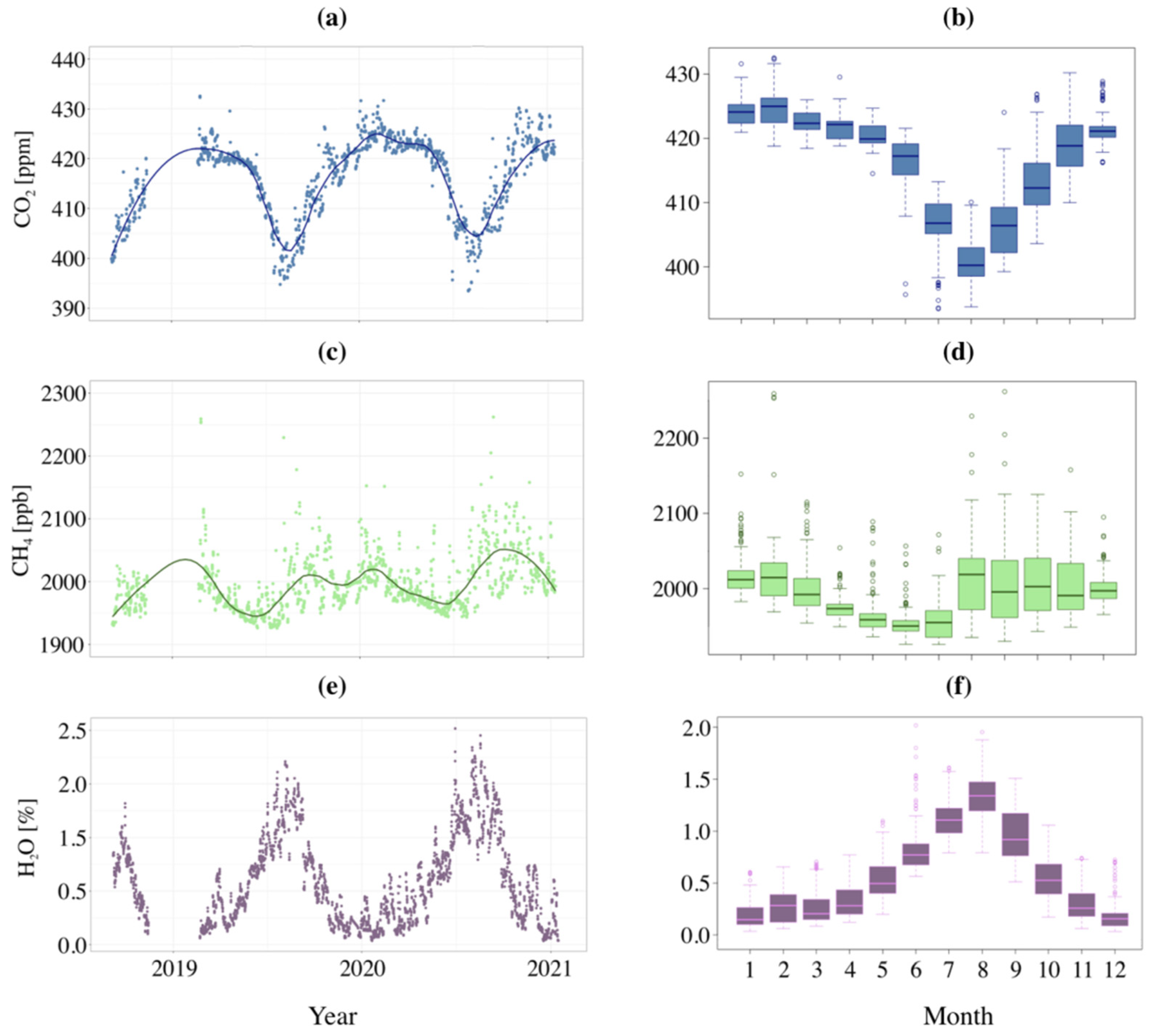
3.2. Temporal Fluctuations of Carbon Dioxide and Methane in the Coastal High-Arctic Atmosphere

As elsewhere [36,39,45,46,47,65,66], the annual dynamic of atmospheric CO₂ and CH₄ shows a seasonal pattern (Figure 5a,b), that is, given a coastal high-arctic location of the site, expected to be primarily related to local environments and proximity to the Arctic Ocean (AO). The detailed overview of the seasonality for CO₂ and CH₄ in the study area was reported earlier [40], while herein we give a longer-term record, focusing more on links of the observed trace gas fluctuations with the footprint of the measurement site and clarifying the contribution of the AO to the atmospheric signals.

Briefly, the seasonal pattern of CO₂ shows a sharp decline and eventual minimum during summer months (August: 400.7 ppm) and reaches a maximum in winter (February: 424.9 ppm), while a particular second peak might have occurred by late winter along with ice melting and the appearance of ice-free areas in the ocean, promoting an immediate release of CO₂ stored beneath the ice into the atmosphere [67,68,69]. However, our winter observations are predominantly receptive to continental air (up to 77% of events) that might have interfered with expected CO₂ signals from the AO. Winter footprint that is the most extended into the continental part during frost period (Figure 4a) illustrates the dominant contribution of the land surface (Table 2) in atmospheric CO₂ fluctuations. Later, possible enhancements of CO₂ that might have been expected until late spring along with the massive ice break-up events could be compensated by a biogenic uptake of carbon dioxide. Since spring, the input of the AO in the footprint becomes more pronounced as well (Figure 4b,c and Table 2); however, the CO₂ declining trend along with winds still mostly blowing from the continent (63%) (Figure 3) may demonstrate a global trend: a startup of CO₂ uptake by terrestrial vegetation in the more southern regions (since March) and local early photosynthesis, which was documented in the AO, e.g., [67,68], while the land surface in the spring footprint of the station (Figure 4b and Table 2) is presumed to be still dormant until June.

Unlike to frost period, in summer (Figure 4c and Table 2), we have observed that an increased influence (up to 62% of the observations) of the air masses occurred over the AO, mostly travelling from the north to northeast (38%) and northwest (24%) (Figure 3), that might have significantly contributed to atmospheric CO₂ levels with a transport of comparatively pristine air masses. To confirm this suggestion, we have applied simultaneous observations of atmospheric carbon dioxide and methane mole fractions during early fall of 2020 over the Kara Sea domain (75–85° E) in the “DIAMIS” footprint (Figure 4), made at 15 m a.s.l. with a CRDS analyzer Picarro G2301 (Picarro Inc., USA) installed on board of the research vessel “Academician Mstislav Keldysh” (Arctic campaign AMK-85) (Figure 6a), and in the coastal atmosphere at the measurement station (Figure 6b). Given the higher absolute values of atmospheric CO₂ in fall, oceanic observations have illustrated noticeably lower maritime CO₂ atmospheric values (406 ± 1.42 ppm) compared to the corresponding coastal averages (411.3 ± 1.33 ppm). Furthermore, observations of CO₂ mole fractions over the Kara Sea have demonstrated a declining trend from the west (408.4 ppm) to the east (403.9 ppm) (Figure 6a) in the oceanic part of the footprint (Figure 4d). A similar decreasing trend was also noted by B. Belan with colleagues [70] by the results of aircraft observations over the AO. Based on their findings [70], the Kara Sea was considered relatively pristine in respect to atmospheric CO₂ with ~5 ppm fewer rates compared to the other Arctic Seas. Meanwhile, continental contribution in our summer observations had not exceeded 38% from the south (25%) to southeast (13%) (Figure 3), reflecting local signals both by biotic and anthropogenic origin from the southwestern part of the Taimyr Peninsula and further continental areas of Siberia (Figure 4c).

Given the summer CO₂ values observed at the “DIAMIS” station, the seasonal amplitude of CO₂, a difference between summer minimum (uptake) and winter maximum (release), achieves ~22 ppm, which is slightly higher than the values reported for Ambarchik (20 ppm) [39], Tiksi (22 ppm), and Cape Baranova ice base observatory (19.6 ppm) [45]. CO₂ minimum expectedly shifts to later dates compared to the more southern mid-continental domain as reported for “ZOTTO” observatory in central Siberia by [71], and presumably driven both by a terrestrial uptake of the surrounding ecosystems and a strong contribution of the relatively pristine air masses travelling from the AO (Figure 4c and Table 2).

In contrast to CO₂, amplitude of atmospheric methane demonstrates a flatter baseline that varies less throughout the year (Figure 5c,d), but a seasonal trend with winter maximum (February: 2015.8 ppb) and mid-summer minimum (June–July: ~1950 ppb) is noticeable. During winter months (polar night), photochemical reactions with hydroxyl radicals (OH) do not occur, e.g., [72], as destruction of CH₄ is considered a primary factor determining the seasonal cycle in the more southern regions (30–60° N), e.g., [73], while in higher latitudes, atmospheric transport and seasonally dependent CH₄ sources might have played a more essential role. Since biogenic CH₄ sources during the frost period are primarily dormant, besides some exceptions (e.g., winter CH₄ emissions [34]), abiotic signals might prevail. The spatial distribution of CH₄ signals equally corresponds to a location of the source regions mostly over the continental domain of the winter footprint (Figure 4a) capturing the southwestern part of the Taimyr Peninsula, westerly bordered areas of the Yamal, the Gydan Peninsula and, located further northwest, the Taz Peninsula. Particularly, the Ob-Yamal domain and the Taz Peninsula [40,48] are presumed to be the major source regions (Figure 1b) where we have observed prominent pollution signals to transport downwind to the measurement site in frost period. During the transition time, by spring (MAM) (Figure 4b), given the large portion of CH₄ accumulated beneath the ice during frost period, which is estimated ~3 times longer than the open water time, CH₄ released into the atmosphere during ice break-up is presumed substantial, e.g., [74]. Hence, while biotic methane sources may be still negligible in the area, a part of CH₄ enhancements (Figure 5c,d) observed by late spring (May–June) might have occurred during the massive ice melting events even though a portion of this flux could be slightly attenuated due to oxidation of CH₄ in the water column.

Similar to CO₂, by the late spring and summer, the seasonal pattern of atmospheric CH₄ contains more signals from the Arctic Ocean. The AO area that is captured in the footprint achieves 40% and 60% (Figure 4b,c and Table 2) in spring and summer, respectively. Until recently, terrestrial ecosystems have been considered to contribute to the Arctic CH₄ maximum, while the AO has been presumed to underestimate. For instance, N. Shakhova with colleagues [74] considers a significant part of the AO, particularly the shallow shelf (<50 m), as an atmospheric CH₄ source, which contributes as much as 68% of the total methane release from the continental Arctic north of 60° N as noted by [75]. Our measurements of atmospheric methane made in early fall of 2020 over the Kara Sea domain (75–85° E) in the “DIAMIS” footprint (Figure 4d) at the research vessel “Academician Mstislav Keldysh” (Figure 6a) and at the station (Figure 6b) illustrate essentially lower CH₄ values (1987 ± 3 ppb) over the AO, compared to the corresponding coastal averages (2001.4 ± 5.9 ppb). However, B. Belan with colleagues [70] has reported autumnal values of atmospheric CH₄ recorded over the Kara Sea as of 2055–2090 ppb. Unlike CO₂ levels that have been presumed comparatively pristine above the Kara Sea [70], flight observations of CH₄ have shown atmospheric air being more enriched by methane compared to the other Arctic Seas. Hence, the discrepancy between maritime CH₄ atmospheric rates reported from a flight campaign (2055–2090 ppb [70]) and our research vessel-based values (2001.4 ± 5.9 ppb) of CH₄ for the Kara Sea might achieve as much as ~70–100 ppb.

Along with the oceanic signals that we have recorded, ~38% of summer observations have been influenced by the continent, representing the southern part of the Taimyr Peninsula and the upper extensions of the Yamal and the Gydan Peninsula (Figure 4c). Unlike to frost period [40], we have not observed pollution anomalies from the Ob-Yamal area in summer as footprint cuts the lower parts of the Yamal and the Gydan Peninsula that are mostly industrially developed. However, biogenic continental CH₄ sources might be essential and significantly differ, as reported by [76] for different landscapes in the western part of the Yamal Peninsula. Along with a decline in CH₄ triggered by warming of the seasonally thawed soil layers, we have observed extensive enhancements since early summer (Figure 5c,d), likely related to biogenic sources of CH₄. Unlike the observed CO₂ minimum in August (Figure 5a,b), the warmest month throughout the year, CH₄ minimal rates occur earlier in June (1950.2 ppb) and July (1953.5 ppb). Furthermore, the CH₄ peak that is comparable to winter methane maximum is discernible in August (Figure 5c,d) and promoted by active biogenic emissions in the surrounding ecosystems (Figure 4c and Table 2). Eventually, during fall (SON) (Figure 4d) and further frost period, our observations are predominantly receptive to the continental influence (64–77% of the events), with air masses mostly coming from the south (16–31%) and southwest (10–15%) (Figure 3). While a large part of the active soil layer may stay unfrozen during colder months with temperatures fluctuating around 0 °C (“zero curtain” period [34]), we might have observed sporadic CH₄ enhancements until November [40]. In winter, when atmospheric water vapor levels are low (Figure 5e,f), both CO₂ and CH₄ become more important for the radiation budget.

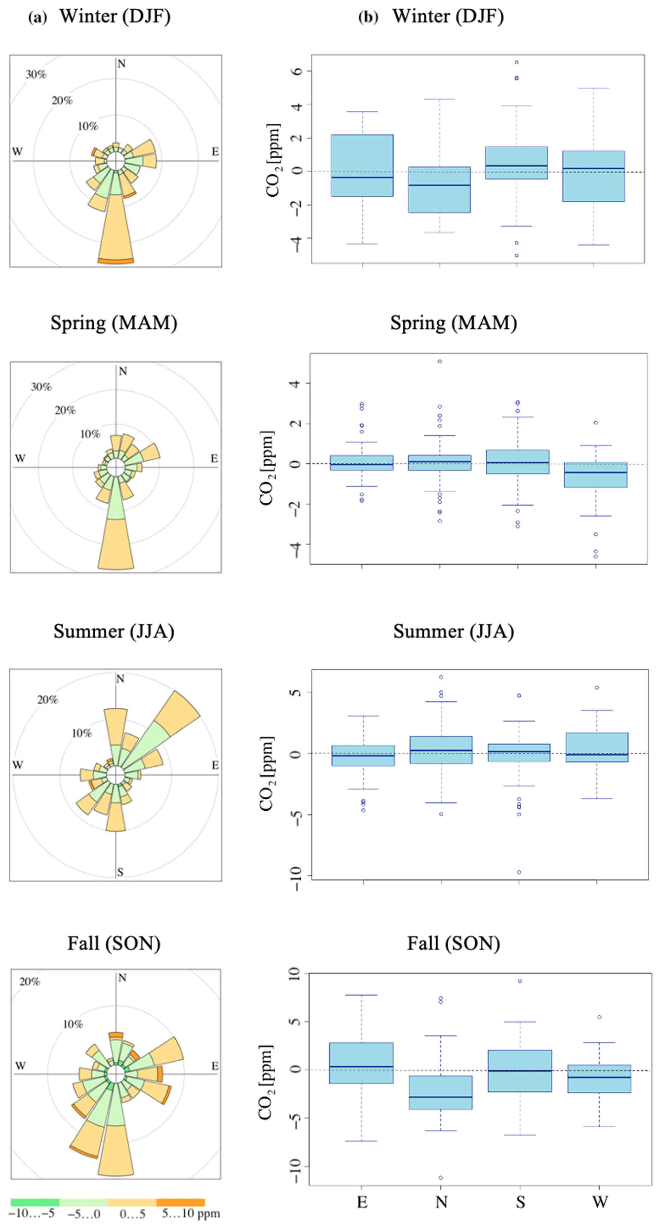
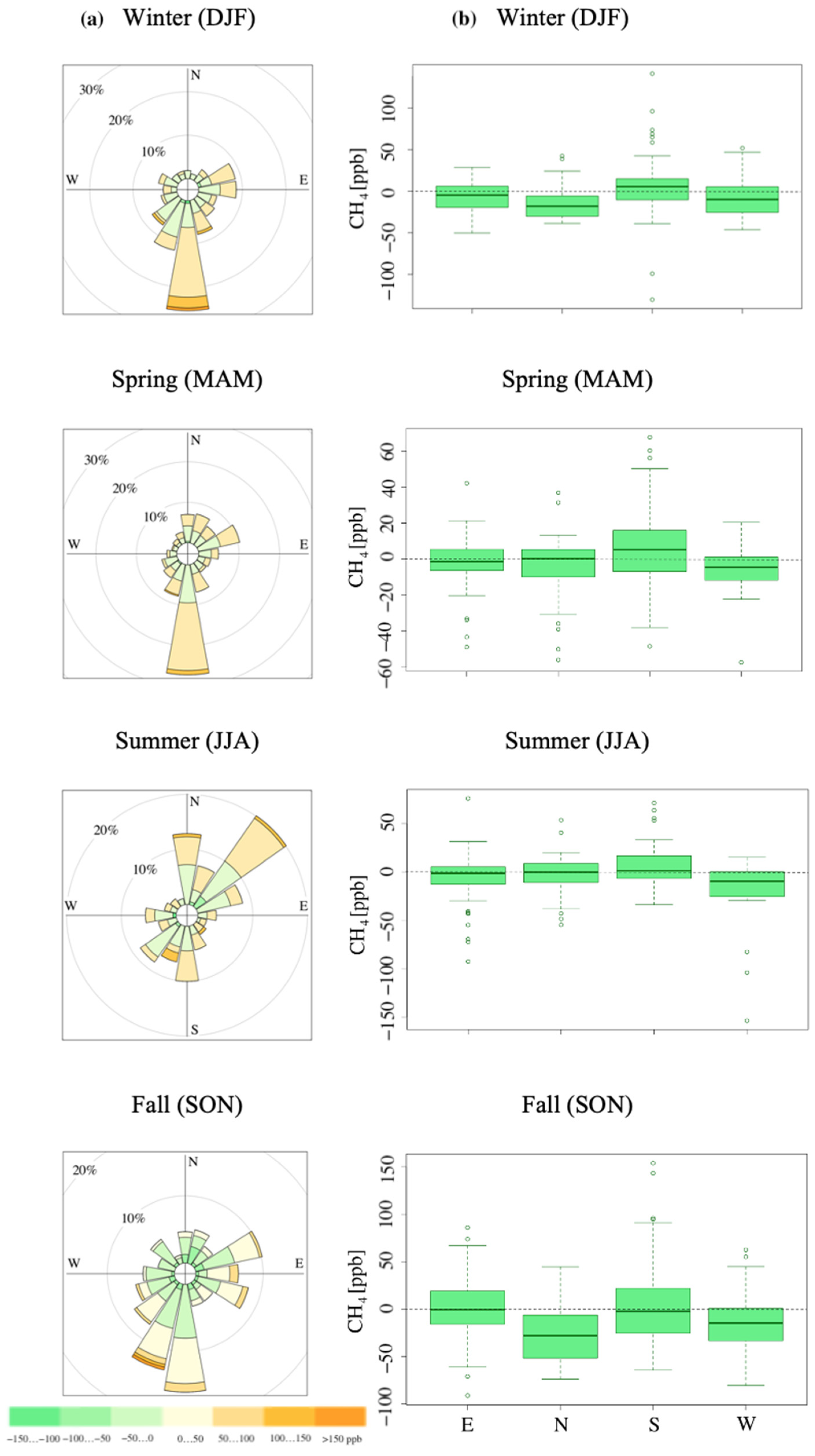
3.3. Spatiotemporal Distribution of CO₂ and CH₄ Anomalies in the Coastal High-Arctic Atmosphere

In contrast to the smooth seasonal cycle of CO₂ and CH₄ shown in Section 3.2 and reflecting a signal that is caused pan-Arctic and not very much influenced by the local processes, the deviations from the seasonal cycle, the synoptic variations or anomalies of a particular gas represent the atmospheric signatures (signals) of regional sources and sinks captured over the surrounding area. The angular distribution of CO₂ signatures along the prevailing wind directions throughout the year is presented in Figure 7a. The most frequent CO₂ signals occurred over the continent in winter (79%) and mostly traveled from the south (25%) and southwest (12%), reflecting a significant role of the southwestern part of the Taimyr Peninsula as a source region for our observations, but also abiotic signals from the gas/oil fields in the Ob-Yamal area (Figure 1b) may be hidden in the observed anomalies as also earlier reported in [40]. In spring, continental influence has slightly decreased (68%), with air masses still primarily coming from the south (27%) (Figure 7a), hence cutting possible pollution anomalies from the west as footprint of the station indicates (Figure 4b).

Summer months have demonstrated greater oceanic (55%) input, while during fall, the distribution dropped back to the continental predominance (68%) of the detected CO₂ anomalies. In general (Figure 7b), the prevailing CO₂ signals that have been observed throughout the year were the average negative anomalies of −0.2 ± 0.3 ppm over the continent (65%), while the ocean (35%) has demonstrated a bit lower negative signature of −0.4 ± 0.7 ppm, assuming a larger depletion of CO₂ in air masses traveled from the AO compared to terrestrial ecosystems. However, due to the relatively high deviations along with the observed anomalies, the reported differences between the two main sectors: ocean–continent (F = 1.12; P = 0.29) and throughout the seasons (F = 1.27; P = 0.29) are not statistically significant, while a combination of both factors (sector–season) shows differences (F = 7.12; P = 0.00039). Notably, a post-hoc Tukey HSD test indicates differences within the oceanic sector for groups: fall vs. spring (P = 0.03268) and fall vs. summer (P = 0.00022), while not significant for the other seasons. Hence, in some extent, we are more confident to discuss about tendencies of a particular domain or season regarding carbon balance, even though considering the absolute average values.

For the statistically differed cases, the negative CO₂ signatures from the AO have been observed in spring (−0.2 ± 0.4 ppm) and values as low as −1.6 ± 1.2 ppm recorded during fall, while in summer, even positive values as of +0.6 ± 1.3 ppm have been found. In particular, within the oceanic sector (Figure 7b), the most pronounced signals during fall have occurred along with pristine air masses coming from the northern domain and depleted by CO₂ (−2.0 ± 1.3 ppm) while showing the less prominent values (−0.6 ± 0.8 ppm) for western (mixed) domain due to a proposed overlap with a continental part and capturing presumably biotic CO₂ signals over the relatively pristine upper extensions of the Yamal and the Gydan Peninsula (Figure 4c). As to the oceanic CO₂ anomalies, it must mention that, in general, surface seawater is oversaturated with CO₂ and presumed to serve as CO₂ source into the atmosphere, e.g., [69]. This might have been particularly expected in the relatively shallow (~50–100 m) Kara Sea, which is strongly influenced by riverine runoff of the Yenisei River, enriched in humic substances—the basis for further oxidation to CO₂. However, the Yenisei River transport significantly dilutes a salinity of the seawater that declines the subsequent oxidation rates of the organic matter, hence reducing the rates of CO₂ release to the atmosphere. Hence, a combination of these two factors, biological respiration and further influence of specific hydrological features and wind conditions controlling turbulent mixing in air–water–gas exchange, is expected to determine the atmospheric CO₂ release from the surface water.

Furthermore, observed low CO₂ oceanic signatures during winter and fall (Figure 7b) correspond well with a general knowledge that the marginal ice zone water, i.e., during late winter–spring bloom and early winter–fall convection, is undersaturated by CO₂ because of cooling and negligible biological respiration, e.g., [77]. Therefore, despite the Tukey HSD test not confirming a lower mean magnitude of negative CO₂ anomalies observed in winter compared to the other seasons, during winter, sea–ice cover restricts CO₂ release to the atmosphere allowing accumulation of pCO₂ beneath the ice, e.g., [67,68,69], additionally advocating the negative winter CO₂ signatures (Figure 7b). In turn, for the continental sector, we have not observed statistically significant differences throughout the seasons and domains, i.e., eastern pristine vs. southern polluted (Figure 4), that could be the most likely related to a high range of CO₂ terrestrial signals.

Similar to CO₂, methane anomalies have demonstrated a more substantial contribution of the ocean during summer (55%), but the rest of the year shows the continental predominance that varies around 69–79%, depending on the season. The prevailing CH₄ signatures throughout the year (Figure 8) were slightly negative anomalies of −0.1 ± 4.8 ppb that derived from the continent (65%), showing wide deviations and much larger negative signals of −12.5 ± 3.9 ppb that we have observed from the ocean (35%), assuming a stronger depletion of CH₄ in the pristine air masses over the AO compared to the continental sector (F = 22.77; P = 0.00001). The post-hoc Tukey HSD test demonstrates the statistically significant differences between the ocean and the continent in winter (F = 3.66; P = 0.01228), summer (F = 2.97; P = 0.04008), and fall (F = 5.49; P = 0.00033), while indicating no differences in spring. Hence, given the ongoing and expected trends of warming in the AO that is presumed to trigger destabilizing Arctic subsea permafrost and gas hydrate reservoirs, promoting further release of methane for the Kara Sea, we have not observed any prominent signals of CH₄ that might have indicated processes of subsea permafrost degradation and occurrence of cold seeps–still mainly observed for the eastern Arctic Seas–the Laptev Sea and the East-Siberian Sea.

During winter (frost) period, negative anomalies of CH₄ have been observed both from the continent (−2.2 ± 9.9 ppb) and from the ocean (−15.7 ± 10.9 ppb) (Figure 8b), mostly occurring from the south to southwest (38%) and less (<21%) events (Figure 8a) detected for the northern (oceanic) domain (Figure 4a). In summer, CH₄ signals from the ocean (−8.9 ± 12.3 ppb) prevail with winds mostly coming from the northeast (20%) and the north (13%), while showing positive values (+2.0 ± 12.8 ppb) over the continent—predominantly from the south (10%) to southwest (8%) (Figure 8a) reflecting terrestrial sources from the southwestern area of the Taimyr Peninsula and upper parts of the Yamal and the Gydan Peninsula (Figure 4c). However, continental signals are shown to differ significantly, representing numerous sinks and sources of different magnitudes, e.g., [76]. The most prominent CH₄ negative anomalies from the Arctic Ocean (Figure 8) have been observed in autumnal months (SON), reaching an average value as low as −20.5 ± 10.9 ppb with winds mostly blowing from east-northeast (10%) compared to more frequent continental signals as of −0.3 ± 12.7 ppb detected mainly from the south to southwest (29%) and capturing both biogenic and abiotic CH₄ signatures from the lower part of the Taimyr Peninsula and further southern areas (Figure 4c).

Inside the two sectors (ocean–continent), the major influence has been observed along with air masses coming from the northern (oceanic) domain in winter (−21.1 ± 12.1 ppb) and fall (−22.7 ± 14.3 ppb), and less pronounced negative CH₄ signatures occurred over the western (mixed) domain (−11.9 ± 9.1 ppb) but throughout all seasons (Figure 8b). Similar to CO₂, the sea–ice cover significantly decreases the transfer rate of any gas from water column into the atmosphere, serving as a barrier trapping the CH₄ beneath the ice. However, the drop in temperature to 0 °C and less, strongly reduces the bacterial activity for methane oxidation, e.g., [77], that confirms the observed low CH₄ anomalies over the AO. Continental domains have demonstrated the median CH₄ anomalies that slightly deviated below or above the zero line (−0.02 ± 3.9 ppb), reflecting a nearly similar distribution and magnitude of methane signatures in the region.

However, the eastern (pristine) domain (Figure 4) throughout the year has demonstrated lower negative values (−2.9 ± 6.8 ppb) while the southern (polluted) domain showed higher (positive) anomalies as of +2.8 ± 10.5 ppb (Figure 8b), assuming more prominent CH₄ sources south of the region compared to the eastern and inhospitable part of the Taimyr Peninsula.

4. Conclusions

The results of the first two years (September 2018–January 2021) of atmospheric trace gas observations at the measurement station “DIAMIS” (73.5068° N, 80.5198° E) over the continent–sea interface of the Yenisei River sector of the Kara Sea (Arctic Ocean) illustrate temporal patterns of CO₂ and CH₄ for the daytime mixed atmospheric layer in studied High-Arctic Siberian domain of ~625 thousand km², with nearly equal contribution of the land surface (54%) and the ocean (46%) throughout the year. The seasonal pattern of the footprint shows a dominant influence of the continent in winter (73%) while achieving up to 60% of the oceanic contribution during summer months.

The seasonal amplitude of CO₂ observed at “DIAMIS”, a difference between summer minimum (uptake) and winter maximum (release), achieves ~22 ppm, which is 2–4.5 ppm higher than the earlier reported values for the other coastal High-Arctic stations across Siberia, and might have essentially attributed to an influence of the presumably pristine air masses traveling from the Arctic Ocean (AO) downwind to the measurement site during summer, rather than continental sinks.

The prevailing CO₂ signatures (signals) illustrating regional sources/sinks over the study area observed throughout the year are the average negative anomalies of −0.2 ± 0.3 ppm over the continent (65%), while the ocean (35%) demonstrates lower negative signatures of −0.4 ± 0.7 ppm, assuming a larger depletion of CO₂ in air masses traveled from the AO compared to terrestrial ecosystems. This sea–continent declining CO₂ trend is confirmed by simultaneous measurements of atmospheric CO₂ mole fractions made during early fall 2020 at “DIAMIS” and over the Kara Sea (75–85° E) at the research vessel “Academician Mstislav Keldysh”: oceanic observations have illustrated noticeably lower maritime CO₂ atmospheric values (406 ± 1.42 ppm) compared to the corresponding coastal averages (411.3 ± 1.33 ppm).

The dominant CH₄ signatures throughout the year are slightly negative anomalies of −0.1 ± 4.8 ppb (source ~ sink) that occurred over the continent and show substantial deviations and, similar to CO₂, much higher negative signals of −12.5 ± 3.9 ppb have been observed from the AO (35%), assuming an essentially stronger depletion of CH₄ above the Arctic Ocean than over the continent. Statistical significance between methane signatures (ocean–continent) approves the observed sea–continent decline in CH₄. Furthermore, as noted above for carbon dioxide, measurements of atmospheric CH₄ made at the research vessel during early fall 2020 over the Kara Sea have illustrated essentially lower CH₄ values (1987 ± 3 ppb) over the AO compared to the simultaneously observed coastal values (2001.4 ± 5.9 ppb) at “DIAMIS”.

Given the ongoing and expected trends of warming in the AO that is presumed to trigger destabilizing Arctic subsea permafrost and gas hydrate reservoirs promoting further release of methane for the relatively shallow (~50–100 m) Kara Sea, we have not observed any prominent signals of CH₄ that might have indicated processes of subsea permafrost degradation and occurrence of cold seeps–still mainly observed in the eastern Arctic Seas–the Laptev Sea and the East-Siberian Sea. However, continuous measurements of the current background CH₄ atmospheric ratios over the Kara Sea at the new site permit early detection of such signals if they further arise.

References

1. Overland, J.E.; Hanna, E.; Hanssen-Bauer, I.; Kim, S.-J.; Walsh, J.E.; Wang, M.; Bhatt, U.S.; Thoman, R.L.; Ballinger, T.J. Surface air temperature. In Arctic Report Card 2019; Richter-Menge, J., Druckenmiller, M.L., Jeffries, M., Eds.; Arctic Program: Alexandria, VA, USA, 2019. Available online: https://www.arctic.noaa.gov/Report-Card (accessed on 4 July 2022).
2. IPCC: The Ocean and Cryosphere in a Changing Climate. Available online: https://www.ipcc.ch/srocc/home (accessed on 4 July 2022).
3. Arctic Report Card: Update for 2020. Available online: https://arctic.noaa.gov/Report-Card/Report-Card-2020 (accessed on 4 July 2022).
4. Coates, K.S.; Holroyd, C. The Palgrave Handbook of Arctic Policy and Politics; Palgrave Macmillan: Cham, Switzerland, 2020; p. 555. [Google Scholar]
5. Mudryk, L.; Brown, R.; Derksen, C.; Luojus, K.; Decharme, B.; Helfrich, S. Terrestrial snow cover. In Arctic Report Card 2019; Richter-Menge, J., Druckenmiller, M.L., Jeffries, M., Eds.; Arctic Program: Alexandria, VA, USA, 2019. Available online: https://www.arctic.noaa.gov/Report-Card (accessed on 4 July 2022).
6. Frost, G.V.; Bhatt, U.S.; Epstein, H.E.; Walker, D.A.; Raynolds, M.K.; Berner, L.T.; Bjerke, J.W.; Breen, A.L.; Forbes, B.C.; Goetz, S.J.; et al. Tundra Greenness. In Arctic Report Card 2019; Richter-Menge, J., Druckenmiller, M.L., Jeffries, M., Eds.; Arctic Program: Alexandria, VA, USA, 2019. Available online: https://www.arctic.noaa.gov/Report-Card (accessed on 4 July 2022).
7. Berner, L.T.; Massey, R.; Jantz, P.; Forbes, B.C.; Macias-Fauria, M.; Myers-Smith, I.; Kumpula, T.; Gauthier, G.; Andreu-Hayles, L.; Gaglioti, B.V.; et al. Summer warming explains widespread but not uniform greening in the Arctic tundra biome. Nat. Commun. 2020, 11, 4621. [Google Scholar] [CrossRef] [PubMed]
8. Serreze, M.C.; Walsh, J.E.; Chapin III, F.S.; Osterkamp, T.; Dyurgerov, M.; Romanovsky, V.; Oechel, W.C.; Morison, J.; Zhang, T.; Barry, R.G. Observational evidence of recent change in the northern high-latitude environment. Clim. Chang. 2000, 46, 159–207. [Google Scholar] [CrossRef]
9. Bhatt, U.S.; Walker, D.A.; Raynolds, M.K.; Comiso, J.C.; Epstein, H.E.; Jia, G.; Gens, R.; Pinzon, J.E.; Tucker, C.J.; Tweedie, C.E.; et al. Circumpolar Arctic tundra vegetation change is linked to sea ice decline. Earth Interact. 2010, 14, 1–20. [Google Scholar] [CrossRef]
10. Hinzman, L.D.; Deal, C.J.; McGuire, A.D.; Mernild, S.H.; Polyakov, I.V.; Walsh, J.E. Trajectory of the Arctic as an integrated system. Ecol. Appl. 2013, 23, 1837–1868. [Google Scholar] [CrossRef] [PubMed]
11. Park, T.; Ganguly, S.; Tømmervik, H.; Euskirchen, E.S.; Høgda, K.-A.; Karlsen, S.R.; Brovkin, V.; Nemani, R.R.; Myneni, R.B. Changes in growing season duration and productivity of northern vegetation inferred from long-term remote sensing data. Environ. Res. Lett. 2016, 11, 084001. [Google Scholar] [CrossRef]
12. Schuur, T. Permafrost and the global carbon cycle. In Arctic Report Card 2019; Richter-Menge, J., Druckenmiller, M.L., Jeffries, M., Eds.; Arctic Program: Alexandria, VA, USA, 2019. Available online: https://www.arctic.noaa.gov/Report-Card (accessed on 4 July 2022).
13. Biskaborn, B.K.; Smith, S.L.; Noetzli, J.; Matthes, H.; Vieira, G.; Streletskiy, D.A.; Schoeneich, P.; Romanovsky, V.E.; Lewkowicz, A.G.; Abramov, A.; et al. Permafrost is warming at a global scale. Nat. Commun. 2019, 10, 264. [Google Scholar] [CrossRef]
14. McGuire, A.D.; Anderson, L.G.; Christensen, T.R.; Dallimore, S.; Guo, L.D.; Hayes, D.; Heimann, M.; Lorenson, T.D.; Macdonald, R.W.; Roulet, N. Sensitivity of the carbon cycle in the Arctic to climate change. Ecol. Monogr. 2009, 79, 523–555. [Google Scholar] [CrossRef]
15. Hayes, D.J.; Kicklighter, D.W.; McGuire, A.D.; Chen, M.; Zhuang, Q.; Yuan, F.; Melillo, J.M.; Wullschleger, S.D. The impacts of recent permafrost thaw on land–atmosphere greenhouse gas exchange. Environ. Res. Lett. 2014, 9, 045005. [Google Scholar] [CrossRef]
16. Schuur, E.A.G.; McGuire, A.D.; Schadel, C.; Grosse, G.; Harden, J.W.; Hayes, D.J.; Hugelius, G.; Koven, C.D.; Kuhry, P.; Lawrence, D.M.; et al. Climate change and the permafrost carbon feedback. Nature 2015, 520, 171–179. [Google Scholar] [CrossRef]
17. Berchet, A.; Bousquet, P.; Pison, I.; Locatelli, R.; Chevallier, F.; Paris, J.-D.; Dlugokencky, E.J.; Laurila, T.; Hatakka, J.; Viisanen, Y.; et al. Atmospheric constraints on the methane emissions from the East Siberian Shelf. Atmos. Chem. Phys. 2016, 16, 4147–4157. [Google Scholar] [CrossRef] [Green Version]
18. Sweeney, C.; Dlugokencky, E.; Miller, C.E.; Wofsy, S.; Karion, A.; Dinardo, S.; Chang, R.Y.-W.; Miller, J.B.; Bruhwiler, L.; Crotwell, A.M.; et al. No significant increase in long-term CH4 emissions on North Slope of Alaska despite significant increase in air temperature. Geophys. Res. Lett. 2016, 43, 6604–6611. [Google Scholar] [CrossRef]
19. Meier, W.N.; Hovelsrud, G.; van Oort, B.; Key, J.; Kovacs, K.; Michel, C.; Granskog, M.; Gerland, S.; Perovich, D.; Makshtas, A.P.; et al. Arctic sea ice in transformation: A review of recent observed changes and impacts on biology and human activity. Rev. Geophys. 2014, 52, 185–217. [Google Scholar] [CrossRef]
20. Perovich, D.; Meier, W.; Tschudi, M.; Farrell, S.; Hendricks, S.; Gerland, S.; Kaleschke, L.; Ricker, R.; Tian-Kunze, X.; Webster, M.; et al. Sea ice. In Arctic Report Card 2019; Richter-Menge, J., Druckenmiller, M.L., Jeffries, M., Eds.; Arctic Program: Alexandria, VA, USA, 2019. Available online: https://www.arctic.noaa.gov/Report-Card (accessed on 4 July 2022).
21. Timmermans, M.-L.; Ladd, C. Sea surface temperature. In Arctic Report Card 2019; Richter-Menge, J., Druckenmiller, M.L., Jeffries, M., Eds.; Arctic Program: Alexandria, VA, USA, 2019. Available online: https://www.arctic.noaa.gov/Report-Card (accessed on 4 July 2022).
22. Janout, M.; Hölemann, J.; Juhls, B.; Krumpen, T.; Rabe, B.; Bauch, D.; Wegner, C.; Kassens, H.; Timokhov, L. Episodic warming of near-bottom waters under the Arctic Sea ice on the central Laptev Sea shelf. Geophys. Res. Lett. 2016, 43, 264–272. [Google Scholar] [CrossRef]
23. Barton, B.I.; Lenn, Y.; Lique, C. Observed Atlantification of the Barents Sea causes the Polar front to limit the expansion of winter sea ice. J. Phys. Oceanogr. 2018, 48, 1849–1866. [Google Scholar] [CrossRef]
24. Ruppel, C.D.; Kessler, J.D. The interaction of climate change and methane hydrates. Rev. Geophys. 2017, 55, 126–168. [Google Scholar] [CrossRef]
25. Oechel, W.C.; Cowles, S.; Grulke, N.; Hastings, S.J.; Lawrence, B.; Prudhomme, T.; Riechers, G.; Strain, B.; Tissue, D.; Vourlitis, G. Transient nature of CO2 fertilization in Arctic tundra. Nature 1994, 371, 500–503. [Google Scholar] [CrossRef]
26. Euskirchen, E.S.; Bret-Harte, M.S.; Shaver, G.R.; Edgar, C.W.; Romanovsky, V.E. Long-term release of carbon dioxide from Arctic tundra ecosystems in Alaska. Ecosystems 2017, 20, 960–974. [Google Scholar] [CrossRef]
27. Commane, R.; Lindaas, J.; Benmergui, J.; Luus, K.A.; Chang, R.Y.-W.; Daube, B.C.; Euskirchen, E.S.; Henderson, J.M.; Karion, A.; Miller, J.B.; et al. Carbon dioxide sources from Alaska driven by increasing early winter respiration from Arctic tundra. Proc. Natl. Acad. Sci. USA 2017, 114, 5361–5366. [Google Scholar] [CrossRef]
28. Treat, C.C.; Marushchak, M.E.; Voigt, C.; Zhang, Y.; Tan, Z.; Zhuang, Q.; Virtanen, T.A.; Räsänen, A.; Biasi, C.; Hugelius, G.; et al. Tundra landscape heterogeneity, not interannual variability, controls the decadal regional carbon balance in the Western Russian Arctic. Glob. Chang. Biol. 2018, 24, 5188–5204. [Google Scholar] [CrossRef]
29. Richter-Menge, J.; Druckenmiller, M.L.; Jeffries, M. (Eds.) Arctic Report Card 2019; Arctic Program: Alexandria, VA, USA, 2019. Available online: https://www.arctic.noaa.gov/Report-Card (accessed on 4 July 2022).
30. Kirschke, S.; Bousquet, P.; Ciais, P.; Saunois, M.; Canadell, J.G.; Dlugokencky, E.J.; Bergamaschi, P.; Bergmann, D.; Blake, D.R.; Bruhwiler, L.; et al. Three decades of global methane sources and sinks. Nat. Geosci. 2013, 6, 813–823. [Google Scholar] [CrossRef]
31. Yin, Y.; Chevallier, F.; Ciais, P.; Bousquet, P.; Saunois, M.; Zheng, B.; Worden, J.; Bloom, A.A.; Parker, R.J.; Jacob, D.J.; et al. Accelerating methane growth rate from 2010 to 2017: Leading contributions from the tropics and East Asia. Atmos. Chem. Phys. 2021, 21, 12631–12647. [Google Scholar] [CrossRef]
32. Dlugokencky, E.J.; Bruhwiler, L.; White, J.W.C.; Emmons, L.K.; Novelli, P.C.; Montzka, S.A.; Masarie, K.A.; Lang, P.M.; Crotwell, A.M.; Miller, J.B.; et al. Observational constraints on recent increases in the atmospheric CH4 burden. Geophys. Res. Lett. 2009, 36, L18803. [Google Scholar] [CrossRef]
33. O’Connor, F.M.; Boucher, O.; Gedney, N.; Jones, C.D.; Folberth, G.A.; Coppell, R.; Friedlingstein, P.; Collins, W.J.; Chappellaz, J.; Ridley, J.; et al. Possible role of wetlands, permafrost, and methane hydrates in the methane cycle under future climate change: A review. Rev. Geophys. 2010, 48, RG4005. [Google Scholar] [CrossRef]
34. Zona, D.; Gioli, B.; Commane, R.; Lindaas, J.; Wofsy, S.C.; Miller, C.E.; Dinardo, S.J.; Dengel, S.; Sweeney, C.; Karion, A.; et al. Cold season emissions dominate the Arctic tundra methane budget. Proc. Natl. Acad. Sci. USA 2016, 113, 40–45. [Google Scholar] [CrossRef] [PubMed]
35. Booth, B.B.B.; Jones, C.D.; Collins, M.; Totterdell, I.J.; Cox, P.M.; Sitch, S.; Huntingford, C.; Betts, R.A.; Harris, G.R.; Lloyd, J.; et al. High sensitivity of future global warming to land carbon cycle processes. Environ. Res. Lett. 2012, 7, 024002. [Google Scholar] [CrossRef]
36. Sasakawa, M.; Shimoyama, K.; Machida, T.; Tsuda, N.; Suto, H.; Arshinov, M.; Davydov, D.; Fofonov, A.; Krasnov, O.; Saeki, T.; et al. Continuous measurements of methane from a tower network over Siberia. Tellus B 2010, 62, 403–416. [Google Scholar] [CrossRef]
37. Winderlich, J.; Chen, H.; Gerbig, C.; Seifert, T.; Kolle, O.; Lavric, J.V.; Kaiser, C.; Höfer, A.; Heimann, M. Continuous low-maintenance CO2/CH4/H2O measurements at the Zotino Tall Tower Observatory (ZOTTO) in Central Siberia. Atmos. Meas. Technol. 2010, 3, 1113–1128. [Google Scholar] [CrossRef]
38. Heimann, M.; Schulze, E.-D.; Winderlich, J.; Andreae, M.O.; Chi, X.; Gerbig, C.; Kolle, O.; Kubler, K.; Lavric, J.; Mikhailov, E.; et al. The Zotino Tall Tower Observatory (ZOTTO): Quantifying Large Biogeochemical Changes in Central Siberia. Nova Acta Leopold. 2014, 117, 51–64. [Google Scholar]
39. Reum, F.; Göckede, M.; Lavric, J.V.; Kolle, O.; Zimov, S.; Zimov, N.; Pallandt, M.; Heimann, M. Accurate measurements of atmospheric carbon dioxide and methane mole fractions at the Siberian coastal site Ambarchik. Atmos. Meas. Technol. 2019, 12, 5717–5740. [Google Scholar] [CrossRef]
40. Panov, A.; Prokushkin, A.; Kübler, K.R.; Korets, M.; Urban, A.; Bondar, M.; Heimann, M. Continuous CO2 and CH4 observations in the coastal arctic atmosphere of the western Taimyr peninsula, Siberia: The first results from a new measurement station in Dikson. Atmosphere 2021, 12, 876. [Google Scholar] [CrossRef]
41. Karion, A.; Sweeney, C.; Miller, J.B.; Andrews, A.E.; Commane, R.; Dinardo, S.; Henderson, J.M.; Lindaas, J.; Lin, J.C.; Luus, K.A.; et al. Investigating Alaskan Methane and Carbon Dioxide Fluxes Using Measurements from the CARVE Tower. Atmos. Chem. Phys. 2016, 16, 5383–5398. [Google Scholar] [CrossRef] [Green Version]
42. Virkkala, A.-M.; Natali, S.M.; Rogers, B.M.; Watts, J.D.; Savage, K.; Connon, S.J.; Mauritz, M.; Schuur, E.A.G.; Peter, D.; Minions, C.; et al. The ABCflux database: Arctic–boreal CO2 flux observations and ancillary information aggregated to monthly time steps across terrestrial ecosystems. Earth Syst. Sci. Data 2022, 14, 179–208. [Google Scholar] [CrossRef]
43. Virkkala, A.-M.; Virtanen, T.; Lehtonen, A.; Rinne, J.; Luoto, M. The current state of CO2 flux chamber studies in the Arctic tundra: A review. Prog. Phys. Geogr. 2017, 42, 162–184. [Google Scholar] [CrossRef]
44. Sachs, T.; Giebels, M.; Boike, J.; Kutzbach, L. Environmental controls on CH4 emission from polygonal tundra on the microsite scale in the Lena River delta, Siberia. Glob. Change Biol. 2010, 16, 3096–3110. [Google Scholar] [CrossRef]
45. Ivakhov, V.M.; Paramonova, N.N.; Privalova, V.I.; Zinchenko, A.V.; Loskutova, M.A.; Makshtas, A.P.; Kustov, V.Y.; Laurila, T.; Aurela, M.; Asmi, E. Atmospheric Concentration of Carbon Dioxide at Tiksi and Cape Baranov Stations in 2010–2017. Russ. Meteorol. Hydrol. 2019, 44, 291–299. [Google Scholar] [CrossRef]
46. Antonov, K.; Poddubny, V.; Markelov, Y.; Buevich, A.G.; Medvedev, A.N. Dynamics of surface carbon dioxide and methane concentrations on the Arctic Belyy Island in 2015–2017 summertime. In Proceedings of the SPIE 10833, 24th International Symposium on Atmospheric and Ocean Optics: Atmospheric Physics, Tomsk, Russian, 2–5 July 2018; Volume 10833, pp. 1–6. [Google Scholar] [CrossRef]
47. Poddubny, V.A.; Nogovitsyna, E.S.; Markelov, Y.I.; Buevich, A.G.; Antonov, K.L.; Omel’kova, E.V.; Manzhurov, I.L. Estimation of the spatial distribution of methane concentration in the area of the Barents and Kara seas in summer in 2016-2017. Russ. Meteorol. Hydrol. 2020, 45, 193–200. [Google Scholar] [CrossRef]
48. Chuvilin, E.; Ekimova, V.; Davletshina, D.; Sokolova, N.; Bukhanov, B. Evidence of gas emissions from permafrost in the Russian Arctic. Geosciences 2020, 10, 383. [Google Scholar] [CrossRef]
49. Walker, D.A.; Raynolds, M.K.; Daniëls, F.J.A.; Einarsson, E.; Elvebakk, A.; Gould, W.A.; Katenin, A.E.; Kholod, S.S.; Markon, C.J.; Melnikov, E.S.; et al. The Circumpolar Arctic vegetation map. J. Veg. Sci. 2005, 16, 267–282. [Google Scholar] [CrossRef]
50. Tulp, I.; Bruinzeel, L.; Jukema, J.; Stepanova, O. Breeding waders at Medusa Bay, Western Taimyr, in 1996. In WIWO Report 57; WIWO: Zeist, The Netherlands, 1997; Volume 57, pp. 7–8. [Google Scholar]
51. McKnight, T.L.; Hess, D. Climate Zones and Types: The Köppen System, Physical Geography: A Landscape Appreciation; Prentice Hall: Hoboken, NJ, USA, 2000; pp. 235–237. [Google Scholar]
52. Walter, H.; Leith, H. Klimadiagramm Weltatlas; Gustav Picher Verbag: Jena, Germany, 1967. [Google Scholar]
53. Staalesen, A. Northernmost Russian town is epicenter in unprecedented Arctic heatwave. Barents Obs. 2020, 9, 1–4. [Google Scholar]
54. Stein, A.F.; Draxler, R.R.; Rolph, G.D.; Stunder, B.J.B.; Cohen, M.D.; Ngan, F. NOAA’s HYSPLIT atmospheric transport and dispersion modelling system. Bull. Am. Meteorol. Soc. 2015, 96, 2059–2077. [Google Scholar] [CrossRef]
55. Bartalev, S.; Egorov, V.; Loupian, E.; Khvostikov, S. A new locally-adaptive classification method LAGMA for large-scale land cover mapping using remote-sensing data. Remote Sens. Lett. 2014, 5, 55–64. [Google Scholar] [CrossRef]
56. Zhao, C.L.; Tans, P.P. Estimating uncertainty of the WMO mole fraction scale for carbon dioxide in air. J. Geophys. Res. 2006, 111, D08S09. [Google Scholar] [CrossRef]
57. Dlugokencky, E.J.; Myers, R.C.; Lang, P.M.; Masarie, K.A.; Crotwell, A.M.; Thoning, K.W.; Hall, B.D.; Elkins, J.W.; Steele, L.P. Conversion of NOAA atmospheric dry air CH4 mole fractions to a gravimetrically prepared standard scale. J. Geophys. Res.-Atmos. 2005, 110, D18306. [Google Scholar] [CrossRef]
58. Crosson, E.R. A cavity ring-down analyzer for measuring atmospheric levels of methane, carbon dioxide, and water vapor. Appl. Phys. B 2008, 92, 403–408. [Google Scholar] [CrossRef]
59. Chen, H.; Winderlich, J.; Gerbig, C.; Hoefer, A.; Rella, C.W.; Crosson, E.R.; Van Pelt, A.D.; Steinbach, J.; Kolle, O.; Beck, V.; et al. High-accuracy continuous airborne measurements of greenhouse gases (CO2 and CH4) using the cavity ring-down spectroscopy (CRDS) technique. Atmos. Meas. Technol. 2010, 3, 375–386. [Google Scholar] [CrossRef]
60. Rella, C.W.; Chen, H.; Andrews, A.E.; Filges, A.; Gerbig, C.; Hatakka, J.; Karion, A.; Miles, N.L.; Richardson, S.J.; Steinbacher, M.; et al. High accuracy measurements of dry mole fractions of carbon dioxide and methane in humid air. Atmos. Meas. Technol. 2013, 6, 837–860. [Google Scholar] [CrossRef]
61. Reum, F.; Gerbig, C.; Lavric, J.V.; Rella, C.W.; Göckede, M. Correcting atmospheric CO2 and CH4 mole fractions obtained with Picarro analyzers for sensitivity of cavity pressure to water vapor. Atmos. Meas. Technol. 2019, 12, 1013–1027. [Google Scholar] [CrossRef]
62. Thoning, K.W.; Tans, P.P.; Komhyr, W.D. Atmospheric Carbon Dioxide at Mauna Loa Observatory 2. Analysis of the NOAA GMCC Data, 1974–1985. J. Geophys. Res. Atmos. 1989, 94, 8549–8565. [Google Scholar] [CrossRef]
63. Cleveland, R.; Cleveland, W.; McRae, J.; Terpenning, I. STL: A Seasonal-Trend Decomposition Procedure Based on Loess. J. Off. Stat. 1990, 6, 3–73. [Google Scholar]
64. Moritz, S.; Bartz-Beielstein, T. ImputeTS: Time Series Missing Value Imputation in R. R J. 2017, 9, 207–218. [Google Scholar] [CrossRef]
65. Timokhina, A.V.; Prokushkin, A.S.; Panov, A.V.; Kolosov, R.A.; Sidenko, N.V.; Lavric, J.V.; Heimann, M. Interannual Variability of Atmospheric CO2 Concentrations over Central Siberia from ZOTTO Data for 2009–2015. Russ. Meteorol. Hydrol. 2018, 43, 288–294. [Google Scholar] [CrossRef]
66. Belikov, D.; Arshinov, M.; Belan, B.; Davydov, D.; Fofonov, A.; Sasakawa, M.; Machida, T. Analysis of the Diurnal, Weekly, and Seasonal Cycles and Annual Trends in Atmospheric CO2 and CH4 at Tower Network in Siberia from 2005 to 2016. Atmosphere 2019, 10, 689. [Google Scholar] [CrossRef] [Green Version]
67. Semiletov, I.P.; Makshtas, A.; Akasofu, S.-I.; Andreas, E. Atmospheric CO2 balance: The role of Arctic sea ice. Geophys. Res. Lett. 2004, 31, L05121. [Google Scholar] [CrossRef]
68. Semiletov, I.P.; Pipko, I.I.; Repina, I.; Shakhova, N.E. Carbonate chemistry dynamics and carbon dioxide fluxes across the atmosphere-ice-water interfaces in the Arctic Ocean: Pacific sector of the Arctic. J. Mar. Syst. 2007, 66, 204–226. [Google Scholar] [CrossRef]
69. Semiletov, I.P.; Shakhova, N.E.; Pipko, I.I.; Pugach, S.P.; Charkin, A.N.; Dudarev, O.V.; Kosmach, D.A.; Nishino, S. Space–time dynamics of carbon and environmental parameters related to carbon dioxide emissions in the Buor-Khaya Bay and adjacent part of the Laptev Sea. Biogeosciences 2013, 10, 5977–5996. [Google Scholar] [CrossRef]
70. Belan, B.D.; Antokhin, P.; Antokhina, O.; Arshinova, V.; Arshinov, M.; Belan, S.; Davydov, D.; Ivlev, G.; Kozlov, A.; Kozlov, A.; et al. Vertical distribution of trace gases and aerosols over the Russian Arctic in September 2020. In Proceedings of the EGU21-6892 General Assembly 2021, Online, 19–30 April 2021. [Google Scholar] [CrossRef]
71. Timokhina, A.V.; Prokushkin, A.S.; Onuchin, A.A.; Panov, A.V.; Kofman, G.B.; Heimann, M. Variability of ground CO2 concentration in the middle taiga subzone of the Yenisei region of Siberia. Russ. J. Ecol. 2015, 46, 143–151. [Google Scholar] [CrossRef]
72. Montzka, S.A.; Krol, M.; Dlugokencky, E.; Hall, B.; Jöckel, P.; Lelieveld, J. Small Interannual Variability of Global Atmospheric Hydroxyl. Science 2011, 331, 67–69. [Google Scholar] [CrossRef] [PubMed]
73. Dlugokencky, E.J.; Nisbet, E.G.; Fisher, R.; Lowry, D. Global atmospheric methane: Budget, changes and dangers. Phil. Trans. R. Soc. A 2011, 369, 2058–2072. [Google Scholar] [CrossRef]
74. Shakhova, N.; Semiletov, I.; Chuvilin, E. Understanding the permafrost–hydrate system and associated methane releases in the East Siberian Arctic Shelf. Geosciences 2019, 9, 251. [Google Scholar] [CrossRef]
75. Yurganov, L.N.; Leifer, I.; Lund Myhre, C. Seasonal and interannual variability of atmospheric methane over Arctic Ocean from satellite data. Curr. Probl. Remote Sens. Earth Space 2016, 13, 107–119. [Google Scholar] [CrossRef]
76. Vasilev, A.A.; Melnikov, V.P.; Semenov, P.B.; Oblogov, G.E.; Streletskaya, I.D. Methane concentration and emission in dominant landscapes of typical tundra of western Yamal. Dokl. Earth Sci. 2019, 485, 284–287. [Google Scholar] [CrossRef]
77. Semiletov, I.P. Aquatic sources and sinks of CO2 and CH4 in the Polar regions. J. Atmos. Sci. 1999, 56, 286–306. [Google Scholar] [CrossRef]
Figure 1. Network of stations continuously measuring atmospheric CO2 and CH4 mole fractions across the arctic domain of Siberia (a) with a dashed domain that outlines possible source region of the pollution anomalies for the measurement site; an overview of the polluted domain with a gas field pre-development scheme for the Ob and the Taz Bays and the Yamal Peninsula taken from the Gazprom web portal (https://www.gazprom.com/f/posts/25/697739/book_my_eng_1.pdf (accessed on 11 July 2022)) (b).
Atmosphere 13 01402 g001
Figure 2. Walter and Leith climate diagram that illustrates precipitation and temperature changes throughout the year in one standardized chart (a); long-term record of mean annual air temperature and mean annual precipitation at the weather station “The Island of Dikson” (WMO ID: 20674) (b). Dashed lines represent mean values of the corresponding meteorological variables for 1961–1990, a period that illustrates climate conditions at the start of a warming signal caused by major anthropogenic activities and has been used by the WMO as a reference for the long-term climate change evaluations.
Atmosphere 13 01402 g002
Figure 3. Seasonal wind distribution analysis for the weather station “The Island of Dikson” (WMO ID: 20674) for 15 yrs. of observations (2005–2020): frequency of counts (%) and speed (m/s).
Atmosphere 13 01402 g003
Figure 4. Footprint for the measurement station “DIAMIS” with land cover classes (RLC 2014) throughout the seasons where (a) Winter (DJF), (b) Spring (MAM), (c) Summer (JJA), and (d) Fall (SON). Four geographical domains (N—Northern; S—Southern; W—Western; E—Eastern) are defined based on the merging corresponding ranges of the angular distributions.
Atmosphere 13 01402 g004
Figure 5. Seasonal dynamic and monthly median values of CO2 (a,b), CH4 (c,d), and H2O (e,f) at the measurement station “DIAMIS” for the period of observations (09.2018–01.2021). For CO2 and CH4, afternoon data records (1–4 pm LT) and fitting curves are given. For each box, the central line illustrates the median, the bars indicate the lower ‘hinge’ and the upper ‘hinge’ and the extremes of the upper and lower whiskers. Dots indicate outliers.
Atmosphere 13 01402 g005
Figure 6. Simultaneous patterns of carbon dioxide and methane mole fractions observed at 02–03.10.2020 over the domain of the Kara Sea (75–85° E) in the “DIAMIS” footprint at the research vessel “Academician Mstislav Keldysh” (AMK-85) (a) and in the coastal atmosphere at the measurement station “DIAMIS” (b). The vertical dashed line indicates the position of the station regarding the measurements on the research vessel (left figure) and time when the research vessel passed the longitude of the station (right figure). QC minute averages are shown.
Atmosphere 13 01402 g006
Figure 7. Angular distribution of atmospheric CO2 anomalies for the period of observations at the measurement station “DIAMIS”: (a) frequency of counts (%) and dry mole fractions (ppm). Afternoon data records for CO2 (1–4 pm LT) are presented; (b) distribution of atmospheric CO2 anomalies throughout the year along with four geographical domains, where negative values (− indicate an uptake of CO2, and positive values (+) indicate a release of CO2. For each box, the central line indicates the median, the bars represent the lower ‘hinge’ and the upper ‘hinge’ and the extremes of the upper and lower whiskers. Dots indicate outliers.
Atmosphere 13 01402 g007
Figure 8. Angular distribution of atmospheric CH4 anomalies for the period of observations at the measurement station “DIAMIS”: (a) frequency of counts (%) and dry mole fractions (ppb). Afternoon data records for CH4 (1–4 pm LT) are presented; (b) distribution of atmospheric CH4 anomalies throughout the year along with four geographical domains, where negative values (− indicate an uptake of CH4, and positive values (+) indicate a release of CH4. For each box, the central line indicates the median, the bars represent the lower ‘hinge’ and the upper ‘hinge’ and the extremes of the upper and lower whiskers. Dots indicate outliers.>.
Atmosphere 13 01402 g008