Article

Development of Two-Dimensional Visibility Estimation Model Using Machine Learning: Preliminary Results for South Korea

Major of Spatial Information Engineering, Division of Earth Environmental System Science, Pukyong National University, Busan 48513, Korea
*
Author to whom correspondence should be addressed.
Atmosphere 2022, 13(8), 1233; https://doi.org/10.3390/atmos13081233
Submission received: 20 June 2022 / Revised: 12 July 2022 / Accepted: 29 July 2022 / Published: 3 August 2022
(This article belongs to the Section Atmospheric Techniques, Instruments, and Modeling)

Abstract

:
A two-dimensional visibility estimation model was developed, based on random forest (RF), a machine learning-based technique. A geostatistical method was introduced into the visibility estimation model for the first time to interpolate point measurement data to gridded data spatially with a pixel size of 10 km. The RF-based model was trained using gridded visibility data, as well as meteorological and air pollution input variable data, for each location in South Korea, which were characterized by complex geographical features and high air pollution levels. Generally, relative humidity was the most important input variable for the visibility estimation (average mean decrease accuracy: 35%). However, PM2.5 tended to be the most crucial variable in polluted regions. The spatial interpolation was found to result in an additional visibility estimation error of 500 m in locations where no adjacent visibility observations within 0.2° were available. The performance of the proposed model was preliminarily assessed. Generally, the best detection performance was achieved in good visibility conditions (visibility range: 10 to 20 km). This study is the first to demonstrate a visibility estimation model based on a geostatistical method and machine learning, which can provide visibility information in locations for which no observations exist.

1. Introduction

Visibility refers to the maximum distance at which a person or object can be identified. Visibility is known to be affected by meteorological conditions, such as the humidity, wind speed, pressure, and concentration of air pollutants [1,2,3]. Aviation, marine, and traffic safety may be affected by hazardous weather environments, such as fog and haze with low visibility [4,5,6]. The US Department of Transportation Federal Highway Administration has reported that low-visibility conditions, such as fog and heavy precipitation, increase traffic accident damage [7]. Moreover, visibility can serve as an indicator for the level of air pollution using the human eye [8,9]. Owing to the above reasons, it is necessary to monitor visibility continuously.
The traditional method for measuring visibility is human observation of the farthest distance at which a specific object can be distinguished from a building. However, owing to their subjectivity, many human-based observations have been replaced by instrumentation [8]. Ground-based instruments, including transmissometers and optical scatterometers, which detect the amount of attenuated or scattered light, have been employed for automatic measurement of visibility at a specific location. However, these point measurements of visibility are sparse in regards to measuring spatially continuous visibility information. Since visibility can affect the safety of transportation and can be an index to estimate the level of air pollution, spatiotemporally continuous visibility information must be provided for locations where visibility measurements are not available.
Visibility is directly predicted spatiotemporally using numerical weather prediction (NWP) models [1,10]. However, challenges resulting in poor performance have been reported in visibility prediction [11,12,13]. As an alternative, statistical techniques (machine learning and regression analysis) have been introduced to estimate visibility information: camera-based and sensor-based approaches [14]. Camera-based approaches have especially been actively suggested, mainly focusing on road conditions. RGB images are inputted to train machine learning models, such as neural networks [15], convolutional neural networks (CNNs) [16,17], generalized regression neural networks (GRNNs) [17], CNN-RNN [18,19], and Support Vector Regression [20,21,22]. However, these image-based visibility estimation methods have the following limitations: 1. They can only be used for daytime images, 2. Spatial distribution of visibility cannot be provided (only an estimation of visibility information in the location where the camera is located). Sensor-based approaches utilize meteorological information from weather stations for visibility estimation. Random forest (RF) [23], neural network [23,24,25], and deep neural network (DNN) [23] models have been used in previous studies. However, these previous studies still focused on estimating and predicting visibility at specific locations, so that a spatial distribution of visibility was not available. Several studies have been conducted to obtain spatiotemporally continuous visibility information at locations in which measurements are not available, or to predict future visibility. In general, several meteorological parameters (e.g., relative humidity and precipitation) are obtained from NWP in the statistical models [12,26,27]. Moreover, concentrations of air pollutants have been introduced as an input variable for visibility prediction. Kim et al. [13] performed visibility prediction using ground-based meteorological measurement and air pollutant data from a chemical transport model (CTM). However, the performance of visibility estimation models is dependent on the performance of the model prediction data (meteorological parameters: NWP; air pollution parameters: CTM).
Meanwhile, in South Korea, the causes of low visibility conditions owing to meteorological phenomena (fog, mist, and haze) are strongly dependent on regional characteristics, such as complex geographical features and air pollution levels [23,28]. Moreover, the Korean peninsula is surrounded by ocean, and includes mountainous areas along the coast as well as several mountain chains [29,30]. Therefore, it is necessary to consider the geographical features of the Korean peninsula and to obtain visibility information in locations in which no visibility observations are available.
In this study, it was attempted to develop a two-dimensional (2D) visibility estimation model in South Korea. We tried to use the observation data from ground-based stations in the Korean Peninsula as the input variables (meteorological and environmental), not the prediction data (NWP and CTM). The irregularly distributed point measurement data were interpolated into a regular grid based on a geostatistical method: inverse distance weighting (IDW). IDW has been actively used for the statistical estimation of two-dimensional (2D) distribution of the concentration of fine dust, which is measured from point observations [31,32,33,34]. Subsequently, we attempted to construct a visibility estimation model using a machine learning-based approach for each grid (location) for the first time to account for the regional characteristics in each South Korean location. Furthermore, we investigated the effects of the geostatistical method on the visibility estimation model in locations with no observation sites. Finally, the performance of the visibility estimation model was preliminarily assessed. In this study, for the first time, a modelto estimate two-dimensional (2D) distribution of visibility, that can be used for traffic safety and air pollution diagnosis in two dimensions in a place where there is no observatory on the Korean Peninsula with complex geographical characteristics, is presented and verified.

2. Materials and Methods

2.1. Overall Design of the Development of the 2D Visibility Estimation Model

In this study, a two-dimensional visibility estimation model is suggested. Figure 1 shows the flow chart of the two-dimensional visibility estimation model’s development. As suggested in the introduction section, visibility is reported to have a correlation between meteorological and environmental variables. Data were collected from ground-based stations that observe meteorological and environmental variables distributed in the regions of interest (South Korea). The descriptions of the distribution of the stations and the data are in Section 2.2. Then, the collected station data (visibility, meteorological, and air pollution input variables) were geostatistically gridded using the spatial interpolation method (IDW) with a pixel size of 10 km. The explanations on the IDW-based spatial interpolation process, including determinations of the IDW coefficient and pixel size, are in Section 2.3. The constructed data of the two-dimensional target variable (visibility) and input variable (weather, environmental variables) were divided into training, validation, and test datasets. The training and validation datasets were used to build the machine learning-based visibility estimation model for each spatial pixel (location). In this study, the RF model was introduced, since it provides variable importance information. Detailed descriptions of the RF model-based 2D visibility model construction. including the characteristics of the RF model and hyperparameter tuning, are in Section 2.4. Finally, the test dataset was utilized to evaluate the visibility estimation model (Section 2.5).

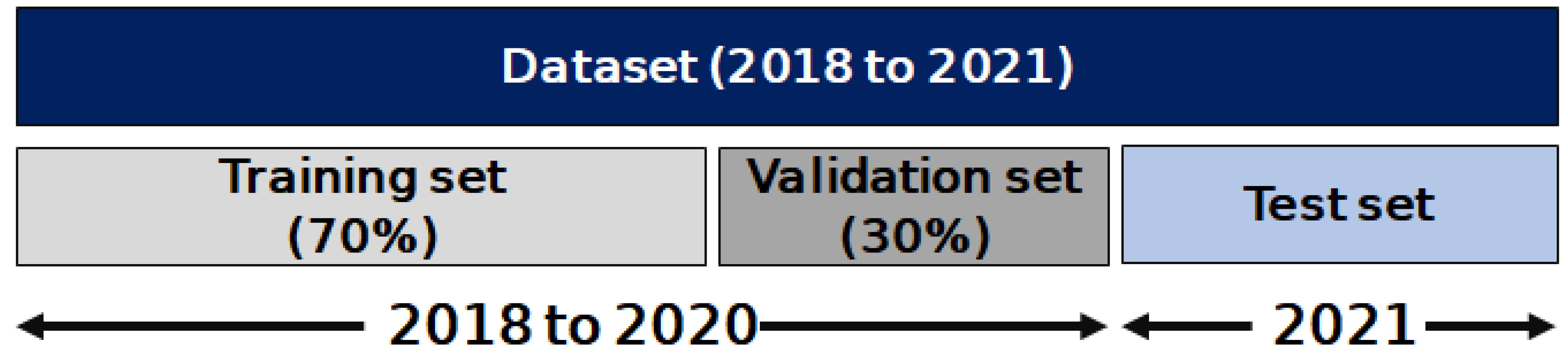
2.2. Data Collection

The visibility, meteorological, and air pollution data were collected in the Korean peninsula on an hourly basis from January 2018 to October 2022 (Figure 2, Table 1). In total, 33,600 datasets were collected (1400 days × 24 h). The visibility observation data were obtained from the Automated Synoptic Observing System (ASOS) of the Korea Meteorological Administration (KMA). A total of 94 ASOS ground-based observation sites are located in South Korea. The meteorological input parameters, including air temperature, surface pressure, wind speed, humidity, and precipitation data, were obtained from automatic weather stations (AWSs) of the KMA. Data were collected from 521 AWS observation sites during the study period. Furthermore, we calculated the temperature difference between the observation time and that measured before the observation times of 6, 12, and 24 h to account for the reduction in visibility from condensation owing to cooling (e.g., radiation fog, haze, and mist) [35,36]. Both ASOS and AWS measurement data were obtained from Open MET Data Portal of KMA (https://data.kma.go.kr/resources/html/en/ncdci.html, accessed on 6 February 2022). The air pollution input variables, such as the concentrations of ozone (O3), carbon monoxide (CO2), sulfur dioxide (SO2), nitrogen dioxide (NO2), and particulate matter (PM10, PM2.5), were collected from AirKorea observation sites (https://www.airkorea.or.kr/eng, accessed on 2 April 2022). Finally, the solar zenith angle (SZA) values for each location were calculated, based on the date, time, and location (longitude and latitude). The SZA was used as an input variable for the visibility estimation model to indirectly account for changes in radiation amounts because the SZA is dependent on the amount of radiation. Although the ASOS also measures the radiation amount, it could exhibit greater uncertainties following the gridding process when using a geostatistical approach.

2.3. Spatial Interpolation Process Using IDW

The spatial interpolation was carried out considering the Korean peninsula (longitude: 125.0° to 131.16°; latitude: 33.1° to 38.5°; only land pixels). The pixel size was determined based on the distance between a specific ASOS site and the nearest ASOS site thereto. As indicated in Table 2, the distances ranged from 0.05° to 1.8°, with an average value of 0.28°. In total, 30% (73%) of the ASOS sites were within 0.2° (0.3°) of the adjacent ASOS site. If the pixel size was set to 20 km, the visibility information of two or more ASOS observation points within 20 km could be located, and it was possible that the visibility values of the points would not be sufficiently reflected. A pixel size of 5 km was considered to be too fine because the distance between the observation points was approximately 0.2°. Thus, the pixel size was determined as 10 km.
IDW was adopted as the spatial interpolation model in this study. IDW has been used extensively in environmental studies [31,32,33,34]. IDW, which is a basic geostatistical process, is based on two assumptions: (1) The values of spatially adjacent points are similar owing to the common location factor and (2) The similarity decreases as the distance between the two points increases. IDW uses the weight between the observation point and the point to be estimated. In IDW interpolation, the power parameter (P), which is the exponent of the distance, indicates the significance of the surrounding points on the interpolated value. The typical value of P is 2 [33,34]. In this study, we attempted to determine appropriate P values for each parameter (the visibility, and meteorological and environmental input variables) by considering the distribution of the ground-based observations and pixel size. The P value for the visibility (ASOS sites) was set to 2, whereas the P values for the meteorological (AWS) and air pollution (AirKorea) input variables were set to 3. Figure 3 depicts the IDW interpolation results for each variable.

2.4. Construction of 2D Visibility Estimation Model Using RF Method

As the causes of low-visibility conditions are diverse owing to the complex geographical features and air pollution levels in South Korea [23,28], machine-learning-based visibility estimation models were constructed in each spatial location (spatial pixel). We used the RF model, which is an ensemble technique based on bagging and randomized node optimization [37]. The RF model averages a large collection of individual decision trees to reduce overfitting. Furthermore, the RF model has built-in feature importance called mean decrease accuracy (MDA) [37,38]. The MDA is a measure of the importance of each input variable, expressing how much accuracy the model loses by excluding each input variable. For each tree, the estimation accuracy using the original dataset was subtracted from that using the input variable permuted dataset, then the remainders were averaged over all trees in the forest, indicating the MDA. The resulting ‘MDA’ was an indicator of input variable importance with regard to its contribution to the estimation accuracy. In this study, we utilized the MDA values to evaluate the regional importance of each input variable in the 2D visibility estimation model (See Section 3.1). We performed the RF model training using the RandomForestRegressor from scikit-learn (version 1.0.2; NumFOCUS, Austin, TX, USA) [39] in Python (version 3.7.11; Python Software Foundation, Wilmington, DE, USA) [40]. The module includes various state-of-the-art machine-learning-based algorithms [39,41]. The RandomForestRegressor includes several hyperparameters, such as n_estimators (the number of trees in the forest) and max_features (the number of variables). The optimal hyperparameters should be selected for improved model performance [37,42]. We used the GridSearchCV function that is available from scikit-learn (version 1.0.2; NumFOCUS, Austin, TX, USA) to determine the optimal hyperparameters. The RF models in each spatial location were trained by optimizing the best hyperparameters. We randomly divided part of the collected dataset (2018 to 2020) into training (70%) and validation (30%) sets to construct the visibility estimation model (Figure 4). The dataset that was collected in 2021 was used as the test dataset, which was subsequently used to evaluate the performance of the visibility estimation model, as described in the following section.

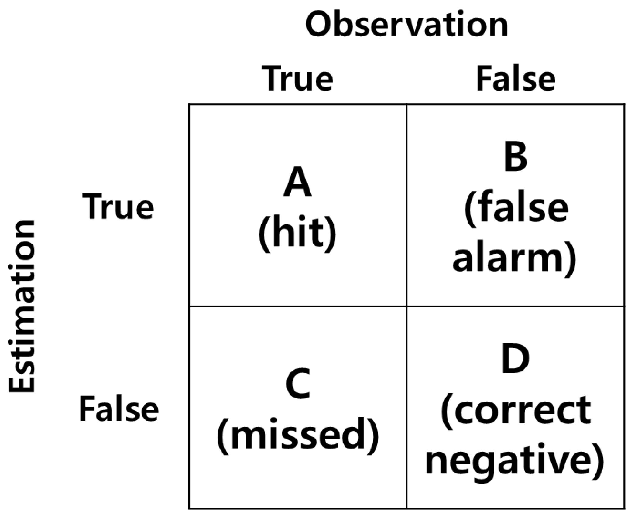
2.5. Assessment of Visibility Estimation Model

In this study, the values were estimated using a regression-based RF model. However, it was desirable to evaluate whether the model detected a specific visibility range effectively, as opposed to calculating the estimation error itself. Therefore, in this study, the performance of the visibility estimation model was evaluated based on the detection performance for each visibility range. The visibility ranges were classified into three groups (A: 10 to 20 km, B: 5 to 10 km, and C: 0 to 5 km) (Table 3), as suggested in previous studies [43,44,45]. Moreover, although we attempted to consider the visibility range between 0 and 1 km, it was excluded owing to few cases (<100) that were identified in South Korea during the test set period (January to October 2021).
Three statistical measures were used to evaluate the visibility estimation models: the recall, precision, and F1 score as used in the previous studies [46,47,48].
recall = A A + C
precision = A A + B
F 1   score = 2 × ( precision × recall ) precision + recall
In the above, A indicates a hit (corresponds to true positive), B is a false alarm (corresponds to false negative), C is a miss (corresponds to false positive), and D is a correct negative value (true negative), as illustrated in Figure 5. Recall indicates the ratio of the number of hits to the number of observed visibilities for each range. Precision is the ratio of the number of hits to the number of estimated visibilities for each range. F1 score is the harmonic mean of the precision and recall. The values of the recall, precision, and F1 score are 1 for the perfect model (for worst model, these values are at 0) [49].

2.6. Effect of Geostatistical Interpolation on Visibility Estimation Model

In this study, the ground-based data were spatially interpolated using the IDW method, following which visibility estimation models were constructed for each location (each pixel). However, it was necessary to investigate the performance of the visibility estimation model using spatial interpolation in locations with no observation sites. Thus, in this study, we focused on the effect of the gridded visibility on the model as it was the target variable and observation sites (ASOS) are sparsely distributed in South Korea. We constructed an additional visibility estimation model using spatially interpolated data without several ASOS stations to examine the effect of the spatial interpolation on the visibility estimation model. Subsequently, the visibility estimation error of the additionally constructed model (modeladdition) was compared with that of the originally constructed model (modeloriginal) in the locations where the ASOS site data were excluded from the geostatistical interpolation process. In this step, the visibility estimation errors (erroraddition and errororiginal) were calculated as the absolute mean bias value between the estimated and observed visibilities from the same test set. Table 4 lists the ASOS sites that were selected to investigate the effect of the spatial interpolation on the visibility model. Poor visibility conditions (<5 km) were frequently detected (>10,000 times) at these ASOS sites (Daegwallyeong, Inchen, and Imsil) over 10 years (2011 to 2020).

3. Results and Discussion

3.1. Variable Importance

Figure 6 depicts the importance of each input variable for the visibility estimation models that were located at the ASOS measurement sites. The mean decrease accuracies (MDAs) were spatially averaged over the ASOS measurement site locations. As reported in a previous study [13], the relative humidity and concentration of fine-mode aerosols (particularly PM2.5) had the highest variable importance, with the spatially averaged MDA values of 35% and 26%, respectively. The spatially averaged MDAs of the remaining input variables were less than 6%; however, the maximum MDAs of these input variables were over 5%, depending on the location in which the visibility estimation model was constructed. This implied that the influence of each input variable varied according to its location in the model. For example, the maximum MDA of the relative humidity was 49% on Heuksan Island, which is isolated from land with a background level of air pollutants, whereas that of PM2.5 on Heuksan Island was only 14%. In Seoul, which is the capital of South Korea, PM2.5 was the most crucial variable (MDA = 38%), and the MDA of the relative humidity was 32%. In the case of the SZA, the maximum MDA was 8% in Yang-san. Thus, our model could account for the regional characteristics of visibility in each location.

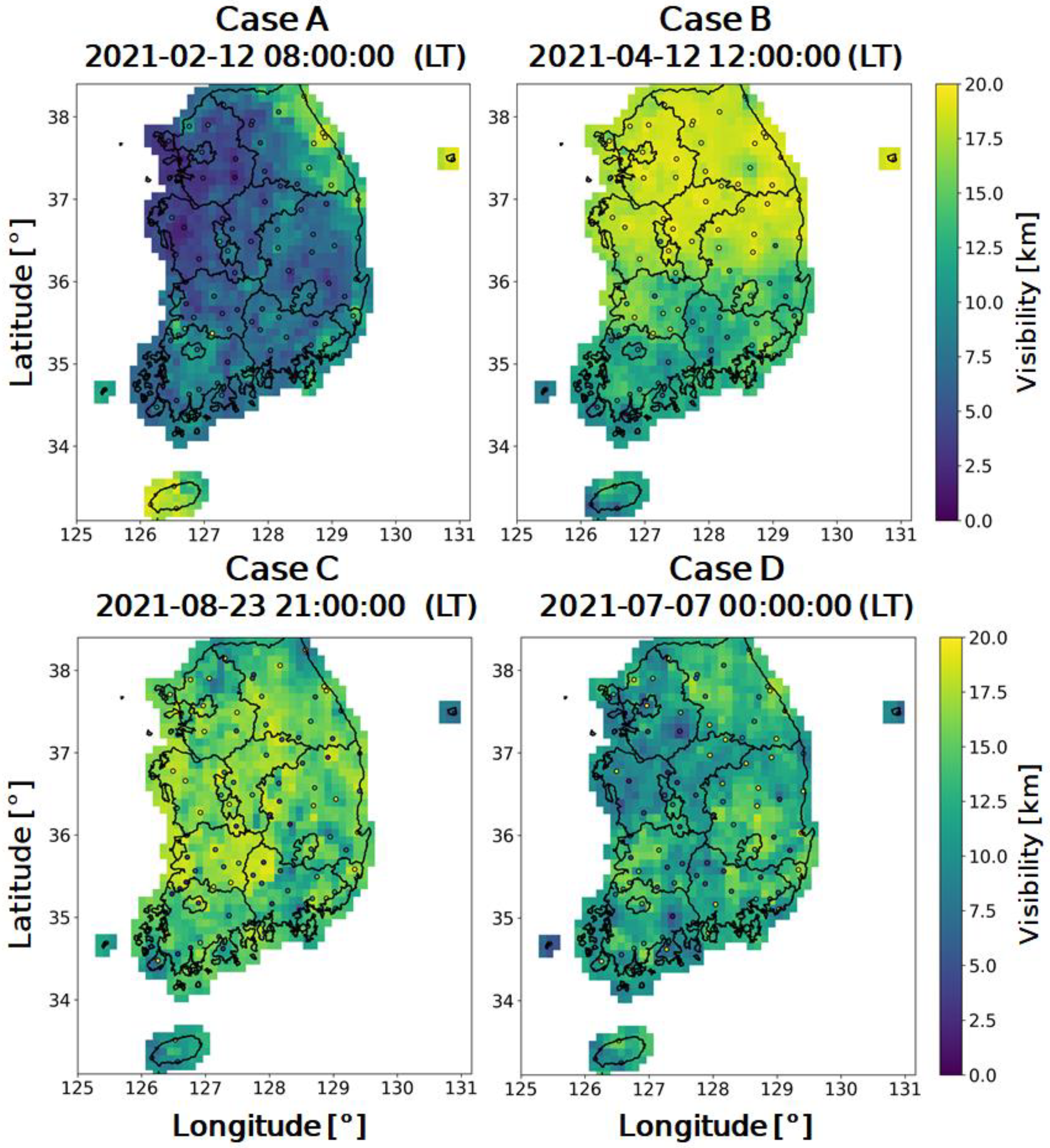
3.2. Visibility Estimation: Case Studies

In this study, spatial distributions of the estimated visibility values were investigated for four case studies including two well-estimated cases (Case A: 12:00 local time (LT) on 12 February 2021; Case B: 08:00 LT on 12 April 2021) and two wrongly-estimated cases (Case C: 21:00 LT on 23 August 2021; Case D: 00:00 LT on 7 July 2021). Figure 7 illustrates the spatial distributions of estimated visibility values using the constructed model on each location with 10 km pixel size for the cases A–D. The observed visibilities from the ASOS sites were also plotted to compare the estimated and observed values (Figure 7). As shown in the Figure 7, visibility values had various spatial distributions in South Korea.
For case A, 78% of the ASOS sites provided visibilities of less than 10 km (36% of sites: <5 km; 41% of sites: 5 ≤ visibility < 10 km), including haze cases over the entire Korean peninsula. For case B, the visibilities in the northern part of South Korea were greater than 10 km with clear weather conditions, whereas moderate visibility conditions were observed in the southern part of South Korea (24% of sites: visibility < 10 km). In general, the distributions of the observed and estimated values were strongly correlated for moderate- and low-visibility cases. The correlation coefficients between the estimated and observed values were determined as 0.73 and 0.81 for well-estimated cases (A and B), respectively. The average absolute mean bias between the estimated and observed values were 2.5 and 2.6 km, respectively.
Both wrongly-estimated cases (case C and D) included 50% of visibilities of less than 10 km (23% of sites: <5 km; 27% of sites: 5 ≤ visibility < 10 km). Case C indicated that our model overestimated visibility values while case D showed underestimation. The values of important input parameters (humidity, PM2.5, and PM10) were investigated for two cases. For case C, the humidity values ranged from 77% to 100% with an average value of 95%. However, low concentrations of PM2.5 and PM10 were found with average values of 5 µg/cm3 and 10 µg/cm3, respectively. It is thought that these low concentrations of PM2.5 and PM10 caused the model to estimate generally good visibility conditions. For case D, high PM2.5 and PM10 values were found with average (maximum) values of 19 µg/cm3 (83 µg/cm3) and 28 µg/cm3 (113 µg/cm3), respectively. It seems that these high aerosol concentrations caused the estimation of low visibility values in general. However, there were discrepancies between the estimated and observed visibilities in several locations for both cases. The causes of the discrepancies require more precise analysis in the future. However, it means that new important input variables should be introduced besides aerosol concentrations (PM10 and PM2.5) and humidity.

3.3. Effect of Geostatistical Interpolation on Visibility Estimation Model

In this study, spatial interpolation was performed to build a two-dimensional visibility estimation model so that visibility could be estimated even where visibility stations are not located. Therefore, as the distance from the visibility station increased, additional errors might be inherent due to the application of the geostatistical method. As described in Section 2.6, the visibility estimation error caused by spatial interpolation was investigated. The visibility estimation error of modeladditional was compared with that of modeloriginal in three sites where poor visibility events were frequent. The distance between the site and the nearest site was the farthest (0.29°) in Incheon, and the visibility estimation error increased by 470 m (Table 5). In Daegwallyeong, at a distance of 0.19°, the error increased by 180 m, indicating that the effect of the spatial interpolation on the visibility estimation error was not significant. However, the visibility estimation error for Imsil decreased by 60 m. Degradation of the visibility estimation model did not occur in limsil compared to Incheon and Daegwallyeong because ASOS sites are located within 0.3° from lmsil. When referencing the values of the adjacent ASOS stations, it appeared that degradation of the visibility estimation model did not occur. Therefore, the visibility estimation error with spatial interpolation is dependent on the distance from the adjacent ASOS site and number of nearby ASOS sites when visibility estimation models are constructed in locations with no ASOS sites. Hence, it appears that spatial interpolation may cause an additional visibility error of 500 m, as determined over the ASOS sites with frequent low visibility in South Korea. The degradation effect of the visibility estimation model with spatial interpolation appeared to be negligible for the nearest ASOS sites that were located within 0.2°. Therefore, it should be noted that additional visibility estimation errors (up to 500 m) can be caused by the spatial interpolation over the pixels located more than 0.2° from the actual visibility stations.

3.4. Assessment of Visibility Estimation Model

The visibility estimation models were evaluated based on the detection performance for three ranges of visibility values (range A: 10 to 20 km, range B: 5 to 10 km, and range C: 0 to 5 km) in South Korea using the test dataset (data period: January to October 2021) as shown in Figure 8. The statistical measures (recall, precision, and F1 score) were calculated for the pixels where a visibility estimation model was constructed, as described in Section 2.5. However, pixels in which visibility was observed in less than 120 cases were excluded from the performance test. The visibility counts were more than 120 for all pixels in ranges A and B, whereas several pixels of range C were excluded owing to the small number of cases (Figure 9). In addition, the performances of the model using training and validation datasets are in Figures S1 and S2 (Supplementary Materials).
In general, our model detected almost all good visibility conditions (range A: 10 to 20 km). For good visibility conditions, average values of all metrics (recall, precision, and F1 score) were close to 1.0, indicating the high visibility detection performance of our model for good visibility conditions.
For moderate visibility conditions (range B: 5 to 10 km), the spatial distributions of recall, precision, and F1 score were diverse. Moderate detection performance was observed in the middle-west part of South Korea for all metrics (average recall = 0.62, average precision = 0.61, average F1 score = 0.61). A relatively higher recall (average: 0.73) were detected in the northwestern part of South Korea, while low precision values (average: 0.42) were found in the region. The average F1 score was calculated as 0.52. It means that our model overestimated moderate visibility conditions in the northwestern part of South Korea. This might be explained by the lower number of cases in the moderate visibility conditions than in the other regions during the test period (Figure 8). Moreover, the recall values (average: 0.39) were low in the northeast region of South Korea (Gangwon Province), where air pollution measurement (AirKorea) sites are not evenly distributed. Therefore, it might be difficult to refer to air pollution information, including PM2.5, which is an important variable. Additional training with a longer data period and more measurement sites should be performed to improve the model detection performance in the region.
For the poor visibility case (range C: 0 to 5 km), the statistical measures (recall, precision, and F1 score) were calculated for the west-central part of South Korea (visibility counts >120 cases). In general, low recall values of an average of 0.25 were observed, however, high precision values (average: 0.79) were found. The average F1 score was 0.35. We found that our visibility estimation models tended to underestimate low-visibility conditions with low recall and high precision values, as demonstrated in the preliminary results. It is expected that the low-visibility estimation performance could be improved if additional model training was performed with more low-visibility cases using long-term data.

4. Conclusions

We have proposed a new model for estimating 2D visibility using a machine-learning technique. Point measurement data (visibility as well as meteorological and air pollution-based parameters) from South Korea were spatially interpolated using a geostatistical method. The gridded data were used to train the visibility estimation models for each location. The importance of the model input variables was distinct for each location, indicating that our model could account for the regional characteristics of visibility variation. Moreover, the effect of the spatial interpolation on the visibility estimation error was investigated. The model error was dependent on the location of adjacent visibility measurement sites. However, the error appeared to be negligible in locations where visibility observation sites were located within 0.2°, demonstrating the feasibility of the geostatistical method for visibility estimation. The performance of the model was preliminarily assessed using three measures (recall, precision, and F1 score). In general, the best performance was observed for the detection of good visibility conditions, whereas the preliminary performance for moderate and poor visibility conditions varied by region.
A regionally trained 2D visibility estimation model has been proposed in which the RF is used to investigate regional features of variable importance. In the future, other machine-learning techniques and deep learning can be applied to determine an optimal model for visibility estimation in each location. Furthermore, the accuracy of the model may be improved by collecting additional training data for moderate- and low-visibility conditions over a longer period. In addition, the spatial interpolation method used in this study is one of the common methods, suggested more than 20 years ago [50]. Recently, state-of-the-art geostatistical methods have been developed, such as the deep learning-based spatial interpolation method [51] and multiple Tensor-on-Tensor Regression [52,53]. The application of the latest approaches is expected to contribute to the improvement of the visibility estimation model. Finally, this study is the first to demonstrate a machine learning based model which estimates 2D visibility information that can be utilized for the safety of transportation (road, shipping, and aviation) and indirect diagnosis of air pollution.

Supplementary Materials

The following supporting information can be downloaded at: https://www.mdpi.com/article/10.3390/atmos13081233/s1, Figure S1: Recall, Precision, and F1 score of visibility estimation models in South Korea for three visibility ranges ((a) 0 to 5 km, (b) 5 to 10 km, and (c) 10 to 20 km) for the training set; Figure S2: Recall, Precision, and F1 score of visibility estimation models in South Korea for three visibility ranges ((a) 0 to 5 km, (b) 5 to 10 km, and (c) 10 to 20 km) for the validation set.

Author Contributions

Conceptualization, H.L. and W.C.; methodology, W.C.; writing, H.L. and W.C.; data curation, J.P. (Junsung Park), D.K., J.P. (Jeonghyun Park) and S.K. All authors have read and agreed to the published version of the manuscript.

Funding

This research was funded by the National Institute of Environment Research (NIER), funded by the Ministry of Environment (MOE) of the Republic of Korea (grant no. NIER-2022-01-02-118).

Institutional Review Board Statement

Not applicable.

Informed Consent Statement

Not applicable.

Data Availability Statement

Not applicable.

Conflicts of Interest

The authors declare no conflict of interest.

References

  1. Fita, L.; Polcher, J.; Giannaros, T.M.; Lorenz, T.; Milovac, J.; Sofiadis, G.; Katragkou, E.; Bastin, S. CORDEX-WRF v1.3: Development of a module for the Weather Research and Forecasting (WRF) model to support the CORDEX community. Geosci. Model Dev. 2019, 12, 1029–1066. [Google Scholar] [CrossRef] [Green Version]
  2. Cornejo-Bueno, S.; Casillas-Pérez, D.; Cornejo-Bueno, L.; Chidean, M.I.; Caamaño, A.J.; Sanz-Justo, J.; Casanova-Mateo, C.; Salcedo-Sanz, S. Persistence analysis and prediction of low-visibility events at Valladolid airport, Spain. Symmetry 2020, 12, 1045. [Google Scholar] [CrossRef]
  3. Xiao, S.; Wang, Q.; Cao, J.; Huang, R.-J.; Chen, W.; Han, Y.; Xu, H.; Liu, S.; Zhou, Y.; Wang, P. Long-term trends in visibility and impacts of aerosol composition on visibility impairment in Baoji, China. Atmos. Res. 2014, 149, 88–95. [Google Scholar] [CrossRef]
  4. Babari, R.; Hautière, N.; Dumont, É.; Paparoditis, N.; Misener, J. Visibility monitoring using conventional roadside cameras–Emerging applications. Transp. Res. C Emerg. Technol. 2012, 22, 17–28. [Google Scholar] [CrossRef] [Green Version]
  5. Gultepe, I.; Sharman, R.; Williams, P.D.; Zhou, B.; Ellrod, G.; Minnis, P.; Trier, S.; Griffin, S.; Yum, S.; Gharabaghi, B. A review of high impact weather for aviation meteorology. Pure Appl. Geophys. 2019, 176, 1869–1921. [Google Scholar] [CrossRef]
  6. Shan, Y.; Zhang, R.; Gultepe, I.; Zhang, Y.; Li, M.; Wang, Y. Gridded visibility products over marine environments based on artificial neural network analysis. Appl. Sci. 2019, 9, 4487. [Google Scholar] [CrossRef] [Green Version]
  7. U.S. Department of Transportation Federal Highway Administration. Low Visibility. Available online: https://ops.fhwa.dot.gov/weather/weather_events/low_visibility.htm (accessed on 1 June 2022).
  8. Hyslop, N.P. Impaired visibility: The air pollution people see. Atmos. Environ. 2009, 43, 182–195. [Google Scholar] [CrossRef]
  9. Stocker, T. Climate Change 2013: The Physical Science Basis: Working Group I Contribution to the Fifth Assessment Report of the Intergovernmental Panel on Climate Change; Cambridge University Press: Cambridge, UK, 2014. [Google Scholar]
  10. Singh, A.; George, J.P.; Iyengar, G.R. Prediction of fog/visibility over India using NWP Model. J. Earth Syst. Sci. 2018, 127, 26. [Google Scholar] [CrossRef] [Green Version]
  11. Huang, H.; Zhang, G. Case Studies of Low-Visibility Forecasting in Falling Snow with WRF Model. J. Geophys. Res. Atmos. 2017, 122, 862–874. [Google Scholar] [CrossRef]
  12. Kim, M.; Lee, K.; Lee, Y.H. Visibility data assimilation and prediction using an observation network in South Korea. Pure Appl. Geophys. 2020, 177, 1125–1141. [Google Scholar] [CrossRef]
  13. Kim, B.-Y.; Cha, J.W.; Chang, K.-H.; Lee, C. Visibility Prediction over South Korea Based on Random Forest. Atmosphere 2021, 12, 552. [Google Scholar] [CrossRef]
  14. Ortega, L.C.; Otero, L.D.; Solomon, M.; Otero, C.E.; Fabregas, A. Deep learning models for visibility forecasting using climatological data. Int. J. Forecast. 2022, in press. [Google Scholar] [CrossRef]
  15. Chaabani, H.; Werghi, N.; Kamoun, F.; Taha, B.; Outay, F. Estimating meteorological visibility range under foggy weather conditions: A deep learning approach. Procedia Comput. Sci. 2018, 141, 478–483. [Google Scholar] [CrossRef]
  16. Palvanov, A.; Cho, Y.I. Visnet: Deep convolutional neural networks for forecasting atmospheric visibility. Sensors 2019, 19, 1343. [Google Scholar] [CrossRef] [Green Version]
  17. Li, S.; Fu, H.; Lo, W.-L. Meteorological visibility evaluation on webcam weather image using deep learning features. Int. J. Comput. Theory Eng. 2017, 9, 455–461. [Google Scholar] [CrossRef] [Green Version]
  18. You, Y.; Lu, C.; Wang, W.; Tang, C.-K. Relative CNN-RNN: Learning relative atmospheric visibility from images. IEEE Trans. Image Processing ITIP 2018, 28, 45–55. [Google Scholar] [CrossRef] [PubMed]
  19. Song, M.; Han, X.; Liu, X.F.; Li, Q. Visibility estimation via deep label distribution learning in cloud environment. J. Cloud Comput. 2021, 10, 46. [Google Scholar] [CrossRef]
  20. Lo, W.L.; Zhu, M.; Fu, H. Meteorology visibility estimation by using multi-support vector regression method. J. Adv. Inf. Technol. 2020, 11, 40–47. [Google Scholar] [CrossRef]
  21. Lo, W.L.; Chung, H.S.H.; Fu, H. Experimental evaluation of pso based transfer learning method for meteorological visibility estimation. Atmosphere 2021, 12, 828. [Google Scholar] [CrossRef]
  22. Li, J.; Lo, W.L.; Fu, H.; Chung, H.S.H. A transfer learning method for meteorological visibility estimation based on feature fusion method. Appl. Sci. 2021, 11, 997. [Google Scholar] [CrossRef]
  23. Kim, J.; Kim, S.H.; Seo, H.W.; Wang, Y.V.; Lee, Y.G. Meteorological characteristics of fog events in Korean smart cities and machine learning based visibility estimation. Atmos. Res. 2022, 275, 106239. [Google Scholar] [CrossRef]
  24. Bremnes, J.B.; Michaelides, S.C. Probabilistic visibility forecasting using neural networks. In Fog and Boundary Layer Clouds: Fog Visibility and Forecasting; Springer: Berlin/Heidelberg, Germany, 2007; pp. 1365–1381. [Google Scholar]
  25. Marzban, C.; Leyton, S.; Colman, B. Ceiling and visibility forecasts via neural networks. Weather. Forecast. 2007, 22, 466–479. [Google Scholar] [CrossRef] [Green Version]
  26. Ortega, L.; Otero, L.D.; Otero, C. Application of machine learning algorithms for visibility classification. In Proceedings of the 2019 IEEE International Systems Conference (SysCon), Orlando, FL, USA, 8–11 April 2019; pp. 1–5. [Google Scholar]
  27. Bari, D.; Ouagabi, A. Machine-learning regression applied to diagnose horizontal visibility from mesoscale NWP model forecasts. SN Appl. Sci. 2020, 2, 556. [Google Scholar] [CrossRef] [Green Version]
  28. Chung, Y.; Kim, H.; Yoon, M. Observations of visibility and chemical compositions related to fog, mist and haze in South Korea. Water Air Soil Pollut. 1999, 111, 139–157. [Google Scholar] [CrossRef]
  29. Lee, S.H.; Kim, D.H.; Lee, H.W. Satellite-based assessment of the impact of sea-surface winds on regional atmospheric circulations over the Korean Peninsula. Int. J. Remote Sens. 2008, 29, 331–354. [Google Scholar] [CrossRef]
  30. Choi, S.W.; Kim, S.S. The past and current status of endangered butterflies in Korea. Entomol. Sci. 2012, 15, 1–12. [Google Scholar] [CrossRef]
  31. Jha, D.K.; Sabesan, M.; Das, A.; Vinithkumar, N.; Kirubagaran, R. Evaluation of Interpolation Technique for Air Quality Parameters in Port Blair, India. Univers. J. Environ. 2011, 1, 301–310. [Google Scholar]
  32. Gómez-Losada, Á.; Santos, F.M.; Gibert, K.; Pires, J.C. A data science approach for spatiotemporal modelling of low and resident air pollution in Madrid (Spain): Implications for epidemiological studies. Comput. Environ. Urban Syst. 2019, 75, 1–11. [Google Scholar] [CrossRef]
  33. Shukla, K.; Kumar, P.; Mann, G.S.; Khare, M. Mapping spatial distribution of particulate matter using Kriging and Inverse Distance Weighting at supersites of megacity Delhi. Sustain. Cities Soc. 2020, 54, 101997. [Google Scholar] [CrossRef]
  34. Tella, A.; Balogun, A.-L. Prediction of ambient PM10 concentration in Malaysian cities using geostatistical analyses. J. Geo Spat. Sci. Technol. 2021, 1, 115–127. [Google Scholar]
  35. Duynkerke, P.G. Radiation fog: A comparison of model simulation with detailed observations. Mon. Weather Rev. 1991, 119, 324–341. [Google Scholar] [CrossRef] [Green Version]
  36. Prusov, V.; Doroshenko, A. Computational Techniques for Modeling Atmospheric Processes; IGI Global: Hershey, PA, USA, 2017. [Google Scholar]
  37. Breiman, L. Random forests. Mach. Learn. 2001, 45, 5–32. [Google Scholar] [CrossRef] [Green Version]
  38. Louppe, G.; Wehenkel, L.; Sutera, A.; Geurts, P. Understanding variable importances in forests of randomized trees. In Advances in Neural Information Processing Systems; MIT Press: Cambridge, MA, USA, 2013. [Google Scholar]
  39. Pedregosa, F.; Varoquaux, G.; Gramfort, A.; Michel, V.; Thirion, B.; Grisel, O.; Blondel, M.; Prettenhofer, P.; Weiss, R.; Dubourg, V. Scikit-learn: Machine learning in Python. J. Mach. Learn. Res. 2011, 12, 2825–2830. [Google Scholar]
  40. Van, R.G.; Drake, F. Python 3 Reference Manual; CreateSpace: Scotts Valley, CA, USA, 2009. [Google Scholar]
  41. Torre-Tojal, L.; Bastarrika, A.; Boyano, A.; Lopez-Guede, J.M.; Graña, M. Above-ground biomass estimation from LiDAR data using random forest algorithms. J. Comput. Sci. 2022, 58, 101517. [Google Scholar] [CrossRef]
  42. Mutanga, O.; Adam, E.; Cho, M.A. High density biomass estimation for wetland vegetation using WorldView-2 imagery and random forest regression algorithm. Int. J. Appl. Earth Obs. Geoinf. 2012, 18, 399–406. [Google Scholar] [CrossRef]
  43. Kuo, C.-Y.; Cheng, F.-C.; Chang, S.-Y.; Lin, C.-Y.; Chou, C.C.; Chou, C.-H.; Lin, Y.-R. Analysis of the major factors affecting the visibility degradation in two stations. J. Air Waste Manag. Assoc. 2013, 63, 433–441. [Google Scholar] [CrossRef] [Green Version]
  44. Elias, T.; Jolivet, D.; Mazoyer, M.; Dupont, J.-C. Favourable and Unfavourable Scenarii of Radiative Fog Formation Defined by Ground-Based and Satellite Observation Data. Aerosol Air Qual. Res. 2018, 18, 145–164. [Google Scholar] [CrossRef] [Green Version]
  45. Sun, X.; Zhao, T.; Liu, D.; Gong, S.; Xu, J.; Ma, X. Quantifying the influences of PM2.5 and relative humidity on change of atmospheric visibility over recent winters in an urban area of East China. Atmosphere 2020, 11, 461. [Google Scholar] [CrossRef]
  46. Ghorbanzadeh, O.; Tiede, D.; Dabiri, Z.; Sudmanns, M.; Lang, S. Dwelling extraction in refugee camps using CNN-first experiences and lessons learnt. Int. Arch. Photogramm. Remote Sens. Spat. Inf. Sci. 2018, 42, 161–166. [Google Scholar] [CrossRef] [Green Version]
  47. Lathifah, S.N.; Nhita, F.; Aditsania, A.; Saepudin, D. Rainfall Forecasting using the Classification and Regression Tree (CART) Algorithm and Adaptive Synthetic Sampling (Study Case: Bandung Regency). In Proceedings of the 2019 7th International Conference on Information and Communication Technology (ICoICT), Kuala Lumpur, Malaysia, 24–26 July 2019; pp. 1–5. [Google Scholar]
  48. Krishna, P.R.; Ahammad, P.; Sethuraman, R. Hybrid Prediction Models for Rainfall Forecasting. Ann. Rom. Soc. Cell Biol. 2021, 25, 40–46. [Google Scholar]
  49. Manimannan, G.; Priya, R.L.; Reena, K.J.; Priya, S.K. Climate Changes of Tamilnadu Based on Rainfall Data Using Data Mining Model Evaluation and Cross Validation. IOSR J. Comput. Eng. 2018, 20, 32–38. [Google Scholar]
  50. New, M.; Hulme, M.; Jones, P. Representing twentieth-century space–time climate variability. Part II: Development of 1901–96 monthly grids of terrestrial surface climate. J. Clim. 2000, 13, 2217–2238. [Google Scholar] [CrossRef]
  51. Kirkwood, C.; Economou, T.; Pugeault, N.; Odbert, H. Bayesian deep learning for spatial interpolation in the presence of auxiliary information. Math. Geosci. 2022, 54, 507–531. [Google Scholar] [CrossRef]
  52. Gahrooei, M.R.; Yan, H.; Paynabar, K.; Shi, J. Multiple tensor-on-tensor regression: An approach for modeling processes with heterogeneous sources of data. Technometrics 2021, 63, 147–159. [Google Scholar] [CrossRef]
  53. Rajput, M.; Gahrooei, M.R.; Augenbroe, G. A statistical model of the spatial variability of weather for use in building simulation practice. Build. Environ. 2021, 206, 108331. [Google Scholar] [CrossRef]
Figure 1. Flowchart of development of visibility estimation model.
Atmosphere 13 01233 g001
Figure 2. Locations of (a) ASOS, (b) AWS, and (c) AirKorea observation sites in South Korea.
Atmosphere 13 01233 g002
Figure 3. IDW interpolation results and ground-based observations of (a) visibility, (b) humidity, (c) pressure, (d) temperature, (e) precipitation, (f) wind speed, (g) PM2.5, (h) PM10, (i) O3, (j) NO2, (k) CO, and (l) SO2 concentrations. The circle symbols indicate observed values.
Atmosphere 13 01233 g003
Figure 4. Division of dataset: training, validation, and test sets.
Atmosphere 13 01233 g004
Figure 5. Contingency table used to estimate visibility detection performance.
Atmosphere 13 01233 g005
Figure 6. Spatially averaged variable importance (mean decrease accuracy) of visibility estimation model. The error bar indicates the standard deviations.
Atmosphere 13 01233 g006
Figure 7. Estimated visibility maps at 12:00 LT on 12 February 2021 (case A), 08:00 LT on 12 April 2021 (case B), 21:00 LT on 23 August 2021 (case C), and 00:00 LT on 7 July 2021 (case D). The circle symbols indicate observed visibilities from ASOS at the same times.
Atmosphere 13 01233 g007
Figure 8. Recall, Precision, and F1 score of visibility estimation models in South Korea for three visibility ranges ((a) 0 to 5 km, (b) 5 to 10 km, and (c) 10 to 20 km) for period from January to October 2021 (test set).
Atmosphere 13 01233 g008
Figure 9. Visibility counts according to visibility ranges (AC) for period from January to October 2021.
Atmosphere 13 01233 g009
Table 1. Sites, units, and temporal resolutions of target variable (visibility) and input variables (meteorological and air pollution).
TypeSiteParameter (Abbreviation)UnitTemporal Resolution
Target variableASOS a
(KMA b)
VisibilitykmHourly
Meteorological input variablesAWS c
(KMA)
Air temperature (T)°C
Pressure (P)hPa
Wind speed (WS)m/s
Humidity (Humid)%
Precipitation (Precip)mm
Delta temperature (ΔT)
ΔT24, ΔT12, ΔT06
°C
Air pollution input variablesAirKorea
(KECO d)
O3 concentration (O3)ppm
CO concentration (CO)ppm
SO2 concentration (SO2)ppm
NO2 concentration (NO2)ppm
PM10 concentration (PM10)µg/cm3
PM2.5 concentration (PM2.5)µg/cm3
Other input parametersSolar zenith angle (SZA)° (degrees)
a ASOS: Automated Synoptic Observing System. b KMA: Korea Meteorological Administration. c AWS: Automatic weather station. d KECO: Korea Environment Corporation.
Table 2. Number of ASOS sites and statistical values of distance between specific ASOS site and nearest site.
Number of ASOS SitesStatistical Values
Total94 sitesMinimum0.05°
Distance ≤ 0.05°2 sitesMaximum1.8°
Distance ≤ 0.1°4 sitesAverage0.28°
Distance ≤ 0.2°28 sitesStandard deviation0.23°
Distance ≤ 0.3°69 sites
Distance ≤ 0.4°87 sites
Table 3. Definitions of visibility ranges.
Visibility RangeNote
A10 to 20 kmGood visibility (clear air)
B5 to 10 kmModerate visibility
C0 to 5 kmPoor visibility
Table 4. Summary of ASOS sites for investigating effect of spatial interpolation.
Station Name (Code)Latitude LongitudePoor Visibility CasesNotes
Daegwallyeong (100)37.6771°128.7183°10,981- Coastal area
AirKorea sites are sparsely distributed
Incheon (112)37.4776°126.6244°12,242- Coastal areaAir
Korea sites are sparsely distributed
Imsil (244)35.6120°127.2856°12,242- Inland area
Table 5. Summary of visibility estimation errors of modeloriginal and modeladditional.
Site NameDistance between Site and Nearest SiteAbsolute Mean Bias (Correlation Coefficient)
ErrororiginalErroradditional
Daegwallyeong0.19°1.56 km (0.83)1.74 km (0.81)
Incheon0.29°1.45 km (0.93)1.92 km (0.91)
Imsil0.22°1.81 km (0.79)1.75 km (0.78)
Publisher’s Note: MDPI stays neutral with regard to jurisdictional claims in published maps and institutional affiliations.

