Article

Long-Term Variations of Meteorological and Precursor Influences on Ground Ozone Concentrations in Jinan, North China Plain, from 2010 to 2020

1
School of Environmental Science and Engineering, Qilu University of Technology (Shandong Academy of Sciences), Jinan 250300, China
2
Shandong Provincical Jinan Eco-Environment Monitoring Center, Jinan 250102, China
*
Author to whom correspondence should be addressed.
Atmosphere 2022, 13(6), 994; https://doi.org/10.3390/atmos13060994
Submission received: 18 May 2022 / Revised: 9 June 2022 / Accepted: 17 June 2022 / Published: 20 June 2022

Abstract

:
Ground-level ozone (O3) pollution in the North China Plain has become a serious environmental problem over the last few decades. The influence of anthropogenic emissions and meteorological conditions on ozone trends have become the focus of widespread research. We studied the long-term ozone trends at urban and suburban sites in a typical city in North China and quantified the contributions of anthropogenic and meteorological factors. The results show that urban O3 increased and suburban O3 decreased from 2010 to 2020. The annual 90th percentile of the maximum daily 8-h average of ozone in urban areas increased by 3.01 μgm−3year−1 and, in suburban areas, it decreased by 3.74 μgm−3year−1. In contrast to the meteorological contributions, anthropogenic impacts are the decisive reason for the different ozone trends in urban and suburban areas. The rapid decline in nitrogen oxides (NOX) in urban and suburban areas has had various effects. In urban areas, this leads to a weaker titration of NOX and enhanced O3 formation, while in suburban areas, this weakens the photochemical production of O3. Sensitivity analysis shows that the O3 formation regime is in a transition state in both the urban and suburban areas. However, this tends to be limited to volatile organic compounds (VOCs) in urban areas and to NOX in suburban areas. One reasonable approach to controlling ozone pollution should be to reduce nitrogen oxide emissions while strengthening the control of VOCs.

1. Introduction

Tropospheric ozone (O3) is an important contributor to atmospheric oxidation and can be harmful to human health and the Earth’s ecosystems at high concentrations [1,2,3,4,5]. Surface ozone mainly comes from the photochemical reactions of volatile organic compounds (VOCs) with nitrogen oxides (NOX), and there is a strong non-linear relationship between ozone and precursor emissions [6,7,8,9,10,11]. A significant improvement in ambient air quality has been reported widely in China, in response to stringent emission control measures. The Clean Air Action Plan (CAAP), launched in China in 2013, has led to rapid reductions in nitrogen dioxide (NO2), sulfur dioxide (SO2), and particulate matter concentrations [12]. However, it is worth noting that ozone pollution remains serious and even continues to worsen [8,13,14,15].
Ozone shows a continuous growth trend in urban regions in China, especially in developed regions, such as Beijing–Tianjin–Hebei (BTH), the Yangtze River Delta (YRD), and the Pearl River Delta (PRD) [14,16]. About 30% of these sites showed an increasing trend of more than 6.4 μgm−3year−1 (3.0 ppb·year−1) from 2013 to 2019 [17]. The average annual growth rate of O3 was found at a rate of 1.35–8.14 μgm−3year−1 from 2013 to 2017, in the YRD region [18]. The highest-increasing trend of O3 was 0.649 μgm−3year−1 from 2006 to 2019, in the PRD region [19]. The maximum daily 8h average of ozone (MDA8 O3) showed an average rate of 7.06 μgm−3year−1 from 2013 to 2017 in the BTH region, which is located in the North China Plain (NCP), making it one of the most serious ozone pollution areas in China [20]. The reasons for these increasing trends are not fully understood and the existing explanations are controversial. It is worth noting that a slight decrease in maximum O3 concentrations was found in the Beijing regional site from 2014 to 2020 [21]. Ozone may have shown different trends in urban and suburban areas due to the different precursor emissions, as well as meteorological factors [22,23]. Most of the abovementioned studies on the recent ozone changes in China have been conducted on an urban scale. However, precise studies regarding suburban or more remote sites in specific cities are lacking.
Previous studies have been conducted to investigate the positive trend of ozone pollution through observations and models. The changes in precursor emissions, meteorology, and climate are all reported factors for the increasing ozone trends in China [15,24,25,26,27]. In addition, the effect of reduced particulate matter concentrations on ozone pollution is controversial [11,13,18,28,29], Some researchers have also investigated the enhanced ozone trend in a regional context and in terms of atmospheric oxidation [30,31]. The ozone formation potentials of different VOCs are also used as an important impact factor, to resolve the issue of O3 pollution and long-term changes [32]. However, the driving factors of ozone trends in urban and regional sites in North China are still unclear and should be investigated further.
Understanding the trends and the variability of ozone in urban and suburban areas may help tackle the ozone pollution problems emerging in the NCP region. This study conducted long-term ozone and relevant parameter observations from 2010 to 2020 at urban and suburban locations in Jinan, a typical capital city in the central NCP. A stepwise multiple linear regression model was used to calculate the contributions of anthropogenic emissions and meteorological changes to ozone pollution and to explore the main ozone pollution-influencing factors in North China. The changes in NOX and VOCs emissions and O3-NOX-VOCs sensitivity were inferred on the basis of the tropospheric NO2 and formaldehyde (HCHO) vertical columns in the ozone monitoring instrument’s (OMI) remote-sensing data. Finally, we put forward some specific O3 pollution control measures, according to the different O3 trends and O3 formation mechanisms in urban and suburban areas.

2. Materials and Methods

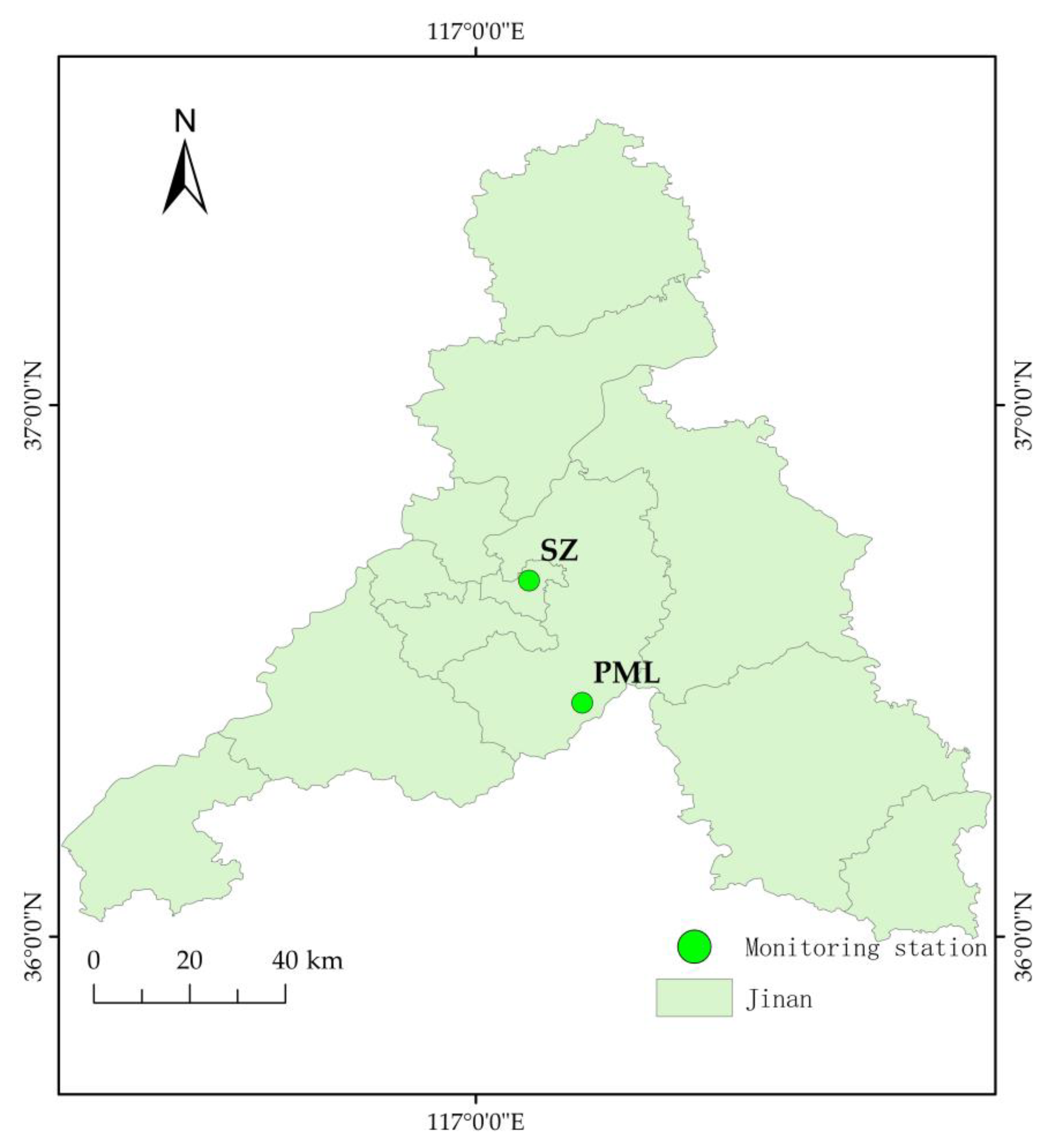
2.1. Study Site and Ozone Observations

Hourly concentrations of O3, NOX, CO, and particulate matter (PM10 and PM2.5) were obtained from the National Urban Air Quality Real-Time Publishing Platform (https://air.cnemc.cn:18007/ (accessed on 30 September 2021)) and the Jinan Municipal Ecological and Environmental Monitoring Center (http://jnepb.jinan.gov.cn/index.html (accessed on 30 September 2021)). The accuracy of this monitoring data is better than ±5%. All data were collected from 1 January 2010 to 31 December 2020 at two sites in Jinan, a central city in the NCP region of China. The city station (SZ) is a typical urban monitoring site, located at the Jinan air quality monitoring station (117.1° E, 36.67° N). The Paomaling (PML) site is a suburban site located in the Paomaling scenic area, 27 km away from downtown Jinan (117.2° E, 36.44° N). Figure 1 shows the locations of the monitoring sites in the urban and suburban areas. Ozone mass concentrations were reported in units of μgm−3. All data were preprocessed to eliminate the unreliable observed outliers. This was performed in the same way as in previous studies, using the z-score method to normalize the time series of hourly concentrations at specific monitoring sites [21,33]. The z-score is also known as the standard score and represents the process of dividing the difference between a score and the mean by the standard deviation:
zt = (t−μ)/σ
where t is a specific score, μ is the mean and σ is the standard deviation.
The data were removed in the following criteria: (1) having an absolute z score of larger than 4 (|zt| > 4), and (2) having a ratio of the value to its centered rolling mean of 3 (RM3), which is larger than 2 (zt/RM3(zt) > 2).

2.2. Ozone Metrics

Several metrics (Table 1) are used to characterize ozone pollution. These indicators include standard statistics, such as MDA8, which is widely used in many regions, including the United States, Europe, and China, to assess ozone air quality and examine the human health response to ozone exposure [21,34]. Here, the 90th percentile of MDA8 is calculated, to characterize the annual variability of ozone. The daily 10th percentile, 50th percentile, and 90th percentile 1-h ozone levels were used to characterize the background, mean, and high concentrations. All metrics were derived from hourly measurements, which were screened (Table 1).
We used the Chinese air quality standard, GB3095-2012, in Table 2 for the evaluation of ozone pollution.

2.3. Trend Analyses

Two types of analysis methods were used in this study. First, the trend was obtained using the least-squares regression equation when the anomalies were disturbed, and the significance was determined by Spearman’s order correlation coefficient, which was applied to ozone trend analysis in previous studies and recommended by the Chinese Ministry of Ecology and Environment [35]. Secondly, when there was more interference by outliers and the trend change was not obvious, the Sen + Mann–Kendall (Sen + MK) method was employed to assess the trend using the Sen method and test the significance using the MK test. The MK test has the advantage of not being disturbed by outliers and does not require the sample to follow a certain distribution, which means that it is widely used in hydrology, meteorology, and other studies, and is also used by scholars for the study of ozone [21]. This method is mainly used in the current paper to evaluate the anthropogenic and meteorological contributions via meteorological stepwise multiple linear regression (MLR).

2.4. Stepwise Multiple Linear Regression (MLR) Model

To quantify the role of meteorology in the ozone trends from 2010 to 2020, we used the stepwise MLR model, which relates the month-to-month changes in MDA8 O3 to the changes in meteorological variables. MLR builds meteorological data using the NASA Modern Research and Applications Retrospective Analysis, Version 2 (MERRA-2) product [36]. The spatial resolution of MERRA-2 data is 0.5 latitude × 0.625 longitude.
Since the meteorological parameters of ground-based observations were insufficient for the MLR model, we performed a stepwise fit analysis of the area-averaged data of the meteorological parameters of MERRA-2 and the observed daily MDA8 O3 for the studied geographical interval, from 2010 to 2020. We verified the validity of the MERRA-2 data by using some of the meteorological data from ground-based observations. We found that the Pearson correlation coefficients of temperature and relative humidity between MERRA-2 and the ground-based observations are 0.89 and 0.71, respectively (Figure S1). Thus, the MERRA-2 meteorological parameters were used in this study.
In Figure S1, we verify the validity of the MERRA-2 data by using some of the meteorological data from our ground-based observations. Nine MERRA-2 meteorological variables were screened on the basis of other researchers’ methods and were considered ozone covariates [12,14]. This includes the daily maximum 2-m air temperature (Tmax), 10-m east wind (U10) and 10-m north wind (V10), total cloud area fraction (TC), area mean of total surface precipitation (TP), sea level pressure (SLP), relative humidity (RH), surface incident shortwave flux (clear sky) (SF), and surface wind speed (WS). The meteorological data used for MLR are averaged over 24 h of data per day, except for Tmax and TC. TC is the average value from 8 a.m. to 8 p.m., local time.
To avoid over-fitting, only four dominant meteorological parameters were screened as fitting variables for the final regression model, to quantify the role of meteorological changes from 2010 to 2020. The variables were selected based on their individual contribution to the regression ozone and were statistically significant, above the 95% confidence level required for the MLR model. The MLR model was subjected to an ANOVA to test its significance, and the degree of fit was expressed by the coefficient of determination R2. Finally, the meteorological means were substituted into the MLR model, and the residuals between the resulting estimates and the true means were non-meteorological effects (anthropogenic effects); here, the trend estimates and significance tests were performed using the Sen + MK test.

2.5. Satellite Observations

Due to the lack of observational data on precursor VOCs and the lag in emission inventory data, this study uses the continuous global observations of two species of O3 precursors provided by the satellite spectrometer OMI to indicate NOX changes, using the nitrogen dioxide (NO2) column concentration changes and VOCs concentration changes via HCHO column concentration changes. OMI is a nadir-viewing spectrometer that was launched onboard the NASA Earth Observing Satellite Aura into a sun-synchronous orbit in 2004.
The data used for NO2 is the Level-3 daily global gridded (0.25° × 0.25°) nitrogen dioxide product (OMNO2d). The OMNO2d data product is a Level-3 gridded product, in which high-quality pixel-level data are combined and averaged into a 0.25° × 0.25° global grid. The data used for HCHO are from the OMI/Aura formaldehyde (HCHO) total HCHO column daily L3-weighted average global 0.1° latitude/longitude grid (OMHCHOd). The formaldehyde values in each file are the average of the 0.1° × 0.1° grid cells of the total HCHO column for one day of cloud screening.
We downloaded the satellite data from OMI at Giovanni (The Bridge Between Data and Science, v 4.36, https://giovanni.gsfc.nasa.gov/giovanni/ (accessed on 30 September 2021)). We selected single pixels of the urban and suburban sites and screened the abnormal values. About 900 pieces of useful data were used in this study.

3. Results and Discussions

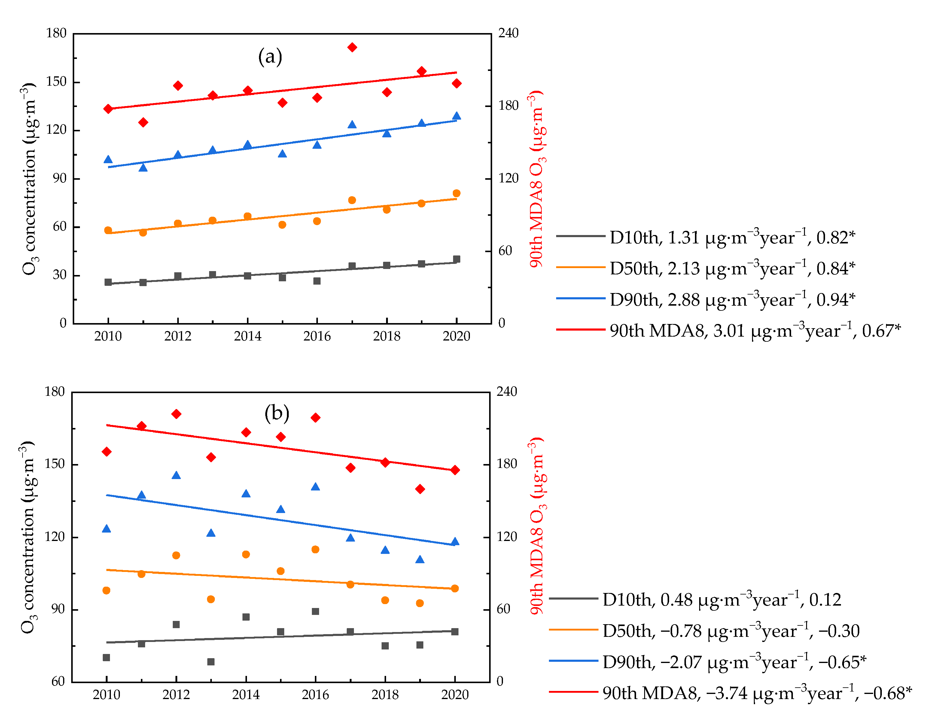
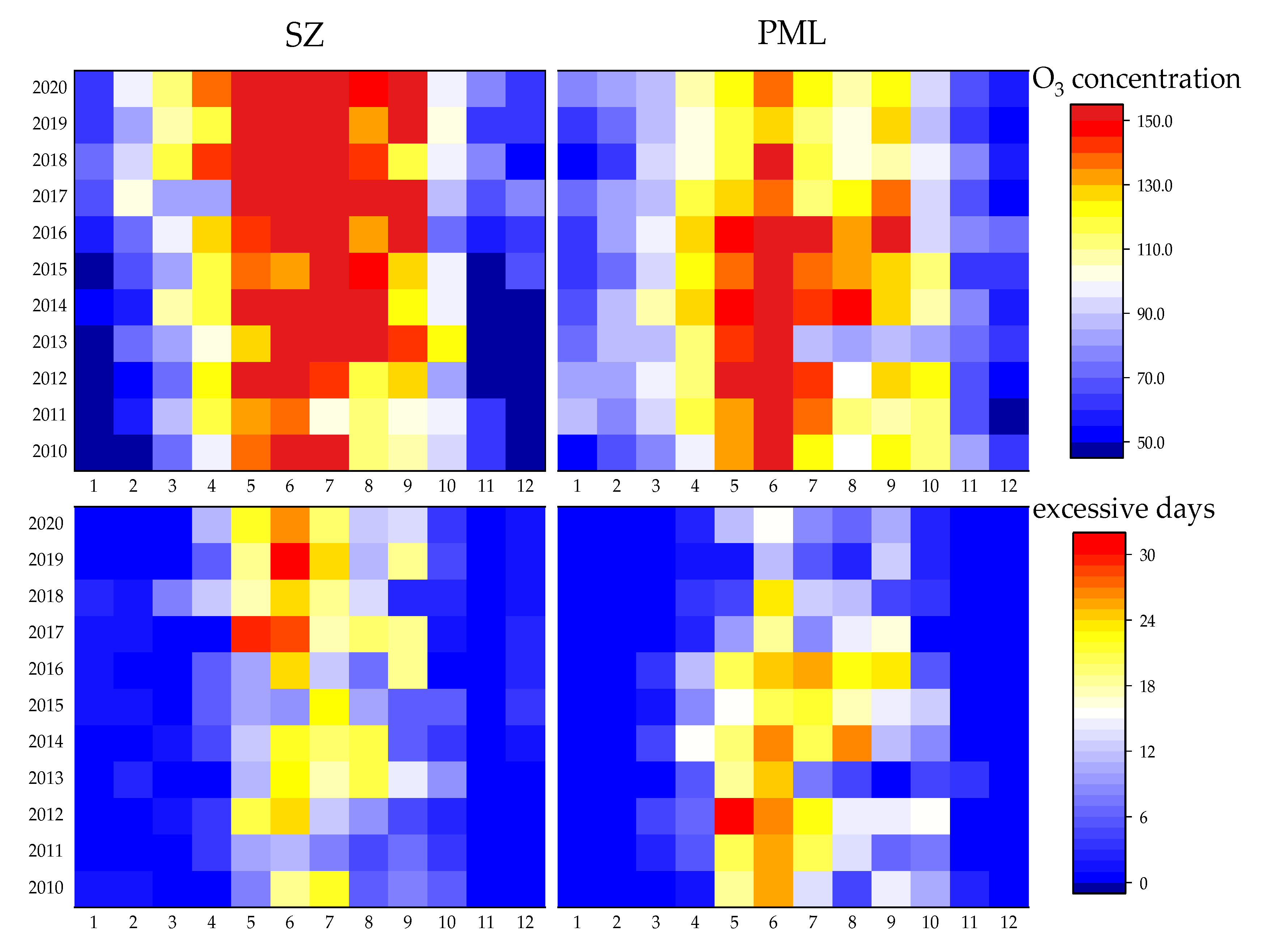
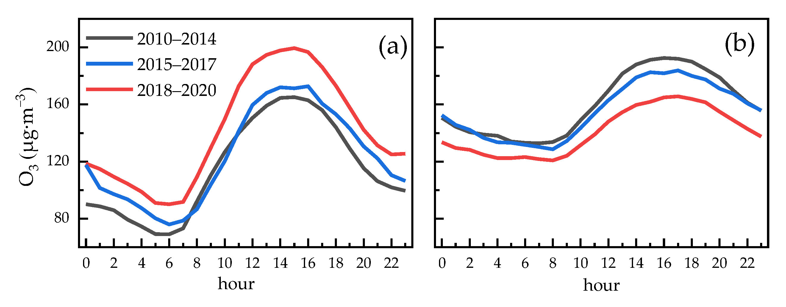
3.1. Temporal Variations of Ozone Concentrations

Figure 2 shows the long-term O3 trend of different percentiles (10th, 50th, and 90th) at the urban (SZ) and suburban sites (PML) in Jinan from 2010 to 2020. As shown in Figure 2, all indicators of surface O3 at SZ show an increasing trend, which indicates an overall increase of O3 in the past decade. This is consistent with other studies at urban sites in China [14,20]. In contrast, the D10th of O3 at PML shows an increasing trend and other indicators show a decreasing trend. This trend of decreasing amplitude is worthy of further study.
D10th represents a low ozone concentration, which generally does not involve or is less involved in the photochemical production of ozone. The change in the D10th O3 value can represent changes in the local background O3 concentration. Thus, the local background O3 of SZ and PML sites increased by about 1.3 μgm−3year−1 and 0.48 μgm−3year−1, respectively, which was lower than that in urban and suburban areas in Beijing, which is located in the north of the NCP [21], indicating a different O3 trend between the central and north areas of the NCP. The different upward trend of D10th O3 at urban and suburban sites may be attributed to the various reduced O3 titrations by NO.
In contrast to the background O3 levels, the changes in the D90th of O3 indicate a change in photochemical ability. There is a faster increase in the daily high concentration of D90th at the SZ site, with an increasing rate of 2.9 μgm−3·year1, which is significantly greater than the increase rate of the D10th. In addition, the D90th of O3 at the PML site presents a significant decreasing trend (2.07 μgm−3year−1), indicating that the photochemical reaction at PML has weakened significantly during the past decade. The entirely different trend of D90th of O3 between the urban and suburban areas suggests the different changes of O3 precursors and meteorological conditions in the two places; both have critical roles in photochemical O3 formation. The annual 90th percentile of the maximum daily 8-h average (90th MDA8), which is commonly used for pollution evaluation, showed serious pollution in both urban and suburban areas, and exceeded the secondary standard limit of 160 μgm−3 from 2010 to 2020, except for certain years in the suburban areas. It is worth noting that the 90th MDA8 O3 also shows different trends in urban and suburban areas, with an increasing trend of 3.01 μgm−3year−1 in urban areas and a sharp decreasing trend of 3.74 μgm−3year−1 in suburban areas. The decreasing trends at the suburban site were also observed at regional sites in Europe, North America, and the PRD region in recent years. In addition, the researchers also found an upward trend for high-value ozone concentrations, increasing in the main urban areas, along with a decreasing trend in the suburban areas in Beijing [21]. This phenomenon suggested that regional photochemical O3 may show a systematical downward trend in the NCP. Furthermore, we found that the annual 90th MDA8 O3 generally fluctuated up and down until 2017; after that time, the high 90th MDA8 O3 showed a continuous downward trend. This observed result indicates that the high O3 levels in the suburban areas of the NCP have reduced in recent years, which shows the likelihood of an overall O3 concentration reduction in the future.
In summary, O3 concentrations in urban areas (SZ) show an overall increasing trend, and the growth rate of the high concentration index is greater than that of the low concentration index, while O3 concentrations in suburban areas (PML) show a slow increase at low values and a rapid decrease at high values. The general rise in low ozone concentrations marks an increase in local ozone background values, but the effect of ozone photochemical production is more important. The increasing ozone pollution in urban areas may be due to the unreasonable control of precursors in urban areas or to adverse meteorological effects. In contrast, the control of high-value ozone was achieved in the suburban areas, probably because the changes of precursors and other factors in the suburban areas affected the photochemical production of ozone and achieved reasonable control of O3, which may have implications for the control of O3 in the whole region.
Figure 3 shows the monthly variations of MDA8 O3 in Jinan from 2010 to 2020. It is obvious that high O3 concentration was concentrated in the “ozone season”, from April to September. Higher temperature and stronger solar radiation indicate stronger photochemical reactions and may produce more O3. The time range of the monthly mean MDA8 O3 at the urban site gradually increased from May–July in 2010 to March–September in 2020. In contrast, the temporal distributions of the high monthly mean MDA8 O3 levels did not change significantly during the decade. In addition, the mean MDA8 O3 in the ozone season was much higher in the urban area than in the suburban area. We also counted the number of days when the O3 concentration was higher than 160 μgm−3, which is defined as the O3 exceedance days with levels over the National Ambient Air Quality Standard (NAAQS) in China. From the long-term perspective, we found that the O3 exceedance days of SZ increased from 63 in 2010 and 42 in 2011 to 109 in 2017 and that the exceedance days maintained higher levels during the following years. Conversely, the O3 exceedance days of O3 in the PML increased to their peak value in 2017, exceeding 133 days, then quickly dropped to 54 days in 2020. The difference in O3 exceedance days also suggests that much stronger summertime photochemical pollution generally occurred in the urban areas.
Both the MDA8 O3 and O3 exceedance days indicate quite different characteristics regarding O3 in urban and suburban areas. However, summer ozone pollution still persisted during the past decade in urban and suburban areas.
From the discussions presented above, it can be seen that high O3 levels generally occurred in June, in both the urban and suburban areas. Thus, we focus on the daily variations of O3 between the urban and suburban areas in three time periods, 2010–2014, 2015–2017, and 2018–2020, respectively.
As shown in Figure 4, the pattern of the diurnal variations did not change substantially in the three periods. The O3 concentration decreased to the lowest level at about 6 a.m. to 7 a.m. and then increased to a peak at about 2 p.m. to 4 p.m. in the urban areas. The peak ozone level occurred one hour later in the suburban areas than in the urban areas, which is consistent with the findings of other researchers [37]. This is mainly due to the delayed transport of precursors from urban to suburban areas [37].
Since ozone precursor emissions are lower at night from 12 a.m. to 4 a.m, when there is no photochemical production, rather than in the daytime, we used the O3 concentrations from 12 a.m. to 4 a.m. as the background O3 concentrations. As can be seen from Figure 4, background O3 concentrations were significantly higher in the suburban areas than in the urban areas; they were increasing in the urban areas and decreasing in the suburbs over the study period.
Another difference in the diurnal variations of O3 between urban and suburban areas is the daily amplitude, which ranges from 60 to 200 μgm−3 at the urban sites and ranges from 120 to 190 μgm−3 at the suburban site. The larger amplitude of O3 concentration in urban areas was mostly because of the stronger photochemical generation of O3 and NO titration. It is worth noting that both the trough and peak values of the diurnal variation of O3 show an upward trend at urban sites, whereas the suburban sites show a downward trend of O3 concentration between 2010 and 2014 and 2018 to 2020. The quite different phenomenon of O3 values indicated that the photochemical formation and depletion of O3 in urban and suburban areas may have an opposite trend.
An interesting finding in this study was the ozone concentrations in urban and suburban areas, which reversed during the three periods, with urban ozone concentrations exceeding those in suburban areas in the 2018–2020 period. The generally accepted notion that ozone concentrations at suburban sites are higher than those at urban sites has been disproved [22,23]. The peak value of O3 diurnal variation at SZ was much lower (~30 μgm−3) than that at the PML site in the 2010–2014 period. However, the difference narrowed to 10 μgm−3 in the 2015–2017 period. The difference flipped in the 2018–2020 period; the peak value at SZ was 35 μgm−3 higher than PML site. In addition, with the decrease of the O3 trough at the suburban site and the increase of the O3 trough at the urban site, the gap between the two gradually narrowed.
In conclusion, O3 concentration in urban and suburban areas presents different characteristics in terms of the long-term trend, high concentration period, and days exceeding the standard and diurnal variations. The relative contributions of the factors influencing the different characteristics of O3 levels in urban and suburban areas will be discussed below.

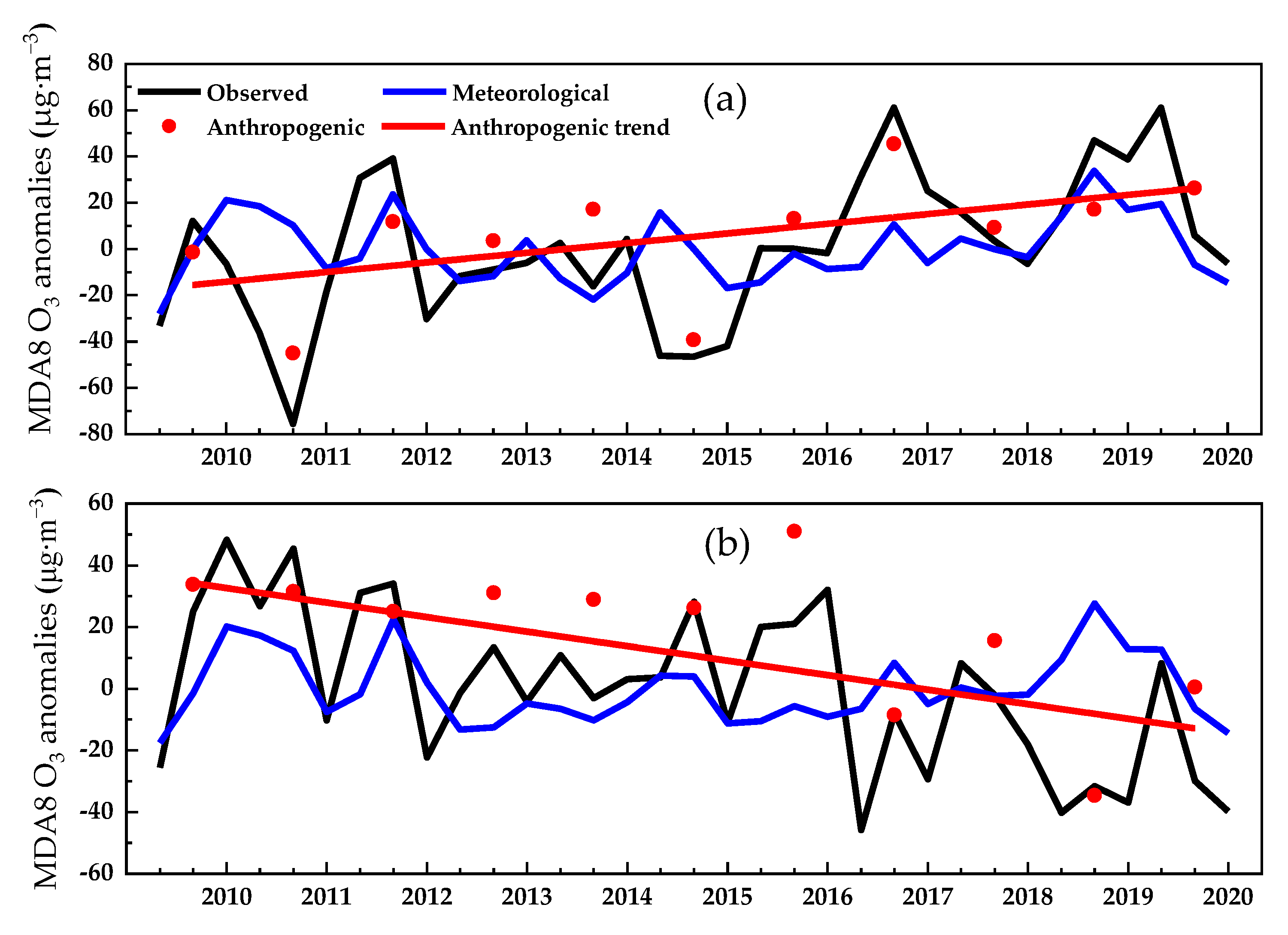
3.2. MLR Modeling and Ozone Contribution Analysis

To quantify the contributions of meteorological and anthropogenic factors to ozone trends, we developed a stepwise MLR model for urban and suburban areas, respectively. The variables selected for urban and suburban areas are shown in Table 3. The coefficients of determination of the MLR models for urban and suburban areas were 0.50 and 0.38, respectively.
Figure 5 shows the meteorologically and anthropogenically driven ozone trends, based on the MLR method; the results are presented in Table 4. We found a meteorologically driven trend of 0.75 μgm−3year−1 for the SZ site and 0.45 μgm−3year−1 for the PML site, which indicates the small positive contribution of meteorological conditions to the MDA8 O3 trend. The predicted contribution of meteorological conditions was 16.2% for the urban site and 8.5% for the suburban site, which are both much lower than the contributions of anthropogenic emissions. We found that the anthropogenic trend of MDA8 O3 was +3.87 μgm−3year−1 for the SZ site, contributing 83.3% of the observed trend. In contrast, the anthropogenic trend of MDA8 O3 was −5.76 μgm−3year−1 for the PML site, contributing about 108.5% of the observed trend. Thus, the MDA8 O3 trends over the 2010–2020 period in the urban and suburban sites received significant contributions from anthropogenic emissions. This is consistent with the results reported by other researchers, who used multiple linear regression models to study the causes of ozone change in the megacity clusters of eastern China [14]. In addition, anthropogenic emissions play opposite roles in the long-term trends of MDA8 O3 in urban and suburban sites, which promoted O3 concentrations in urban areas and reduced ozone levels in suburban areas. Thus, compared with the meteorological conditions, the O3 pollution in Jinan was mostly influenced by anthropogenic emissions.

3.3. Relationship between O3 and Precursors

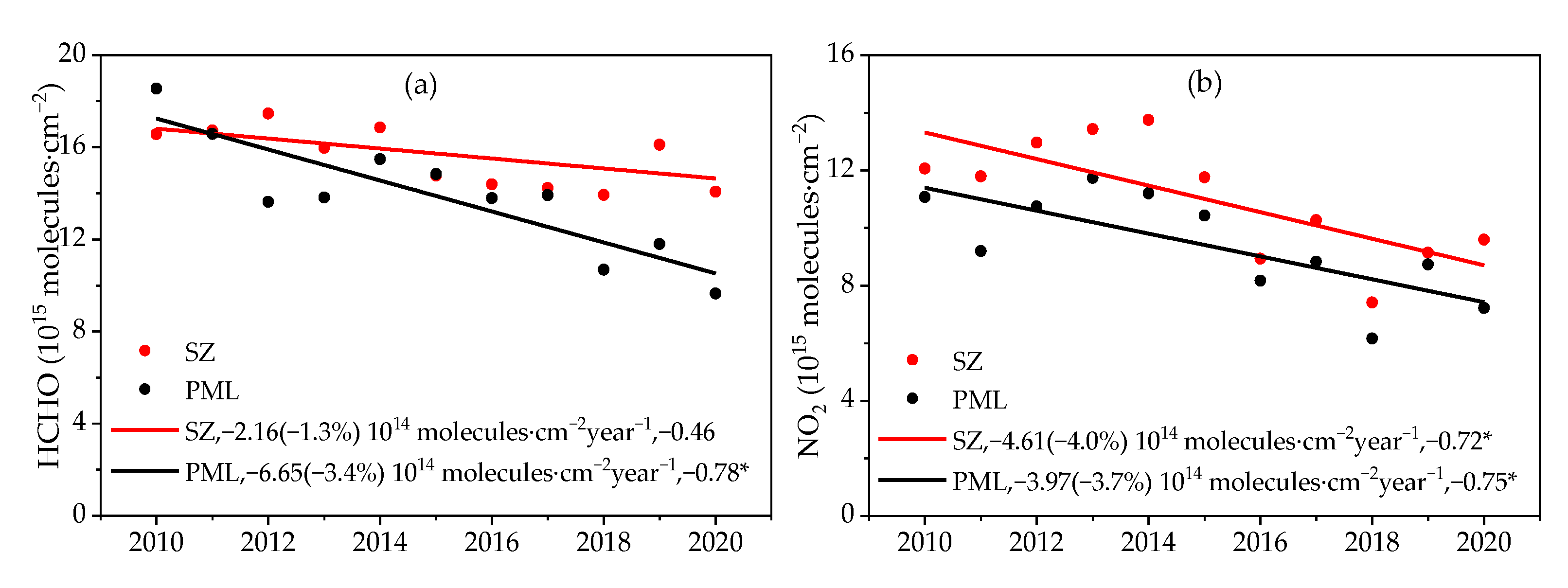
3.3.1. Variations of NO2 and HCHO, as Reported from the Satellite

In consideration of the large contribution of anthropogenic emissions to the long-term O3 trend in Jinan, here, we examine the relationships between the changes in O3 precursor emissions and O3 trends. Due to the wide range of sources of VOCs and the difficulty of data collection, we were unable to obtain 11 years of data for VOCs, since the oxidation of highly reactive VOCs can produce HCHO in the vicinity of the emission source. The HCHO column concentration can be observed by satellite so that the emission rates of VOCs can be inferred. Long-term trends in HCHO column concentrations can largely reflect changes in VOCs concentration. NO2 is the main component of NOX in ambient air; satellite observations of the NO2 trends can largely reflect changes in NOX. The tropospheric HCHO and NO2 column of OMI have been used as the indicators of NMVOCs and NOX emissions [38,39]. HCHO is a short-lived oxidation product of VOCs that is positively correlated with peroxyl radicals and has a direct linear relationship with VOCs [40]. Thus, the accumulation of VOCs can be indirectly reflected by the properties of HCHO [41]. Using the OMI inversion data, Ju et al. analyzed the spatial and temporal distribution and trends of HCHO in Jiangsu, Zhejiang, and Shanghai from 2008 to 2019 and the impact of emissions from various VOCs sources on HCHO [42]. Li et al. found an underestimation of NMVOCs emissions (especially from anthropogenic sources) by improving the emission estimates of reactive NMVOCs in the PRD region for March 2017, based on the HCHO data of OMI [43]. Figures S2 and S3 show that ground-based NOx data have a good correlation and show a similar trend with the satellite NO2 data, which also indicates the availability of satellite data.
The long-term changes in the HCHO and NO2 columns from 2010 to 2020 are shown in Figure 6. The NO2 column decreased by 33%–40% in the urban area at a rate of 4.0% year−1 (p < 0.05). The trend of the NO2 column in the suburban area is similar to that in the urban area, with a decreasing rate of 3.7% year−1. The surface vegetation at the two sites has not changed much in recent years, while the two sites are different pixel points of the satellite data, there is no intermingling phenomenon, which can better reflect the difference between urban and suburban areas. The NO2 data from satellite observations were verified by the trend of NOX changes from the ground observations, and it was found that the decline rate of both ground observations and satellite data during the period was close to about 4% year−1 (Figure S2); the satellite data could better reflect the changes in precursors. Almost the same trend in the NO2 column was seen in the urban and suburban areas, which means that the effective NOX control measures and strategy in Jinan have successfully reduced the emissions of NOX in this region.
However, the effect of VOCs emissions control in the urban and suburban areas was quite different. The trends of the HCHO column in urban and suburban areas were −1.3% year−1 (p > 0.05) and −3.4% year−1 (p < 0.05), respectively. During the observation period, the rate of HCHO decline in suburban areas was slightly lower than that of NO2. In urban areas, the rate of HCHO decline was significantly less than that of NO2, due to the high population density and extensive sources of VOCs, which are more difficult to control. Considering the above-mentioned opposite trend of MDA8 O3 in urban and suburban areas, the different trends of O3 precursor emissions may lead to the change in ozone formation mechanisms over the observed period. The decrease in NOX may promote or inhibit O3 formation, depending on the ratios of the NOX and VOCs levels. Thus, we need to further determine the ozone formation mechanism in both urban and suburban areas.

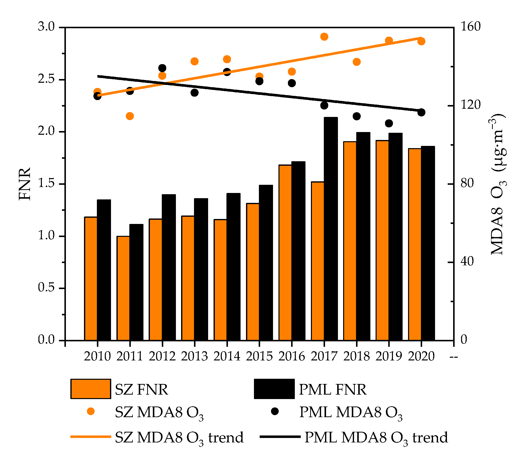
3.3.2. O3–VOCs–NOX Sensitivity

The satellite-based ratio of HCHO to NO2 (FNR) is used as an indicator of the sensitivity of O3 to its precursors, NOX, and VOCs, and is widely used [44,45]. The findings of FNR(HCHO/NO2) < 1.0 and > 2.0 indicate the sensitivity of O3 under VOCs-limited and NOX-limited conditions, respectively, with an FNR of between 1.0 and 2.0 as a transition state. This method was previously used in China to investigate the sensitivity of O3-NOX-VOCs [46].
Figure 7 shows the trend of FNR and MDA8 O3 for suburban (PML) and urban (SZ) areas in the ozone seasons in the period 2010–2020. The FNR values of the urban and suburban areas were generally less than 2.2. For urban areas, the FNR values ranged from 1.2 to 1.9 during the observation period. In comparison, in the suburban areas, the FNR values varied from 1.4 to 2.2. According to the criteria for the ozone formation mechanism described above, ozone production is mostly controlled by both NOX and VOCs emissions, demonstrating a transitional control mechanism. In addition, the FNR values in suburban areas were mostly higher than those in urban areas. This indicates that O3 generation was more affected by NOX emissions in suburban areas than in urban areas, although this phenomenon is not obvious, due to the proximity of the two sites. The FNR showed a significant increase in both urban and suburban areas during the study period, reflecting the different control effectiveness for VOCs and NOX. The NOX emissions of the power plant, factories, and vehicles in urban areas have been vigorously controlled since 2013 in Jinan, but the VOCs emissions have not been controlled as efficiently, which leads to the weakening of NO titration and the increase in O3 formation. This reflects the preference of urban O3 in the transition control of VOCs-limited values. Conversely, in the suburban area, the O3 decreased due to the reduced NOX emissions, indicating the preference of suburban O3 in terms of transition control for NOX-limited values. Thus, the MDA8 O3 values at the SZ site exceeded those at the PML site in 2016, when the gap between them tended to expand.
In summary, the control of urban ozone precursors in Jinan has mainly focused on NOX emissions since 2013, which promoted the reduction of photochemical ozone generation in suburban areas, although this did not solve the problem of the increasing urban O3 levels. Since the ozone formation regime in the urban and suburban areas in Jinan belongs to the transition state, the key to solving the O3 pollution problem in Jinan in the future is to select an appropriate reduction ratio of VOCs/NOX. Therefore, a reasonable way to control ozone pollution would be to reduce NOX emissions while increasing the control of VOCs emissions, rather than merely reducing the NOX emissions. Otherwise, there will be a negative impact in the short term resulting in higher ozone concentrations, especially in urban areas.
The vegetation emissions of BVOCs in suburban areas could affect ozone formation, which may cause some uncertainty in this study. However, since the BVOCs emissions were strongly impacted by temperature, this could be regarded as a meteorological factor in ozone trends. The MLR analysis shows that anthropogenic emissions are the major contributors to long-term O3 trends. In addition, suburban areas have more forests and grasslands than urban areas and emit more BVOCs. However, the HCHO column density in urban areas is still higher than that in suburban areas, indicating that anthropogenic NMVOCs play a dominant role in the figures for total NMVOCs. Above all, these BVOCs emissions could not lead to significant changes in ozone trends and the ozone formation regime.

4. Conclusions

The O3 trends in Jinan in the central North China Plain from 2010 to 2020, as demonstrated in this study, show that high O3 levels increase rapidly in urban areas and decrease quickly in suburban areas. The rate of increase by D90th O3 in urban areas was 2.88 μgm−3year−1, and the 90th MDA8 increased by 3.01 μgm−3year−1; in suburban areas, the rate of decrease of D90th was 2.07 μgm−3year−1, and 90th MDA8 decreased by 3.74 μgm−3year−1. The period of O3 pollution at the urban sites gradually increased from May–July in 2010 to March–September in 2020. In contrast, the temporal distributions of the high monthly mean MDA8 O3 levels did not change significantly at the suburban site. A phased study of the daily variation in the periods of heavy O3 pollution revealed that O3 concentrations in urban areas were reversed, compared to suburban areas, during the period from 2010 to 2020. The maximum value of the daily variation of O3 in urban areas was higher than that in suburban areas by about 35 μgm−3 in 2018–2020.
Anthropogenic influences were the main factor causing the different O3 trends in suburban and urban areas, with meteorological influences playing a non-dominant role. The contribution of anthropogenic effects to changes in O3 was 83.6% in urban areas and 108.5% in suburban areas. Meteorological factors contributed to the O3 increase in both urban and suburban areas.
We analyzed the changes in precursors from 2010 to 2020 and found a significant reduction in NOX in urban and suburban areas, but the control of VOCs was clearly not enough, especially for urban areas. Whereas HCHO showed a non-significant decreasing trend of 1.3% year−1 in urban areas and a significant decrease of 3.4% year−1 in suburban areas, NO2 decreased at the close rates of 3.7% year−1 and 4.0% year−1 in suburban and urban areas. O3 sensitivity regarding FNR shows that both urban and suburban areas were in the VOCs–NOX transition control regime. The difference is that urban areas tend to be more VOCs-limited, while suburban areas tend to be more NOX-limited. Thus, the rapid NOX decline produced different effects in urban and suburban areas. In urban areas, this leads to a weaker titration of NO and enhanced O3 formation, while in suburban areas, this weakens the photochemical production of O3.
The resolution of the O3 pollution problem in downtown Jinan in the future depends on choosing a suitable VOCs/NOX reduction ratio. A reasonable approach to control O3 pollution should be to reduce NOX emissions while increasing the control of VOCs, which would otherwise have negative effects in the short term and lead to higher O3 concentrations, especially in urban areas.

Supplementary Materials

The following are available online at https://www.mdpi.com/article/10.3390/atmos13060994/s1, Figure S1: Validation of MERRA-2 data by meteorological data from ground observations in June 2020, Figure S2: Ground-based observations of trends in NOx and CO. Note: * indicates that the requirement of significance was reached (p < 0.05), Figure S3: Validation of ground-observed NOX against satellite NO2.

Author Contributions

Original draft preparation, J.S. and C.W.; reviewing and editing, S.D. and B.W.; reviewing and revision, L.S. and C.Z.; data curation and investigation, G.F., X.S., Z.X. and B.L.; supervision and reviewing, J.Y. All authors have read and agreed to the published version of the manuscript.

Funding

This research was funded by the National Natural Science Foundation of China (41905111, 42105104), Shandong Provincial Natural Science Foundation (ZR2019BD030, ZR2020QD060), Shandong Province Key R & D project (2019GSF109043), Qilu University of Technology Teaching, and the Research Project (2020yb18).

Data Availability Statement

The meteorological data in this study were obtained from MERRA-2. HCHO, and NO2 data were obtained from OMI. The above data can be found at https://giovanni.gsfc.nasa.gov/ (accessed on 30 September 2021).

Conflicts of Interest

The authors declare no conflict of interest.

References

  1. Chaudhary, I.J.; Rathore, D. Effects of ambient and elevated ozone on morphophysiology of cotton (Gossypium hirsutum L.) and its correlation with yield traits. Environ. Technol. Innov. 2022, 25, 102146. [Google Scholar] [CrossRef]
  2. Moura, B.B.; Brunetti, C.; da Silva Engela, M.R.G.; Hoshika, Y.; Paoletti, E.; Ferrini, F. Experimental assessment of ozone risk on ecotypes of the tropical tree Moringa oleifera. Environ. Res. 2021, 201, 111475. [Google Scholar] [CrossRef] [PubMed]
  3. Wang, Y.; Cao, R.; Xu, Z.; Jin, J.; Wang, J.; Yang, T.; Wei, J.; Huang, J.; Li, G. Long-term exposure to ozone and diabetes incidence: A longitudinal cohort study in China. Sci. Total Environ. 2021, 816, 151634. [Google Scholar] [CrossRef] [PubMed]
  4. Zhao, N.; Pinault, L.; Toyib, O.; Vanos, J.; Tjepkema, M.; Cakmak, S. Long-term ozone exposure and mortality from neurological diseases in Canada. Environ. Int. 2021, 157, 106817. [Google Scholar] [CrossRef] [PubMed]
  5. Xu, X.; Lin, W.; Xu, W.; Jin, J.; Wang, Y.; Zhang, G.; Zhang, X.; Ma, Z.; Dong, Y.; Ma, Q. Long-term changes of regional ozone in China: Implications for human health and ecosystem impacts. Elem. Sci. Anthr. 2020, 8, 13. [Google Scholar] [CrossRef] [Green Version]
  6. Atkinson, R. Atmospheric chemistry of VOCs and NOx. Atmos. Environ. 2000, 34, 2063–2101. [Google Scholar] [CrossRef]
  7. Lin, X.; Trainer, M.; Liu, S. On the nonlinearity of the tropospheric ozone production. J. Geophys. Res. Atmos. 1988, 93, 15879–15888. [Google Scholar] [CrossRef] [Green Version]
  8. Ou, J.; Yuan, Z.; Zheng, J.; Huang, Z.; Shao, M.; Li, Z.; Huang, X.; Guo, H.; Louie, P.K. Ambient Ozone Control in a Photochemically Active Region: Short-Term Despiking or Long-Term Attainment? Environ. Sci. Technol. 2016, 50, 5720–5728. [Google Scholar] [CrossRef]
  9. Pusede, S.E.; Steiner, A.L.; Cohen, R.C. Temperature and recent trends in the chemistry of continental surface ozone. Chem. Rev. 2015, 115, 3898–3918. [Google Scholar] [CrossRef]
  10. Shao, M.; Zhang, Y.; Zeng, L.; Tang, X.; Zhang, J.; Zhong, L.; Wang, B. Ground-level ozone in the Pearl River Delta and the roles of VOC and NO(x) in its production. J. Environ. Manage. 2009, 90, 512–518. [Google Scholar] [CrossRef]
  11. Tan, Z.; Hofzumahaus, A.; Lu, K.; Brown, S.S.; Holland, F.; Huey, L.G.; Kiendler-Scharr, A.; Li, X.; Liu, X.; Ma, N.; et al. No Evidence for a Significant Impact of Heterogeneous Chemistry on Radical Concentrations in the North China Plain in Summer 2014. Environ. Sci. Technol. 2020, 54, 5973–5979. [Google Scholar] [CrossRef]
  12. Li, W.J.; Shao, L.Y.; Wang, W.H.; Li, H.; Wang, X.M.; Li, Y.W.; Li, W.J.; Jones, T.; Zhang, D.Z. Air quality improvement in response to intensified control strategies in Beijing during 2013–2019. Sci. Total Environ. 2020, 744, 140776. [Google Scholar] [CrossRef]
  13. Wang, Y.; Gao, W.; Wang, S.; Song, T.; Gong, Z.; Ji, D.; Wang, L.; Liu, Z.; Tang, G.; Huo, Y.; et al. Contrasting trends of PM2.5 and surface-ozone concentrations in China from 2013 to 2017. Natl. Sci. Rev. 2020, 7, 1331–1339. [Google Scholar] [CrossRef] [Green Version]
  14. Li, K.; Jacob, D.J.; Liao, H.; Shen, L.; Zhang, Q.; Bates, K.H. Anthropogenic drivers of 2013-2017 trends in summer surface ozone in China. Proc. Natl. Acad. Sci. USA 2019, 116, 422–427. [Google Scholar] [CrossRef] [Green Version]
  15. Yang, L.; Luo, H.; Yuan, Z.; Zheng, J.; Huang, Z.; Li, C.; Lin, X.; Louie, P.K.K.; Chen, D.; Bian, Y. Quantitative impacts of meteorology and precursor emission changes on the long-term trend of ambient ozone over the Pearl River Delta, China, and implications for ozone control strategy. Atmos. Chem. Phys. 2019, 19, 12901–12916. [Google Scholar] [CrossRef] [Green Version]
  16. Wang, N.; Lyu, X.; Deng, X.; Huang, X.; Jiang, F.; Ding, A. Aggravating O3 pollution due to NOx emission control in eastern China. Sci. Total Environ. 2019, 677, 732–744. [Google Scholar] [CrossRef]
  17. Lu, X.; Zhang, L.; Wang, X.; Gao, M.; Li, K.; Zhang, Y.; Yue, X.; Zhang, Y. Rapid Increases in Warm-Season Surface Ozone and Resulting Health Impact in China Since 2013. Environ. Sci. Technol. Lett. 2020, 7, 240–247. [Google Scholar] [CrossRef]
  18. Wang, W.; Li, X.; Shao, M.; Hu, M.; Zeng, L.; Wu, Y.; Tan, T. The impact of aerosols on photolysis frequencies and ozone production in Beijing during the 4-year period 2012–2015. Atmos. Chem. Phys. 2019, 19, 9413–9429. [Google Scholar] [CrossRef] [Green Version]
  19. Hu, M.; Wang, Y.; Wang, S.; Jiao, M.; Huang, G.; Xia, B. Spatial-temporal heterogeneity of air pollution and its relationship with meteorological factors in the Pearl River Delta, China. Atmos. Environ. 2021, 254, 118415. [Google Scholar] [CrossRef]
  20. Xiang, S.; Liu, J.; Tao, W.; Yi, K.; Xu, J.; Hu, X.; Liu, H.; Wang, Y.; Zhang, Y.; Yang, H.; et al. Control of both PM2.5 and O3 in Beijing-Tianjin-Hebei and the surrounding areas. Atmos. Environ. 2020, 224, 117259. [Google Scholar] [CrossRef]
  21. Ren, J.; Hao, Y.; Simayi, M.; Shi, Y.; Xie, S. Spatiotemporal variation of surface ozone and its causes in Beijing, China since 2014. Atmos. Environ. 2021, 260, 118556. [Google Scholar] [CrossRef]
  22. Zeng, X.; Gao, Y.; Wang, Y.; Ma, M.; Zhang, J.; Sheng, L. Characterizing the distinct modulation of future emissions on summer ozone concentrations between urban and rural areas over China. Sci. Total Environ. 2022, 820, 153324. [Google Scholar] [CrossRef] [PubMed]
  23. Cheng, N.; Li, R.; Xu, C.; Chen, Z.; Chen, D.; Meng, F.; Cheng, B.; Ma, Z.; Zhuang, Y.; He, B.; et al. Ground ozone variations at an urban and a rural station in Beijing from 2006 to 2017: Trend, meteorological influences and formation regimes. J. Clean. Prod. 2019, 235, 11–20. [Google Scholar] [CrossRef]
  24. Wang, T.; Dai, J.; Lam, K.S.; Nan Poon, C.; Brasseur, G.P. Twenty-five years of lower tropospheric ozone observations in tropical East Asia: The influence of emissions and weather patterns. Geophys. Res. Lett. 2019, 46, 11463–11470. [Google Scholar] [CrossRef]
  25. Wang, T.; Xue, L.; Brimblecombe, P.; Lam, Y.F.; Li, L.; Zhang, L. Ozone pollution in China: A review of concentrations, meteorological influences, chemical precursors, and effects. Sci. Total Environ. 2017, 575, 1582–1596. [Google Scholar] [CrossRef]
  26. Chen, X.; Zhong, B.; Huang, F.; Wang, X.; Sarkar, S.; Jia, S.; Deng, X.; Chen, D.; Shao, M. The role of natural factors in constraining long-term tropospheric ozone trends over Southern China. Atmos. Environ. 2020, 220, 117060. [Google Scholar] [CrossRef]
  27. Sun, L.; Xue, L.; Wang, Y.; Li, L.; Lin, J.; Ni, R.; Yan, Y.; Chen, L.; Li, J.; Zhang, Q.; et al. Impacts of meteorology and emissions on summertime surface ozone increases over central eastern China between 2003 and 2015. Atmos. Chem. Phys. 2019, 19, 1455–1469. [Google Scholar] [CrossRef] [Green Version]
  28. Li, K.; Jacob, D.J.; Liao, H.; Zhu, J.; Shah, V.; Shen, L.; Bates, K.H.; Zhang, Q.; Zhai, S. A two-pollutant strategy for improving ozone and particulate air quality in China. Nat. Geosci. 2019, 12, 906–910. [Google Scholar] [CrossRef]
  29. Shao, M.; Wang, W.; Yuan, B.; Parrish, D.D.; Li, X.; Lu, K.; Wu, L.; Wang, X.; Mo, Z.; Yang, S.; et al. Quantifying the role of PM2.5 dropping in variations of ground-level ozone: Inter-comparison between Beijing and Los Angeles. Sci. Total Environ. 2021, 788, 147712. [Google Scholar] [CrossRef]
  30. Xue, L.; Wang, T.; Louie, P.K.; Luk, C.W.; Blake, D.R.; Xu, Z. Increasing external effects negate local efforts to control ozone air pollution: A case study of Hong Kong and implications for other Chinese cities. Environ. Sci. Technol. 2014, 48, 10769–10775. [Google Scholar] [CrossRef] [Green Version]
  31. Chen, S.; Wang, H.; Lu, K.; Zeng, L.; Hu, M.; Zhang, Y. The trend of surface ozone in Beijing from 2013 to 2019: Indications of the persisting strong atmospheric oxidation capacity. Atmos. Environ. 2020, 242, 117801. [Google Scholar] [CrossRef]
  32. Zulkifli, M.F.H.; Hawari, N.S.S.L.; Latif, M.T.; Abd Hamid, H.H.; Mohtar, A.A.A.; Idris, W.M.R.W.; Mustaffa, N.I.H.; Juneng, L. Volatile organic compounds and their contribution to ground-level ozone formation in a tropical urban environment. Chemosphere 2022, 302, 134852. [Google Scholar] [CrossRef]
  33. Lu, X.; Hong, J.; Zhang, L.; Cooper, O.R.; Schultz, M.G.; Xu, X.; Wang, T.; Gao, M.; Zhao, Y.; Zhang, Y. Severe Surface Ozone Pollution in China: A Global Perspective. Environ. Sci. Technol. Lett. 2018, 5, 487–494. [Google Scholar] [CrossRef]
  34. Malley, C.S.; Henze, D.K.; Kuylenstierna, J.C.I.; Vallack, H.W.; Davila, Y.; Anenberg, S.C.; Turner, M.C.; Ashmore, M.R. Updated Global Estimates of Respiratory Mortality in Adults >/=30Years of Age Attributable to Long-Term Ozone Exposure. Environ. Health Perspect. 2017, 125, 087021. [Google Scholar] [CrossRef] [Green Version]
  35. Simon, H.; Reff, A.; Wells, B.; Xing, J.; Frank, N. Ozone trends across the United States over a period of decreasing NOx and VOC emissions. Environ. Sci. Technol. 2015, 49, 186–195. [Google Scholar] [CrossRef] [Green Version]
  36. Gelaro, R.; McCarty, W.; Suarez, M.J.; Todling, R.; Molod, A.; Takacs, L.; Randles, C.; Darmenov, A.; Bosilovich, M.G.; Reichle, R.; et al. The Modern-Era Retrospective Analysis for Research and Applications, Version 2 (MERRA-2). J. Clim. 2017, 30, 5419–5454. [Google Scholar] [CrossRef]
  37. Xu, J.; Zhang, X.; Xu, X.; Zhao, X.; Meng, W.; Pu, W. Measurement of Surface Ozone and its Precursors in Urban and Rural Sites in Beijing. Procedia Earth Planet. Sci. 2011, 2, 255–261. [Google Scholar] [CrossRef] [Green Version]
  38. Shen, L.; Jacob, D.J.; Zhu, L.; Zhang, Q.; Zheng, B.; Sulprizio, M.P.; Li, K.; De Smedt, I.; González Abad, G.; Cao, H. The 2005–2016 trends of formaldehyde columns over China observed by satellites: Increasing anthropogenic emissions of volatile organic compounds and decreasing agricultural fire emissions. Geophys. Res. Lett. 2019, 46, 4468–4475. [Google Scholar] [CrossRef] [Green Version]
  39. Lamsal, L.N.; Krotkov, N.A.; Celarier, E.A.; Swartz, W.H.; Pickering, K.E.; Bucsela, E.J.; Gleason, J.F.; Martin, R.V.; Philip, S.; Irie, H.; et al. Evaluation of OMI operational standard NO2 column retrievals using in situ and surface-based NO2 observations. Atmos. Chem. Phys. 2014, 14, 11587–11609. [Google Scholar] [CrossRef] [Green Version]
  40. Sillman, S. The use of NOy, H2O2, and HNO3 as indicators for ozone-NOx -hydrocarbon sensitivity in urban locations. J. Geophys. Res. Atmos. 1995, 100, 14175–14188. [Google Scholar] [CrossRef]
  41. Zhu, S.; Li, X.; Cheng, T.; Yu, C.; Wang, X.; Miao, J.; Hou, C. Comparative analysis of long-term (2005–2016) spatiotemporal variations in high-level tropospheric formaldehyde (HCHO) in Guangdong and Jiangsu Provinces in China. J. Remote Sens. 2019, 23, 137–154. [Google Scholar] [CrossRef]
  42. Ju, T.; Fan, J.; Liu, X.; Li, Y.; Duan, J.; Huang, R.; Geng, T.; Liang, Z. Spatiotemporal variations and pollution sources of HCHO over Jiangsu-Zhejiang-Shanghai based on OMI. Air Qual. Atmos. Health 2021, 15, 15–30. [Google Scholar] [CrossRef]
  43. Li, J.; Zhang, M.; Tao, J.; Han, X.; Xu, Y. OMI formaldehyde column constrained emissions of reactive volatile organic compounds over the Pearl River Delta region of China. Sci. Total Environ. 2022, 826, 154121. [Google Scholar] [CrossRef] [PubMed]
  44. Jin, X.; Holloway, T. Spatial and temporal variability of ozone sensitivity over China observed from the Ozone Monitoring Instrument. J. Geophys. Res. Atmos. 2015, 120, 7229–7246. [Google Scholar] [CrossRef]
  45. Duncan, B.N.; Yoshida, Y.; Olson, J.R.; Sillman, S.; Martin, R.V.; Lamsal, L.; Hu, Y.; Pickering, K.E.; Retscher, C.; Allen, D.J. Application of OMI observations to a space-based indicator of NOx and VOC controls on surface ozone formation. Atmos. Environ. 2010, 44, 2213–2223. [Google Scholar] [CrossRef] [Green Version]
  46. Tang, G.; Wang, Y.; Li, X.; Ji, D.; Hsu, S.; Gao, X. Spatial-temporal variations in surface ozone in Northern China as observed during 2009–2010 and possible implications for future air quality control strategies. Atmos. Chem. Phys. 2012, 12, 2757–2776. [Google Scholar] [CrossRef] [Green Version]
Figure 1. The geographical location of the two sites. SZ is the urban monitoring site and PML is the suburban site.
Atmosphere 13 00994 g001
Figure 2. Mean values of daily 10th percentile, 50th percentile, and 90th percentile ozone concentrations (abbreviated as D10th, D50th, and D90th) and the trends of 90th percentile MDA8 (90th MDA8) per year in Jinan from 2010 to 2020. Figure (a) shows the urban area (SZ), and Figure (b) shows the suburban area (PML). Solid line: linear fit curve. Inset: Linear trend and Spearman’s order correlation coefficient. Note: * indicates that the requirement of significance was reached (p < 0.05). The 90th MDA8 O3 corresponds to the right axis and the D10th, D50th, and D90th O3 to the left axis.
Atmosphere 13 00994 g002
Figure 3. Monthly variations of MDA8 O3 concentration and O3 exceedance days in Jinan from 2010 to 2020, in urban (SZ) and suburban (PML) areas.
Atmosphere 13 00994 g003
Figure 4. The characteristics of daily ozone variations in June during the period from 2010 to 2020. Figure (a) shows the urban area (SZ), and Figure (b) shows the suburban area (PML).
Atmosphere 13 00994 g004
Figure 5. Time series of the anomalous values of MDA8 O3 and MLR-simulated values (one node every ten days in June). The residuals are plotted for the June mean and describe the impact of human activities on ozone. Figure (a) shows the urban area (SZ), and Figure (b) shows the suburban area (PML). The black and blue lines represent the time series of the observed and meteorological predictions of ozone anomalies, respectively. The red dots are the mean values of the residuals between the observed and modeled values, representing the anthropogenic influence of ozone. The red line is a fitted line to the red dots, representing the trend in ozone fluctuations due to the anthropogenic influence.
Atmosphere 13 00994 g005
Figure 6. Trends in HCHO and NO2 from the satellite observations in June for the period 2010–2020. Urban (SZ) and suburban (PML). Solid lines: linear fit curves. Inset: Annual linear trends in parentheses are the percentage rates and Spearman’s order correlation coefficients. Note: * indicates that the requirement of significance was reached (p < 0.05). Figure (a) shows HCHO and Figure (b) shows NO2.
Atmosphere 13 00994 g006
Figure 7. Changes in FNR (HCHO to NO2 ratio) and ozone MDA8 in urban (SZ) and suburban (PML) areas in April–September from 2010 to 2020.
Atmosphere 13 00994 g007
Table 1. Description of the ozone metrics used in this study.
MetricDefinitionAggregation Period
MDA8 (μgm−3)Daily maximum 8-h averageDaily
90th MDA8 (μgm−3)90th percentile of MDA8Annual
D10th, D50th, D90th (μgm−3)Daily 10th, 50th, and 90th percentile 1-h ozone levelsDaily
Table 2. Air quality standards used in China (GB 3095-2012).
PollutantAverage TimeSecondary Standardized Limit ValueUnit
O31-h average200μgm−3
Daily maximum 8-h average160μgm−3
Table 3. Meteorological variables that are considered ozone covariates.
Variable NameDescription
Tmax 1,2Daily maximum 2-m air temperature (K)
U1010-m zonal wind (m s−1)
V10 110-m meridional wind (m s−1)
TCCTotal cloud area fraction (%)
Rainfall 1Precipitation (mm d−1)
SLPSea level pressure (Pa)
RH 1,2Surface air relative humidity (%)
SF 2surface incident shortwave flux (clear sky) (W m−2)
WS 2surface wind speed (m s−1)
The variable chosen for the urban area is 1 and for the suburban area, it is 2.
Table 4. Contribution of meteorological and anthropogenic factors to ozone pollution.
Trend (μgm−3year−1)Contribution (μgm−3)Ratio (%)
SZObserved4.62 *50.82
Meteorological0.758.2516.2 (%)
Anthropogenic3.87 *42.5783.8 (%)
PMLObserved−5.31 *−45.54
Meteorological0.454.73+8.5 (%)
Anthropogenic−5.76 *−50.27−108.5 (%)
Note: * indicates that the requirement of significance was reached (p < 0.05).
Publisher’s Note: MDPI stays neutral with regard to jurisdictional claims in published maps and institutional affiliations.

