1. Introduction
As a chaotic system, the weather prediction models, which suffer from uncertainty in initial conditions and parameters, are very sensitive to its initial conditions [
1]. With small errors in initial conditions, even the short-term state variables result in a big gap between forecasting and truth. Besides, the impact of small-scale processes on large-scale processes must be parameterized in practice due to the limitation of computational recourses [
2,
3]. Though some of the parameters have definite physical meaning in NWP systems and can be deduced from observations empirically or based on physical laws, there are lots of underlying parameters which cannot be easily inferred from observations [
4]. For long-term predictions, the parameterizations influence the behavior much more than in short-term forecasting [
5].
An effective mean to alleviate the uncertainty of initial conditions and parameters is using the information extracted from realistic observations. Data assimilation algorithms, such as variational methods [
6,
7] and ensemble Kalman filter methods (EnKF) [
8], are proposed to involve the information from observations into state variables. Under similar statistical assumptions that the error is multi-dimensional Gaussian distributed, variational data assimilation schemes and EnKF data assimilation schemes are similar [
9]. Constructing covariances to describe the evolution of errors is the key to both variational methods and EnKF methods.
The variational data assimilation methods use a static and flow-independent background error covariance. Various studies developed spatially inhomogeneous and anisotropic background error covariance [
10,
11,
12,
13,
14,
15]. As a non-sequential data assimilation scheme, if not combined with a specific estimation method, like the method proposed by the National Meteorological Centre (NMC) [
16], and re-estimated with the covariance at the beginning of a data assimilation cycle, four-dimensional variational (4DVar) data assimilation scheme itself cannot provide an explicit flow-dependent error covariance at the next cycle window. By the great superiority of assimilating all observations spread over a data assimilation window simultaneously and taking the model constraint into account, 4DVar has been widely used in operational systems [
17]. However, the cost of this advantage is high. Coding and maintaining the tangent linear model and adjoint model of a specific operational system often costs many human resources but cannot be easily transplanted to other models.
In contrast to variational methods, EnKF uses the flow-dependent covariance explicitly. Improved from Kalman filter theory and extended Kalman filter (EKF) [
18], EnKF estimates the error covariance by ensemble members. Once the observation is introduced, the algorithm updates the forecast states straightforwardly. In these loops, the initial conditions are not updated so that the adjoint model is avoided [
19]. Hence, EnKF and its varieties [
20,
21] have been also widely used recently.
Although the variational methods and EnKF achieve similar performances in NWP models, both of them have merits and demerits [
22,
23]. As many studies mentioned, an attractive issue is to combine both sides to improve performance. A typical development is introducing ensemble-based covariance into the variational framework to make the background error covariance is flow-dependent [
24,
25,
26,
27]. When combined with 4DVar, since the integrations of the tangent linear model and adjoint model are also necessary, these kinds of algorithms are named as ensemble four-dimensional variational methods (En4DVar) [
28]. The second typical development, so-called four-dimensional ensemble variational method (4DEnVar), goes even further. Introduced by Liu et al. [
29], the 4DEnVar algorithm not only introduces ensemble-based covariance but also avoids the use of tangent linear model and the adjoint model. In their studies, experiments based on the one-dimensional shallow water model were conducted to prove its efficiency. Initially, Liu et al. [
29] called the proposed 4DEnVar as En4DVar method. With the continuous emergence of hybrid method, Lorenc et al. [
28] renamed it as 4DEnVar method at the World Meteorological Organization (WMO) meeting to highlight its essence as a variational method without adjoint models.
Because of the good properties of 4DEnVar mentioned above, this method has attracted much attention and developed rapidly in theory and application. The POD-E4DVar method proposed by Tian et al. [
30] uses the POD method (proper orthogonal decomposition) to decompose the set members into orthogonal state variables and represents the analysis field as a linear combination of these orthogonal state variables, which effectively avoids the use of adjoint mode. Although, in the study of Tian et al. [
30], POD-E4DVar relies on 4DVar framework, this method is still enlightening and pioneering. Liu et al. [
31] proposed an applicable localization scheme to apply this method to operational analysis and prediction. In 2013, Liu and Xiao [
32] used 4DEnVar to assimilate data from radiosonde ships to study a cyclone process in the Ross Sea in the South Pacific. Buehner et al. [
25] compared the assimilation effects of 3DVar, 4DVar, EnKF, and 4DEnVar. Lorenc et al. [
33] combined the flow dependent background error covariance matrix estimated by the ensemble members with the static background error covariance matrix constructed by the climate state in the Met Office operational system, proposed the hybrid 4DEnVar and compared it with En4DVar. Goodliff et al. [
34] used Lorenz-63 model to compare the differences of assimilation algorithms including 4DEnVar under different observation frequencies and different assimilation window lengths. Tian et al. [
35] and Zhang and Tian [
36] proposed a series of nonlinear least squares En4DVar (NLS- En4DVar) and carried out experimental verification based on Lorenz-96 model. Although named as En4DVar, it is in fact a 4DEnVar method that takes the analysis field as the linear combination of orthogonal state variables. Tian et al. [
37,
38] further constructed ensemble members from historical data and improved the performance of existing algorithms by introducing constraints in the cost function [
39] and improving its optimization iterations.
In another paper [
40], the 4DEnVar proposed by Liu et al. [
29] was improved by our team to capture the model nonlinearity. A new adjoint free data assimilation method called the analytical four-dimensional ensemble variational data assimilation method (A-4DEnVar) was proposed. As mentioned above, the 4DEnVar is motivated by containing the flow-dependent information into background error covariance and also avoids using the adjoint model in data assimilation. However, if the ensemble perturbations are not small enough, the gradients 4DEnVar provided are not the same as that from 4DVar (even they use the same background error covariance and cost function) under strong nonlinear situations. This is mainly because 4DEnVar maintains the idea of EnKF, in which the covariance of the ensemble members is the same as background or analysis error covariance. As the ensemble members are not close enough to the prior estimation, the high order terms in the Taylor expansion influence the estimation accuracy of the adjoint model (see
Section 2 below for more details). Thus, the gradients are not well calculated in 4DEnVar. To better obtain the adjoint model and gradients, the high order terms in Taylor expansion should be as small as possible. To this end, A-4DEnVar constructs the covariance of ensemble members by multiplying the background covariance by a small factor (denoted as
in our formula derivation). Furthermore, to keep consistent with 4DVar, the ensemble perturbations in A-4DEnVar are calculated through centralizing the ensemble members to the evolution of a prior field rather than the mean of these ensemble members as 4DEnVar does. In addition, it is well known that the value of the adjoint model is updated iteratively in 4DVar to capture the nonlinearity. A similar update of the prior initial states in A-4DEnVar is also included to achieve the same effect. We also notice that some variants of 4DEnVar, like NLS-En4DVar [
36], also introduced an iterative loop to greatly improved its processing ability of nonlinearity. With these improvements, the A-4DEnVar completely inherits the properties of the conventional 4DVar scheme. Especially, the background error covariance used in A-4DEnVar and 4DVar could be the same. The covariance is not flow-dependent at the beginning of the first data assimilation window. However, if the data assimilation is proceeded in many cycle windows, i.e., the end of one window is the beginning of the next, it is also possible to construct a flow-dependent covariance in A-4DEnVar as 4DEnVar does. This issue will be discussed in our future work.
Many studies focused on optimizing the initial conditions using 4DEnVar algorithms. Following the development of its theory, Liu et al. [
31,
32] incorporated 4DEnVar into the Advanced Research Weather Research and Forecasting (ARW-WRF) model. Buehner et al. [
25] and Lorenc et al. [
33] compared these hybrid variational and ensemble methods in global NWP systems. Liu et al. [
41] also discussed the relationships of several 4DEnVar algorithms. Liu et al. [
42] used a developed 4DEnVar algorithm, i.e., dimension-reduced projection four-dimensional variational data assimilation scheme (DRP-4DVar), to optimize initial conditions in the Lorenz-96 [
43] model. In Liang et al. [
40], we optimized initial conditions in the Lorenz-63 model. However, as mentioned above, beyond the initial conditions, the state-of-the-art NWP systems consist of uncertainty caused by parameterizations as well. It is widely acknowledged that the conventional data assimilation methods also provide efficient ways to solve the combined state and parameter estimation problem. There are many such studies. To name a few, see [
44,
45] for 4DVar and see [
46,
47,
48,
49,
50] for EnKF.
It is illustrated that the A-4DEnVar works as well as conventional 4DVar, even with a small ensemble size and a relatively long data assimilation window with sparse observations. However, the joint–estimation problem has not been well discussed in A-4DEnVar. It is expected to incorporate the simultaneous estimation method under the framework of A-4DEnVar. Therefore, this issue is to be addressed in the paper. In this paper, we developed A-4DEnVar to estimate the initial conditions and parameters simultaneously. At the beginning of the paper, we consider the evaluations of both state variables and parameter perturbations in the dynamic model. The adjoint models are related to the temporal-spatial covariances of these perturbations. After introducing an approximation of the true initial conditions, the analytical solution of the minimizations of cost function is represented using adjoint models. Then, replacing the adjoint models with temporal-spatial covariances, the adjoint models can be removed. Experiments are conducted to show the equivalence of proposed A-4DEnVar with conventional 4DVar in the joint estimation problem.
This paper is organized as follows.
Section 2 shows the proposed estimation algorithm and its derivation.
Section 3 validates the performance of the A-4DEnVar by the Lorenz model with three parameters. Summary and conclusions are given in
Section 4.
2. Methodology
2.1. Relating the Adjoint Models to Second-Order Statistics
Suppose that the dynamic system is defined as
where
denotes the model operator evolves from time
to time
, and
,
and
are the state variables, model parameters, and forcing terms, respectively. To begin the data assimilation, we assume that the prior estimations of the initial condition and parameters are known and denoted as
and
, respectively. Using the same dynamic model in the equations above, under a strong constraint framework, the estimation satisfies
Suppose any other approximation of
is composed of the a priori estimation and a perturbation (here, marked with a tilde), i.e.,
In contrast to our earlier study, the parameters are also included in the combined estimation problem. Substituting these equations into the dynamical model and expressing through Taylor series expansion gives
where
and
represent the tangent linear expansion of the dynamic model
with respect to the state variables and parameters, respectively. We do not optimize the forcing terms in this paper, so that the tangent linear model about the forcing terms is omitted without any misunderstanding. Comparing Equation (4) with Equation (2) leads to a one-step evolution of the perturbations based on the tangent linear model, i.e.,
We emphasize here that, although Equation (5) was also mentioned in previous studies like Liu et al. [
29], it is often overlooked that the perturbations must be particularly small. The background error covariances are usually too large to be used directly, so without any modification they are not a reasonable choice for
or
. It is easy to generalize the result to the multiple steps evolution corresponding to the initial perturbations
where
represents the tangent linear model from time step
to time step
, and
demonstrates the compound tangent linear models with respect to state variables and parameters. Note that the above derivations hold for any perturbations that are small enough so that the high order terms in Taylor expansion can be neglected. Different from conventional 4DEnVar and EnKF schemes, the perturbations in A-4DEnVar are used to estimate the adjoint models as shown below.
If there are
perturbations
substituting them into Equation (6) yields
Multiplying
by both sides of the equation, it yields
Again, multiplying
by both sides of the equation, it yields
If the ensemble size is large enough, the estimation of the tangent linear model is obtained through
where
is the transpose operator. In the above equations, the distributions of perturbations are not determined or fixed yet. It is easy to see that Equations (11) and (12) holds for any small perturbations and these perturbations do not have to be (though they could be) flow-dependent. In other words, the structure of the adjoint model can be determined by a specially designed Monte Carlo method. A probability density that ignores the interactions between the perturbations of state variable initial conditions and that of parameters is acceptable. With the probability density, the estimations can be simplified as
The tangent linear model here is related through the temporal cross covariances and , the error covariance of ensemble initial condition , and the error covariance of the ensemble parameters for any time step , i.e., and . Especially, describes how the initial conditions are related to parameters. Symbols and are the transposes of and , that are and .
In the derivations above, the tangent linear models and their adjoint models are connected to the second-order statistics of perturbations. Therefore, it is possible to replace adjoint models with these statistics of ensemble members. Besides, the temporal cross covariances are involved in the analytical solution of the cost function in the next subsection to further simplify the calculation. The equations mentioned above hold for any time step , but the temporal covariances are only necessary at the time where observations exist (see more details in the next subsection).
2.2. Expressing Analytical Solutions Using Temporal Cross Covariances
In conventional 4DVar schemes, the cost function is defined as
in which
is the background initial condition,
denotes the parameters in the dynamic model as mentioned in the above subsection, and
are the state variables at time
. Here,
,
and
are the observation mapping operator, observations, and the error covariance of observations, respectively. The background regularization term for parameters is not included in the cost function above because it is difficult to be well determined in reality. Hence, parameters are estimated only based on the observational information in this paper.
Note that although the observation mapping operator might be nonlinear, it can be linearized as
by using similar processes discussed in
Section 2.1. Considering Equations (1)–(3) and (6), the cost function concerning perturbations is
where
is the observational innovation at time step
. In Equation (16) and henceforth, parts of subscripts of adjoint models are omitted to simplify notations. The gradient of the cost function concerning
and
were then calculated using
In conventional 4DVar, numerical optimization algorithms such as gradient descend methods are often used. In contrast to the conventional 4DVar, we solve the equations above directly to achieve its analytical solutions. To further simplify the descriptions, we introduce notations below
to denote the summation terms. Here,
and
represent the tangent linear model
and/or
, or the temporal cross covariance
and/or
. Thus, the minimum solution of the cost function is (See more details in
Appendix A for the derivations)
Or eliminating the adjoint models, the equations are equivalent to
To ensure that the generated perturbations are small enough, we generate ensemble members using
where
is a small factor to ensure the high order terms in Taylor expansion could be omitted. In practice, with cycled data assimilation, the perturbations could not always satisfy small perturbations in all windows, especially with nonlinear regimes. Once the perturbations are too large, the ensembles should be regenerated. Theoretically, the value of factor
is related to the spectral norms of the Hessian matrix of dynamic models and should be carefully determined. However, it is difficult to calculate the spectral norms. An efficient way is set the factor to be as small as possible, and empirically, setting
to be less than 10
−6 is often acceptable. Here, the specially designed construction of
also makes it possible to introduce a flow-dependent covariance estimation method (see next subsections for details). Assuming that the parameters to be estimated are mutually independent,
is a diagonal matrix with its non-zero elements being the ensemble error variances of the parameters and
is the number of parameters. Then, Equations (22) and (23) leads to
Equations (24) and (25) shows that the information introduced into the increments are composed of three parts, i.e., the difference between the background initial conditions with the prior approximation
, observational innovations transmitted through the state variables
and through parameters
. The solution of the cost function is analytical for fixed approximations
and
. We call the proposed method analytical 4DEnVar to be consistent with Liang et al. [
40]. However, the form of solution is much more complex than what we obtained in the earlier study because the interactions of initial conditions and parameters were included.
It is interesting to note that the increments of state variables and parameters are similar except for the term
which is related to the background term in the cost function. In fact, the parameters are regarded as special time-invariant state variables. This treatment process is similar to previous studies of Koyama and Watanabe [
51]. In their study, the so-called state augmentation method regards time-varying parameters as state variables. The estimation processes of state variables and parameters are separated from each other. State variables are assimilated in several cycle windows by conventional EnKF firstly, then the parameters are estimated using the imperfect analysis state variables. In contrast to it, the estimation of state variables and parameters proceeded at the same time under the framework of A-4DEnVar in our study.
When considering the single estimation problem for initial conditions or parameters, it is a natural step to assume the parameters (or initial conditions) are accurate. The corresponding perturbation increment reduces to
The algorithm proposed is in fact equivalent to the Newton iteration method used in conventional 4DVar [
40]. As is well known that the Newton iteration is sensitive to the initial conditions, to make the algorithm stable, a linear search process is necessary. When updating analysis state variables, we add the weighted perturbation
to
, and
and
are the weights minimizing the cost function under the increment direction
. After the linear search,
is updated and then substituted into the next iteration to regenerate ensemble members and calculate a new increment. The process is finished when the difference of the value of the cost function between two iterations is less than tolerance.
While in real atmospheric and oceanic models, the dimension of state variables is huge, the terms with inverse are difficult to calculate. To overcome the obstruction, A-4DEnVar methods estimate the corresponding pseudo inverses instead of the inverse matrix itself by using a few ensemble members. Since the ensemble size is not very large, if we denote the ensemble perturbations as
where is the ensemble size, its pseudo-inverse is . Note that is an matrix, then could be easily calculated. Besides, any inverse term in Equations (24) and (25) and/or Equations (26) and (27) can be decomposed as , where is a symmetric matrix with rows and columns. Based on the decomposition, one can easily calculate the value of and . We emphasize that a compatible localization approach is also necessary for this situation (see more details in next subsections). However, as a proof of concept, under the simplified models whose degree of freedom is small, like the Lorenz model we used below, the inverses are directly used in this paper.
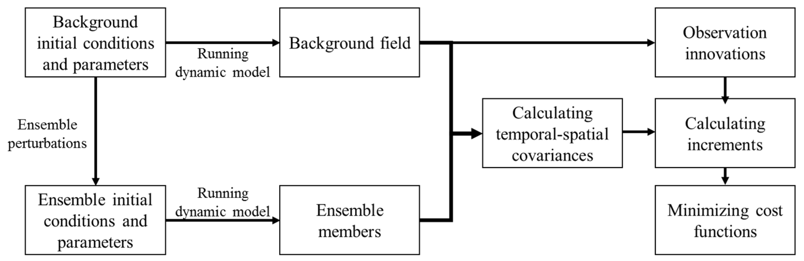
The flowchart of A-4DEnVar method is shown below (
Figure 1).
2.3. Flow-Dependent Covariance and Localization Method
The proposed A-4DEnVar is not a traditional hybrid scheme. The advantage of A-4DEnVar is that the adjoint model is avoided. Although the ensembles in A-4DEnVar are mainly used to estimate the adjoint model, the uncertainty of state variables and parameters are also propagated through these ensembles. It is also possible to propose a flow-dependent scheme in A-4DEnVar.
If an initial condition
is the center of ensemble initial condition, i.e.,
where
denotes the initial condition of ensemble members and
is a zero-mean random noise. In 4DEnVar,
denotes the true initial condition and is unknown. However, in A-4DEnVar,
denotes the background or the prior initial condition. It is known exactly and is updated in each iteration.
It is easy to calculate
and
. Here
and
are the expectation and variance operator, respectively. After integration through a dynamic model, say
, for example, one would obtain the ensemble state variables at time
,
Hence, the uncertainty of the state variables is
Here,
is the tangent linear model. However, because the true state is unknown yet, 4DEnVar replaces
with
, which is only acceptable under a linear or weakly nonlinear situation. In A-4DEnVar, the uncertainty (which is related to the initial state
) is calculated directly without any approximation. In addition, a factor is multiplied bythe perturbation in A-4DEnVar, but its influence can be easily removed by dividing the perturbations by the square of the same factor when estimating the variance, i.e.,
To better consider the flow-dependent error covariance, a combination of traditional 4DEnVar and A-4DEnVar is also useful. However, such issues are beyond this paper. A more detailed discussion combined with localization methods will be addressed in our future work.
It is well known that the dimensions of state variables in real operational system are often huge. The huge dimension usually introduces unexpected problems. One of them is how to localize the background error covariance so that the long-distance pseudo correlations between state variables introduced from a finite of ensemble members are eliminated. Although this paper focuses on the derivation of the algorithm, here we also present a convenient improvement of A-4DEnVar to implement localization. Motivated by Liu et al. (2009), the localization of background error covariance is proposed through extended ensemble members. The process is briefly described below.
In A-4DEnVar, the set of ensemble perturbations is an
-column matrix
,
where
is the ensemble size, and the
th ensemble perturbation
is a column vector. The background error covariance without localization is
Generally, to localize
one often modifies it by a correlation function, such as the Schur operator for example. The localized background error covariance is defined as
and
denotes the spatial correlation function. Suppose
is decomposed as
in which
is a matrix composed of
empirical orthogonal functions of
. It is demonstrated in Liu et al. [
28] that the localized error covariance is
where
and
is an
-column matrix with its every column
.
It is easy to see that the construction of localized background error covariance is similar with itself but with more ensemble members. If the extended ensemble size is also not very large, the solution of A-4DEnVar algorithm (Equations (24) and (25)) is not changed, even with localization in practice.
3. Experiments and Results
3.1. Twin Experiment Setup
Before being performed in operational systems, it is important to study the method in some simple but widely accepted models to test the method. Since this is the first step of our study, a highly nonlinear chaotic ideal model is used here. More complicated models will be studied in the future. In this subsection, we follow the study of Miller et al. [
52], Kalnay et al. [
22], and Goodliff et al. [
34], and use the Lorenz [
1] model (Lorenz-63, henceforth) for verification of A-4DEnVar data assimilation. Although the Lorenz-63 model consists of only three variables and three parameters, it is a strong nonlinear model. The six degrees of freedom make it possible to carry out experiments with full rank. The governing equations of the Lorenz-63 model are
where
is the Prandtl number,
a non-dimensional wave number, and
a normalized Rayleigh number. The standard and default values of parameters are set to be
which were widely used in previous studies. The model runs for truth solutions using a fourth-order Runge-Kutta numerical scheme with time step
and starting from the same initial condition as in Goodliff et al. [
34], i.e., (−3.12346395; −3.12529803; 20.69823159), which were obtained after disregarding the first 1000 steps of an integrating process.
For the experiments constructed in this paper, all three model state variables are observed. The simulated observations are sampled from the truth model state variables contaminated by Gaussian noise with its mean zero and variance 1.0 at regular periods. The background initial conditions were obtained by adding Gaussian noise with covariance
to the initial truth. Considering the interactions between variables, the background error covariance is provided by a three-dimensional variational data assimilation (3DVar) process with a 5000 time-step cycle. The cycle includes many end-to-end assimilation windows and only one observation at the end of each window. Starting from an arbitrary symmetric
and initial conditions, the 3DVar provides an analysis state in a data assimilation window. Then, integrating the analysis state, one would obtain a forecast state
in the next window. The truth states
in the next window can also be calculated easily through integrating the truth initial conditions. Repeat the assimilation and forecast processes until the end of the cycle. A new
is estimated as
from
to
. Again, repeat the estimations. The
usually converges to
in less than 10 iterations.
The determination of parameters is even more complicated than that of initial conditions. There are two empirical strategies to get the parameters. The first demonstrates that no prior information about the parameters is known so that the variance of three parameters might be the same for convenient. The second multiplies a factor by the value of the parameters as their variances. It is hard to point out which is better. However, the main purpose of this paper is to propose the A-4DEnVar for joint estimation problems and show its consistency with conventional 4DVar. Therefore, the two strategies are both acceptable here. In this paper, the initial parameters are calculated by adding random noise with variance 0.25 to the default parameters. Besides, we also conducted experiments based on the variance considered the difference of the parameters, i.e., the variances are set to be , which is one percent of their values. Obviously, the variances are much less or slightly larger than what is used below. Experiment results also demonstrate that A-4DEnVar performs as well as conventional 4DVar. However, we do not show these results in this paper for the limitation of spaces.
To estimate the adjoint models through temporal cross covariances, we add Gaussian noise with covariance (in all experiments, we set ) to the initial conditions and another white noise with variance to the background parameters to generate ensemble members. In this paper, these noises are regenerated in every iteration to be consistent with the derivations. To reduce computational cost, it is not always necessary to update them in practice if ensembles are close enough to . In future works, more efficient generation methods will be discussed, but it is beyond the scope of this paper.
The widely used root-mean-square error (
) as a criterion to appraise the performance of A-4DEnVar and conventional 4DVar schemes. Here, the RMSE for the variable
is defined as
where
represents the number of time steps contained in all time windows (or cycles) in an experiment,
is the analysis state variable and
is the true state variable at time step
. The
mentioned below is calculated from all variables,
where
is the degree of freedom and it is three for both state variables and parameters in the Lorenz-63 model.
3.2. Comparison with Conventional 4DVar
In this subsection, we compare the performance of A-4DEnVar with conventional 4DVar. The experiment settings for window length, observational period, ensemble size, etc., are as follows.
A long data assimilation window may introduce multiple minimums for the cost function. For the single initial condition estimation problem, Kalnay et al. [
22] recommended that the optimal window length when observed every 8 time steps is about 32 time steps, and if observed every 25 steps the optimal window length is from 50 to 125 steps. However, as it is known that the simultaneous estimation for initial conditions and parameters is much more complex than the single estimation problems, it is reasonable to use a data assimilation window that is shorter but can also touch the ultimate window length of 4DVar. Thus, we choose 72 steps for a compromise. Besides, we set the observational period to be 12 time steps in the preliminary test. We conducted experiments with an observational period of 24. However, due to the nonlinearity of the chaotic system, it is very hard for both 4DVar and A-4DEnVar to achieve stable performance. For some initial conditions or parameters, algorithms converge to local minimizers that are far away from the truth, which indicates the failure of data assimilation. Therefore, we do not show these results in this paper. The experiment is designed as end-to-end cycles with 14,400 time steps, i.e., 200 windows. One must note that it may be possible to produce special optimal methods to extend the length of assimilation windows and observation periods.
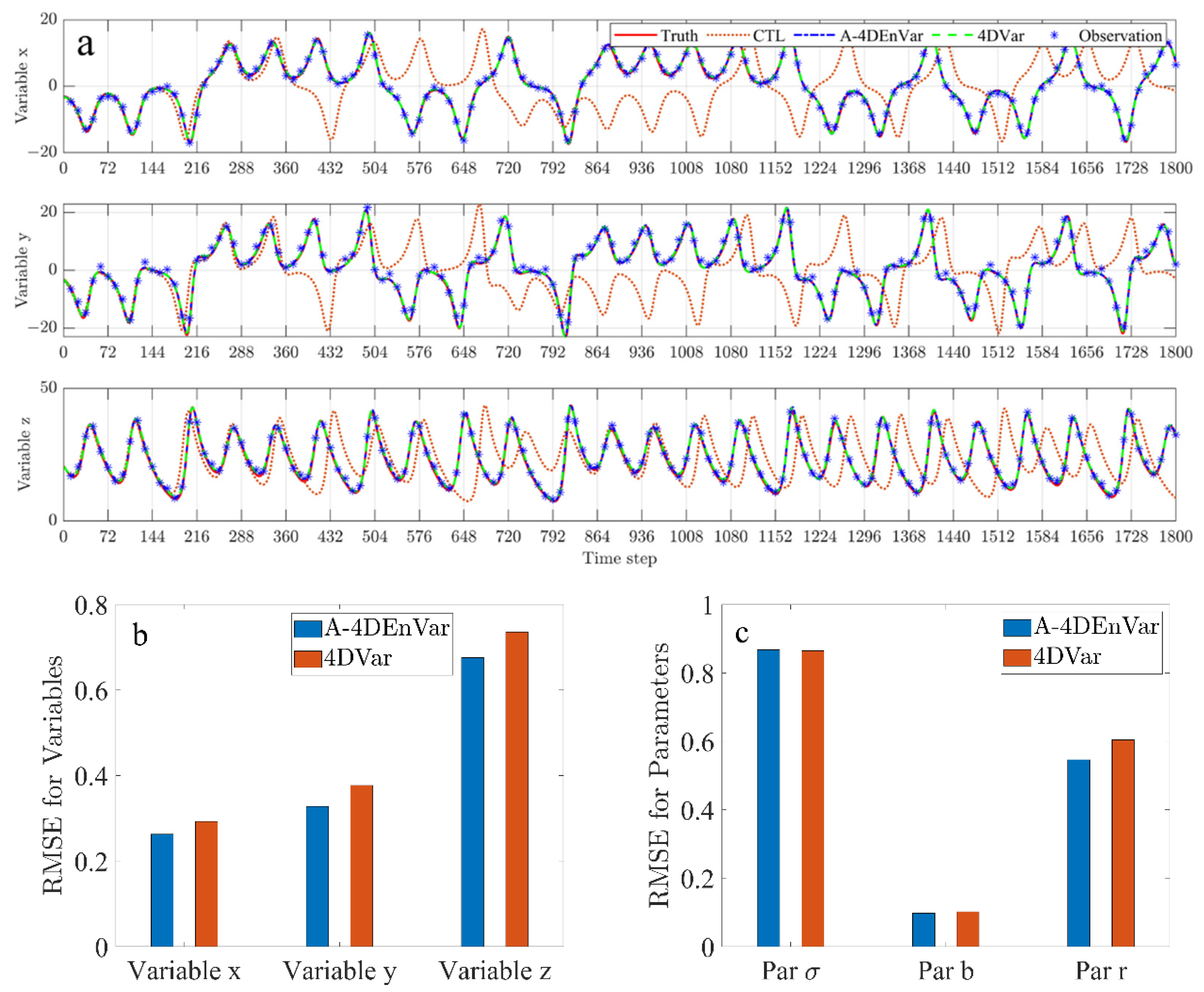
Here, the ensemble size is set to be 50 to validate the performance of A-4DEnVar in full rank. To test the performance of the algorithm, 100 experiments were produced using both A-4DEnVar and conventional 4DVar. In these experiments, the initial conditions for state variables, parameters, and observations are set to be the same for both A-4DEnVar and 4DVar (but they are different values in the 100 experiments). A model control run solution (labeled as CTL) without any data assimilation or correction is also presented.
The results (
Figure 2a shows the solutions only in the first 25 windows from one experiment) indicate the effectiveness of A-4DEnVar.
Figure 2b shows the mean RMSE of the conventional 4DVar algorithm and A-4DEnVar algorithm in all 100 experiments. Although the RMSE of A-4DEnVar is slightly less than that of 4DVar, both algorithms assimilate the information from observations so that the analysis RMSE for each variable is less than the standard deviations of observations, the unit of which is mentioned above. It is shown that both algorithms perform well under the experiment setting. In
Figure 2c, the RMSEs of parameters
and
from A-4DEnVar are less than that from 4DVar. However, 4DVar performs slightly better than A-4DEnVar on the parameter
.
Due to the complex manifold structure caused by the high nonlinear model, the global minimum of the cost function is difficult to achieve through gradient based optimal methods. The chaos of the Lorenz model makes the optimization even more difficult so that a small perturbation in the gradient would lead to another local minimum of the cost function. Considering that the motivation of A-4DEnVar is replacing the adjoint models with these estimated temporal cross error covariances, these estimations can be close enough to their true values but cannot be the same. The gradient directions calculated from adjoint models in 4DVar are slightly different from what was estimated in A-4DEnVar. Therefore, the RMSE obtained by the two data assimilation schemes might be slightly different from each other. In our conclusions, we do not emphasize whether the performance of 4DVar or that of A-4DEnVar is better, but only state that their performances are all acceptable and are equivalent to each other.
The computational cost also influences the usage of both methods. The computing burden for A-4DEnVar is mainly from integrating ensembles. For conventional 4DVar, the burden is mainly from the calculation of adjoint models. Empirically, running the adjoint model often costs about 6 to 10 times the computational resources of the forward dynamic model. Therefore, if every ensemble member is updated in each iteration, it would be cheaper to implement A-4DEnVar when the ensemble size is less than 10. However, it also should be noticed that regenerating or updating ensembles is only necessary if ensembles are not close to the background. For example, updating the ensembles after several iterations of increments is acceptable when the nonlinearity is limited. Therefore, it is possible for A-4DEnVar to further reduce its computing costs in practice. What also should be emphasized is that, to calculate the gradient, one has to store the value of state variables increments in every time step in 4DVar. In contrast to it, A-4DEnVar only stores the values of state variables where the observations are located. Considering the dimension of the state variables is often much larger than that of observations, A-4DEnVar saves most storage spaces. Besides, the proposed A-4DEnVar is an ensemble-based method, and it can be easily implemented in operational parallel systems to save time.
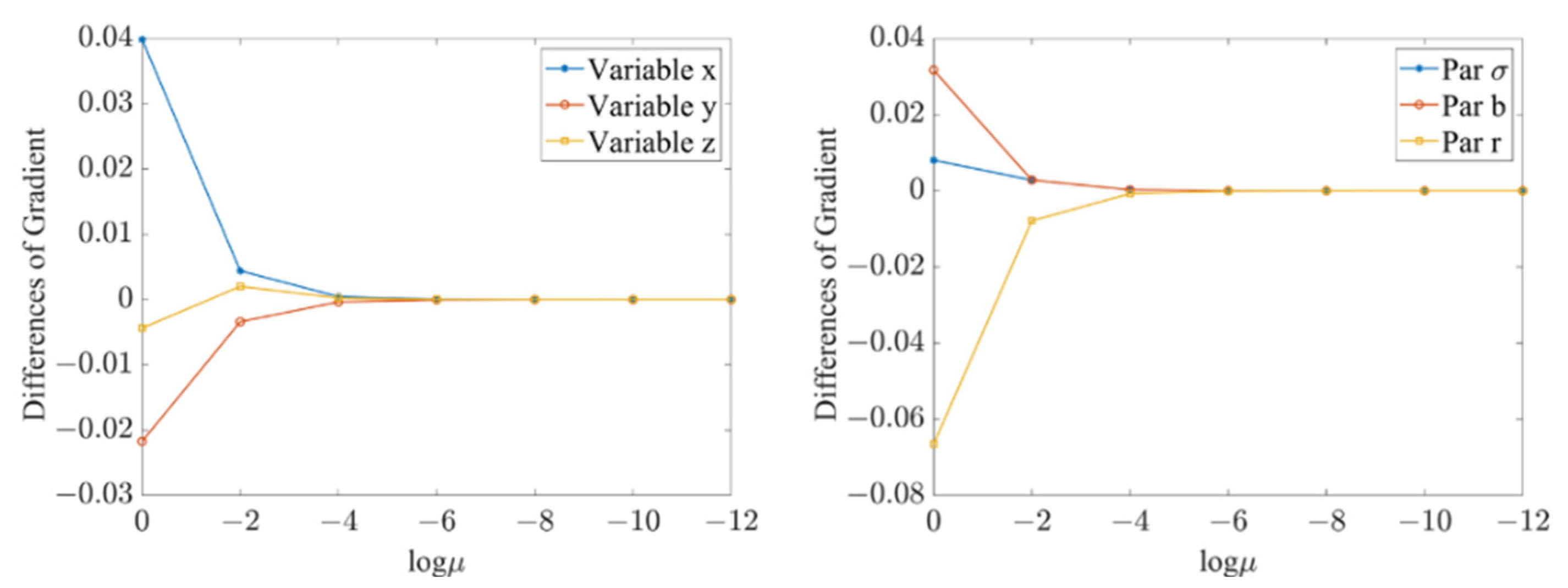
The usage of factor
to control the value of perturbations and generate ensemble members is an important difference between A-4DEnVar and 4DEnVar methods.
Figure 3 shows the difference between the gradients (in the first iteration step) calculated by A-4DEnVar and the traditional 4DVar method with the change of
. It is shown that, in Lorenz-63 model, only if the factor is less than
which is far less than the value of the background error covariance used in other 4DEnVar methods, the gradients (for both variables and parameters) obtained from A-4DEnVar are close enough to that from traditional 4DVar.
3.3. Model Sensitivities with Respect to Observation Period, the Length of Data Assimilation Windows and Ensemble Size
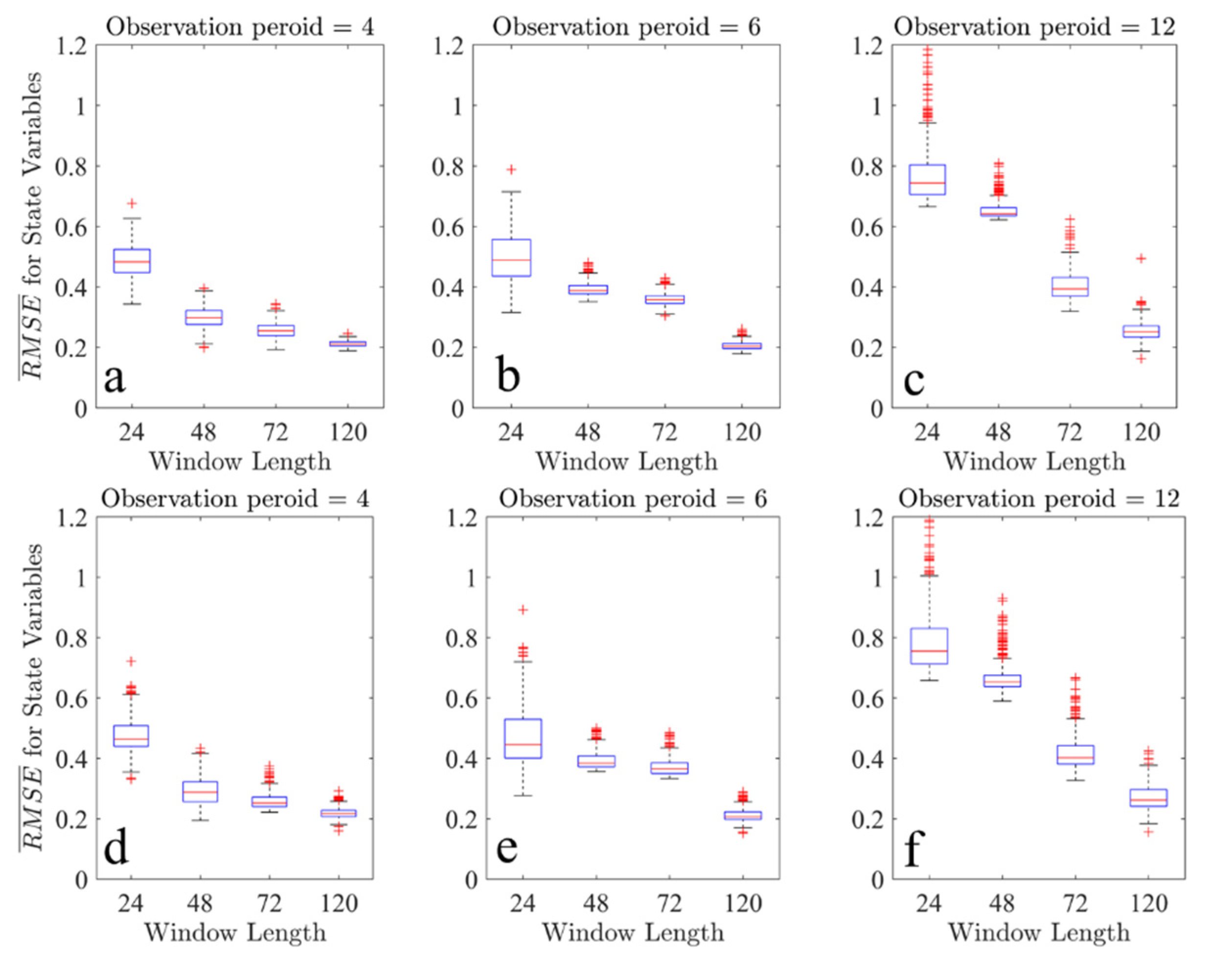
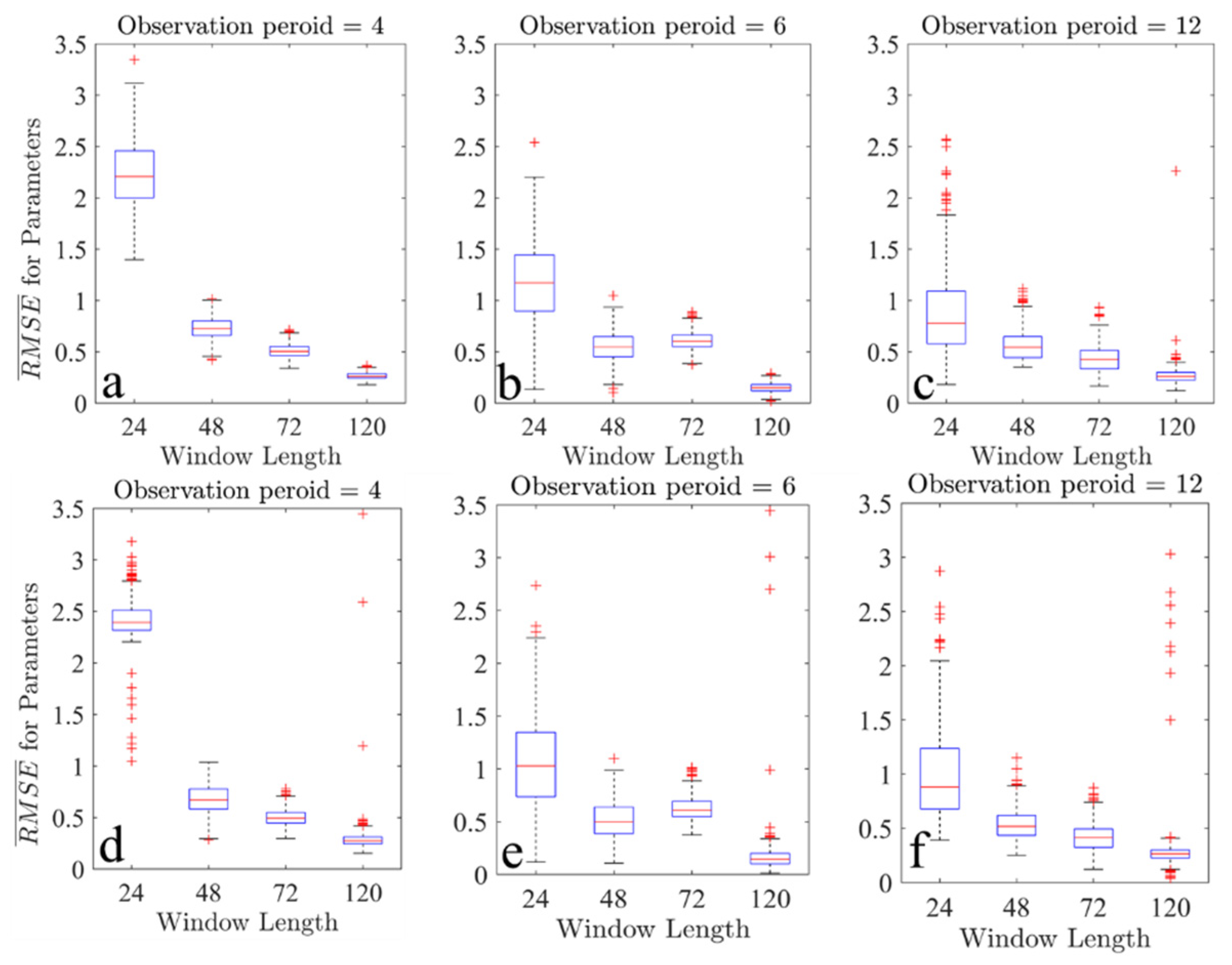
Since the nonlinearity of operational NWP systems increases with the length of the assimilation window, it is of great importance to point out the assimilation capability of A-4DEnVar with different window lengths and observation periods. In this set of experiments, the window of length 24, 48, 72, and 120 steps with observation periods 4, 6, and 12 steps are conducted. Each experiment is carried out 500 times to test the statistical performance and robustness. Again, the initial conditions for state variables, parameters, and observations are set to be the same for A-4DEnVar and 4DVar, but they are different values in these experiments.
The RMSEs of state variables as a function of window lengths and observation periods are presented by box plot in
Figure 4. On each box, the central mark indicates the median, and the bottom and top edges of the box indicate the 25th and 75th percentiles, respectively. The whiskers extend to the most extreme data points not considered outliers, and the outliers are plotted individually using the red cross-marker symbol. It can be seen that for experiment settings, most RMSEs of variable states are less than 1.0. The outliers are mainly because of the random choice of backgrounds, and the algorithms find a local minimum. For a fixed window length, the mean of assimilation RMSEs increases with the observational period. The best performance occurs when the window is about 120 time steps. If the window is too short, the lack of observational information also results in large RMSEs. When the assimilation window is 24 steps and the observation period is 24 steps (not shown here), the RMSE is greater than the standard deviation of the observational noise, which indicates the failure of data assimilation.
For parameters in
Figure 5, a shorter observational period does not achieve a smaller RMSE. In this case, we find that the minimum point of the cost function is different from the truth because of the interaction between state variables and parameters and the noises contained in observations. Since both A-4DEnVar and 4DVar converge to this point, parameters with high RMSEs are obtained. However, the trajectories are almost the same as the truth. Another suit of experiments (not shown here) which only optimize parameters with perfect initial conditions shows that the interactions can be alleviated but cannot be completely eliminated. Both in
Figure 4 and
Figure 5, the experiments carried out by 4DVar using the same settings also lead to similar results and demonstrate the equivalence of A-4DEnVar and 4DVar.
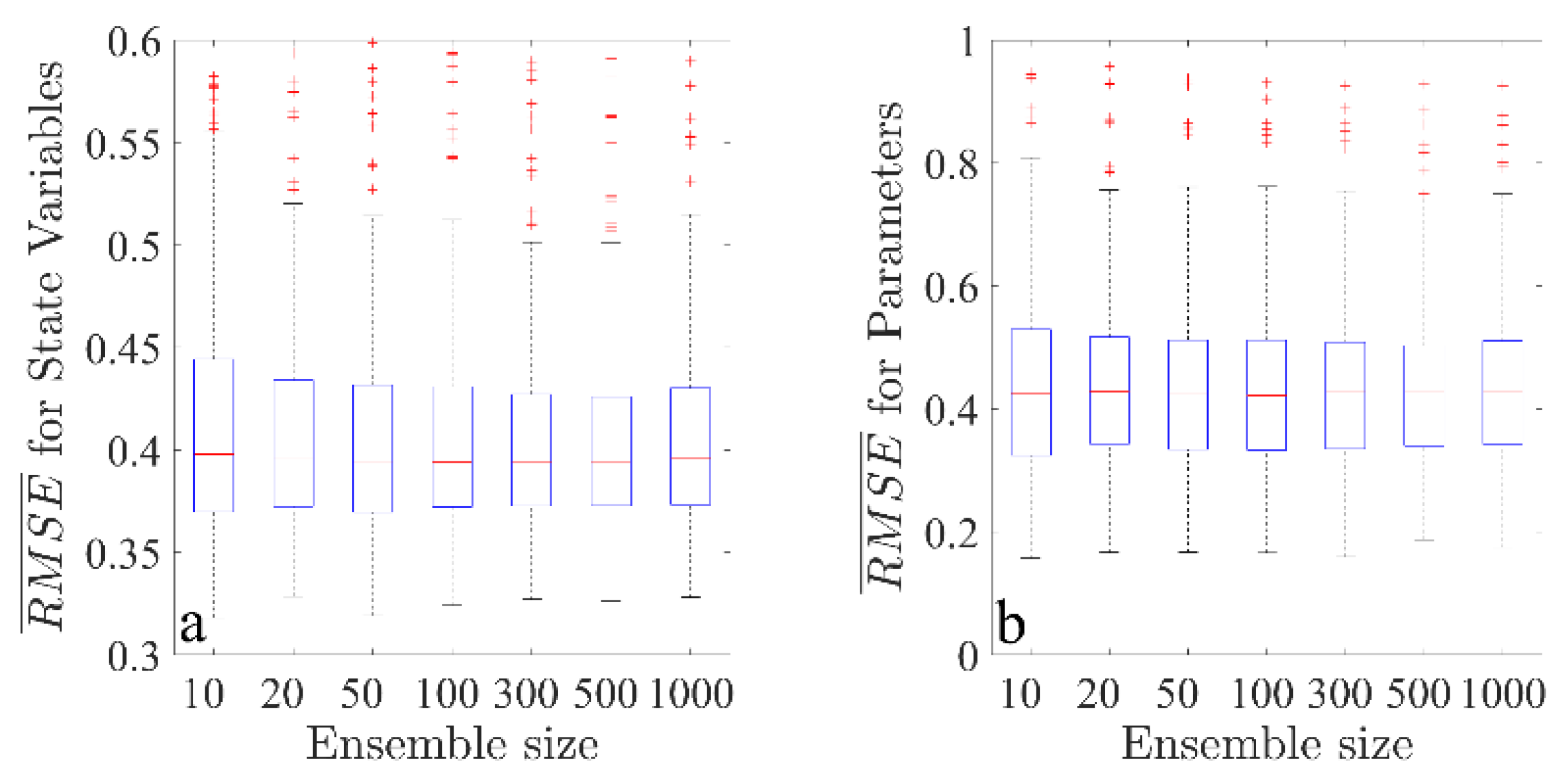
In the last set of experiments, we consider the impact of ensemble size on the performance of A-4DEnVar. Generally speaking, the dimensions of variable states in the operational NWP system are huge. It is necessary to evaluate the required ensemble size for data assimilation. However, we only consider a simple model with full rank ensembles here. Because the Lorenz-63 chaos system has six degrees of freedom, to implement data assimilation, the ensemble sizes are chosen as 10, 20, 50, 100, 300, 500, and 1000, while the window length and observational period are set to be 72 and 12 steps as in the preliminary experiment. Each experiment is also repeated 500 times to demonstrate the statistical performance of the A-4DEnVar under the same settings used above. The
results for variables and parameters are shown in
Figure 6.
Although the RMSEs for each variable change a little with different ensemble size, it is clear that all RMSEs are less than observation variance, which shows the effectiveness of the proposed algorithm. The A-4DEnVar is not sensitive to the ensemble sizes for the Lorenz model with full rank ensembles. In fact, the key to A-4DEnVar is estimating the adjoint models by ensemble perturbations. The performance of A-4DEnVar depends on the precision of these estimations. Theoretically, it is the magnitude of ensemble perturbations rather than the ensemble sizes influence the estimation of adjoint models. The experiment results shown in
Figure 6 also indicate that RMSE does not improve significantly with the increase of ensemble sizes. While the dimension of the NWP system is large, it is often impossible to generate enough ensemble members. Hence, the localization methods should be introduced to alleviate spurious correlations between state variables. However, we do not focus on the issue in this paper and our related studies are also on the way.


