Article

Tropopause Characteristics Based on Long-Term ARM Radiosonde Data: A Fine-Scale Comparison at the Extratropical SGP Site and Arctic NSA Site

by
Jinqiang Zhang
1,2,3
1
Key Laboratory of Middle Atmosphere and Global Environment Observation, Institute of Atmospheric Physics, Chinese Academy of Sciences, Beijing 100029, China
2
Collaborative Innovation Center on Forecast and Evaluation of Meteorological Disasters, Nanjing University of Information Science & Technology, Nanjing 210044, China
3
College of Earth and Planetary Sciences, University of Chinese Academy of Sciences, Beijing 100049, China
Atmosphere 2022, 13(6), 965; https://doi.org/10.3390/atmos13060965
Submission received: 19 May 2022 / Revised: 11 June 2022 / Accepted: 13 June 2022 / Published: 14 June 2022
(This article belongs to the Special Issue Feature Papers in Atmosphere Science)

Abstract

:
The variations in the characteristics of the tropopause are sensitive indicators for the climate system and climate change. By using Atmospheric Radiation Measurement (ARM) radiosonde data that were recorded at the extratropical Southern Great Plains (SGP) and Arctic North Slope of Alaska (NSA) sites over an 18-year period (January 2003 to December 2020), this study performs a fine-scale comparison of the climatological tropopause features between these two sites that are characterized by different climates. The static stability increases rapidly above the tropopause at both sites, indicating the widespread existence of a tropopause inversion layer. The structures of both the tropopause inversion layer and the stability transition layer are more obvious at NSA than at SGP, and the seasonal variation trends of the tropopause inversion layer and stability transition layer are distinctly different between the two sites. A fitting method was used to derive the fitted tropopause height and tropopause sharpness (λ). Although this fitting method may determine a secondary tropopause rather than the primary tropopause when multiple tropopause heights are identified on one radiosonde profile, the fitted tropopause heights generally agree well with the observed tropopause heights. Broad tropopause sharpness values (λ > 2 km) occur more frequently at SGP than at NSA, resulting in a greater average tropopause sharpness at SGP (1.0 km) than at NSA (0.6 km). Significant positive trends are exhibited by the tropopause heights over the two sites, with rates of increase of 23.7 ± 6.5 m yr−1 at SGP and 28.0 ± 4.0 m yr−1 at NSA during the study period.

1. Introduction

The tropopause, which marks the top of the troposphere and separates it from the overlying stratosphere, is distinct from either of these layers in regard to both its radiative properties and dynamics and its chemical transport characteristics [1,2]. Detailed investigations of the tropopause features are important for understanding the global climate system and climate change [3,4,5]. The tropopause is thermally defined based on the variation in the vertical temperature lapse rate [6]. Nevertheless, for specific research purposes, several other dynamic and chemical definitions of the tropopause have been proposed by using potential vorticity thresholds [7,8] and the concentrations of trace gases such as ozone and water vapor [9,10].
Based on high-resolution radiosonde measurements, a tropopause inversion layer (TIL) that is characterized by a strong temperature increase above the tropopause was found at two midlatitude sites in southern Germany [11]. Subsequently, the TIL was also identified by radiosonde measurements at other sounding stations [12,13], by reanalysis data and model simulations [14,15], and by satellite retrievals [5,16]. Although previous studies have documented some of the characteristics of the TIL, the physical mechanism that is responsible for its existence is still subject to debate and has yet to be clarified. To date, two main mechanisms have been proposed to explain the development and maintenance of the TIL, i.e., dynamic processes [12,17,18,19] and radiative effects that are associated with water vapor and ozone near the tropopause [5,20,21]. Researchers have also suggested that the TIL originates from a synergetic effect of radiative and dynamic processes occurring at both stratospheric and tropospheric levels [16,22].
Although there has been increased interest in the global tropopause in recent years, resulting in a few of the studies that are mentioned above, observations of the fine-scale tropopause characteristics are still needed to better understand the dynamic and chemical transitions between the troposphere and stratosphere, especially given that the formation mechanism of the TIL remains unclear and that different processes may be important in different regions [23]. Based on the consideration, this paper employs long-term radiosonde data at two sounding sites in the midlatitudes and Arctic with the main goal being to quantify and compare the detailed features of the tropopause, including the climatology of the tropopause on various temporal scales, the stability transition layer around the tropopause, and the sharpness of the tropopause in the two different climatic zones. Moreover, the variation trend of the tropopause height is discussed given that the variability in the tropopause height is suggested to be a sensitive indicator of anthropogenic climate change [4]. The remainder of this paper is organized as follows. Section 2 describes the data and methods that were used in this study. The tropopause characteristics at two different climatic sites are quantified and compared in Section 3. Then, the main conclusions are summarized in Section 4.

2. Sites, Data and Methods
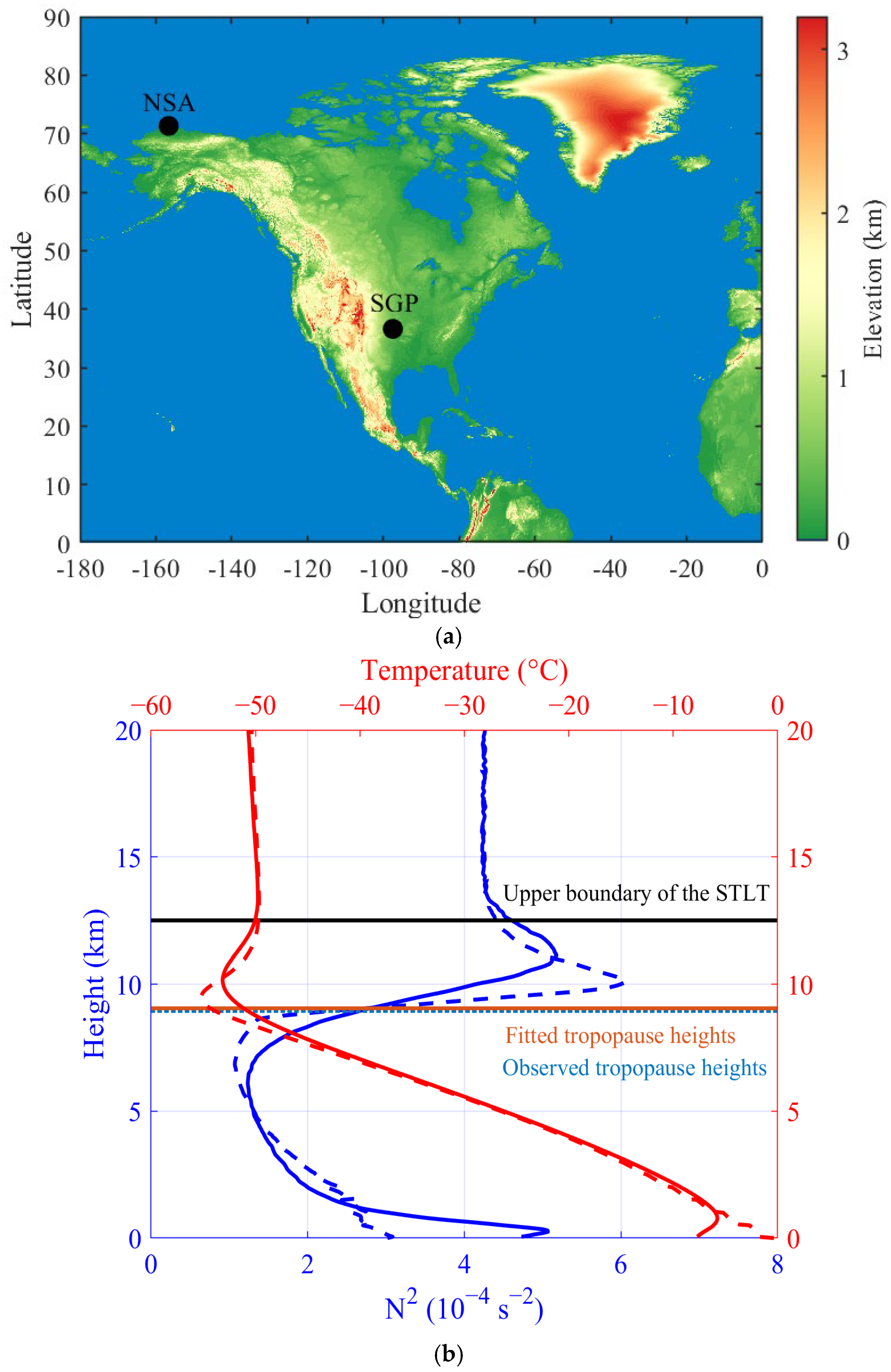
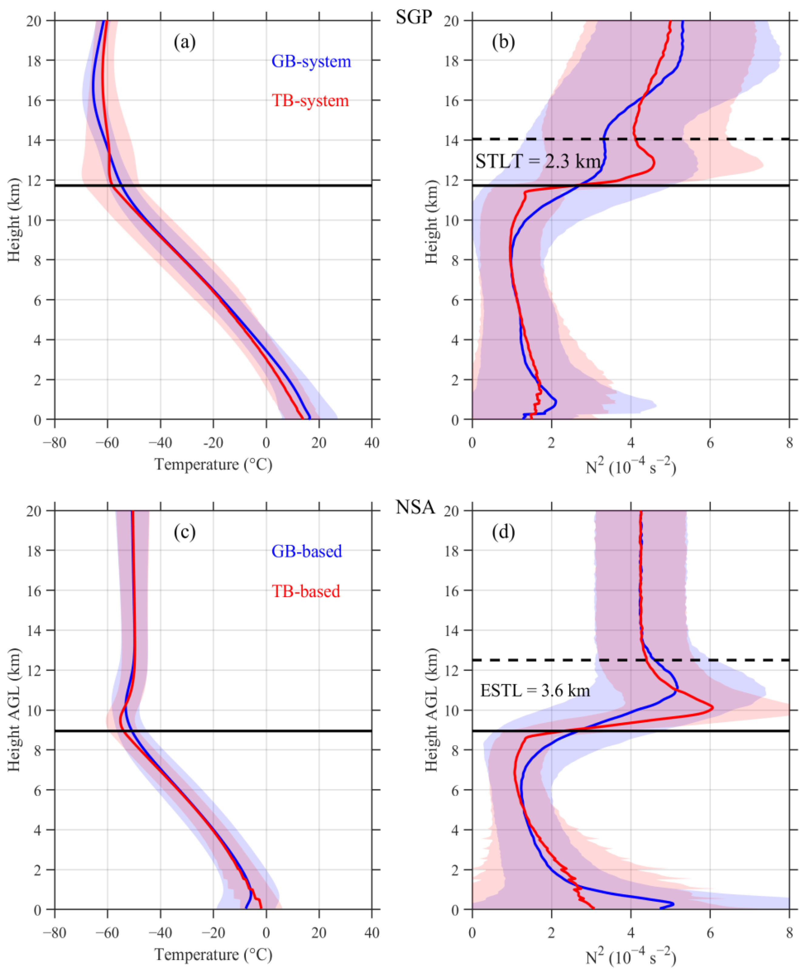
2.1. Sites and Data

In this study, radiosonde data that were recorded over an 18-year period (January 2003 to December 2020) at the Atmospheric Radiation Measurement (ARM) Southern Great Plains (SGP) Central Facility site in north-central Oklahoma (36.6° N, 97.5° W, 315 m above sea level) and the North Slope of Alaska (NSA) site near Barrow (71.3° N, 156.6° W, 8 m above sea level) (Figure 1) were used to derive the climatological features of the tropopause. As the first ARM field measurement site, SGP is the world’s largest and most extensive climate research facility and is perfect for investigating the atmospheric processes in the midlatitudes, whereas NSA is an ideal high-latitude site for examining the rapidly changing atmosphere and climate in the Arctic.
Routine radiosonde launches were chiefly performed four times a day at 0530, 1130, 1730, and 2330 UTC at SGP and primarily performed at least twice per day at 0530 and 1730 UTC at NSA. A radiosonde measures the pressure, temperature, humidity, wind speed, and wind direction at a high vertical resolution of ~10 m. Only radiosonde profiles with maximum altitudes reaching above 20 km were selected in this study to ensure that the measurements exceed the primary tropopause.

2.2. Methods

According to the algorithm in WMO [6], the thermal tropopause that was used in this study is defined as the lowest level where the temperature lapse rate falls below 2 K km−1 and where the average temperature lapse rate between this level and all the higher levels within 2 km remains below this value. The thermal tropopause is directly related to the enhanced static stability [5,16,20,22] that is usually represented by the Brunt-Väisälä frequency N or its square as follows in Equation (1):
N 2 = g θ θ z = g T T z + Γ d
where g is the constant acceleration due to gravity, θ is the potential temperature, T is the temperature, z is the altitude, and Γ d = 9.8 °C km−1 is the dry adiabatic lapse rate.
Birner et al. [11] and Birner [12] showed that, due to the substantial seasonal variability of the tropopause height at a given site, averaging the TIL in a ground-based vertical coordinate system (GB-system) smears it out, making the TIL difficult to identify, whereas the TIL is a ubiquitous and clear feature in a tropopause-based vertical coordinate system (TB-system). In the TB-system, each radiosonde profile is calculated with respect to the time-dependent tropopause height by Equation (2):
z ˜ = z z TP + z TP ¯
where z ˜ is fixed in time with respect to the tropopause for each radiosonde profile, z is fixed in time with respect to the ground level for each radiosonde profile, z TP is the tropopause height with respect to the ground level determined by each radiosonde profile, and z TP ¯ denotes the time-averaged height of the tropopause with respect to the ground level from all the radiosonde profiles on various temporal scales (such as month, season, and year) in question.
The atmospheric stability transitions from weak in the troposphere to strong in the stratosphere [24,25]. Based on this phenomenon, Bell and Geller [13] defined a stability transition layer around the tropopause (STLT), i.e., the region over which the static stability relaxes from its overshoot value at the tropopause to its local minimum in the stratosphere (where dN 2 dz = 0 ). The depth of the stability transition layer that was adopted from Bell and Geller [13] is calculated in this study. Moreover, to identify the tropopause sharpness (λ), which reflects the thickness of the transition layer from the troposphere to the stratosphere, this paper applies an idealized smooth step-like function to the observed profiles of the static stability N using a nonlinear curve fitting method [26], as defined below in Equation (3):
N z = N trop + N strat N trop 2 [ 1 + tanh ( 2 ( z z 0 ) λ ) ]
where N trop and   N strat are the typical values of N in the troposphere and stratosphere, respectively; tan h represents the hyperbolic tangent function; the tropopause height is taken to be the transition midpoint at z 0 ; and the tropopause sharpness is denoted λ . The above four parameters are calculated for each static stability profile by using a least-squares fitting method. To reduce a substantial amount of discretization-induced noise and preserve most of the detailed structure, the static stability profiles that were calculated from the radiosonde data are subsampled from a high vertical resolution of ~10 m to a lower vertical resolution by interpolating at an interval of 50 m [27,28]. The best initial estimates for the above parameters, i.e.,   N trop = 0.0 s−1,   N strat = 25.0 × 10⁻³ s−1, and λ = 1 km, are adopted from Homeyer et al. [26]. The initial estimate for the tropopause height z 0 is taken as the value that is calculated from each radiosonde profile using the algorithm in WMO [6]. The tropopause sharpness and stability transition layer that are used in this study can express the transition between the troposphere and stratosphere from different perspectives as follows. The tropopause sharpness should characterize primarily areas with dramatic changes in stability around the tropopause, whereas the stability transition layer may additionally include a wider area with a slowly decreasing stability until a local minimum is reached in the stratosphere. In this regard, the tropopause sharpness may be recognized as part of the stability transition layer. A schematic of the tropopause profiles that were derived from the NSA site is shown in Figure 1 which marks the relevant heights and systems that were used in the study, including the temperature and stability profiles in the GB-system and TB-system, the observed tropopause height (recognized as the bottom boundary of the STLT), the upper boundary of the STLT, and the fitted tropopause height.

3. Results

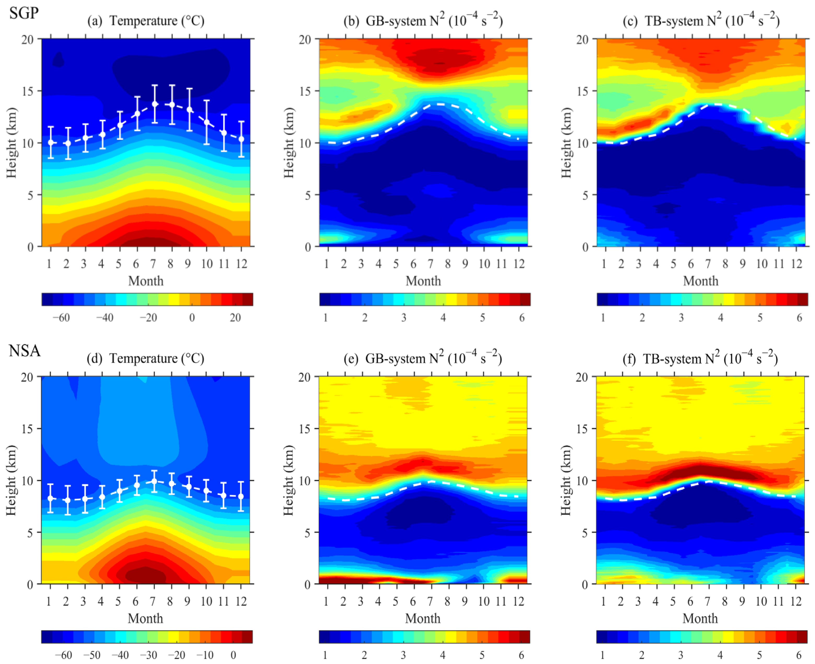
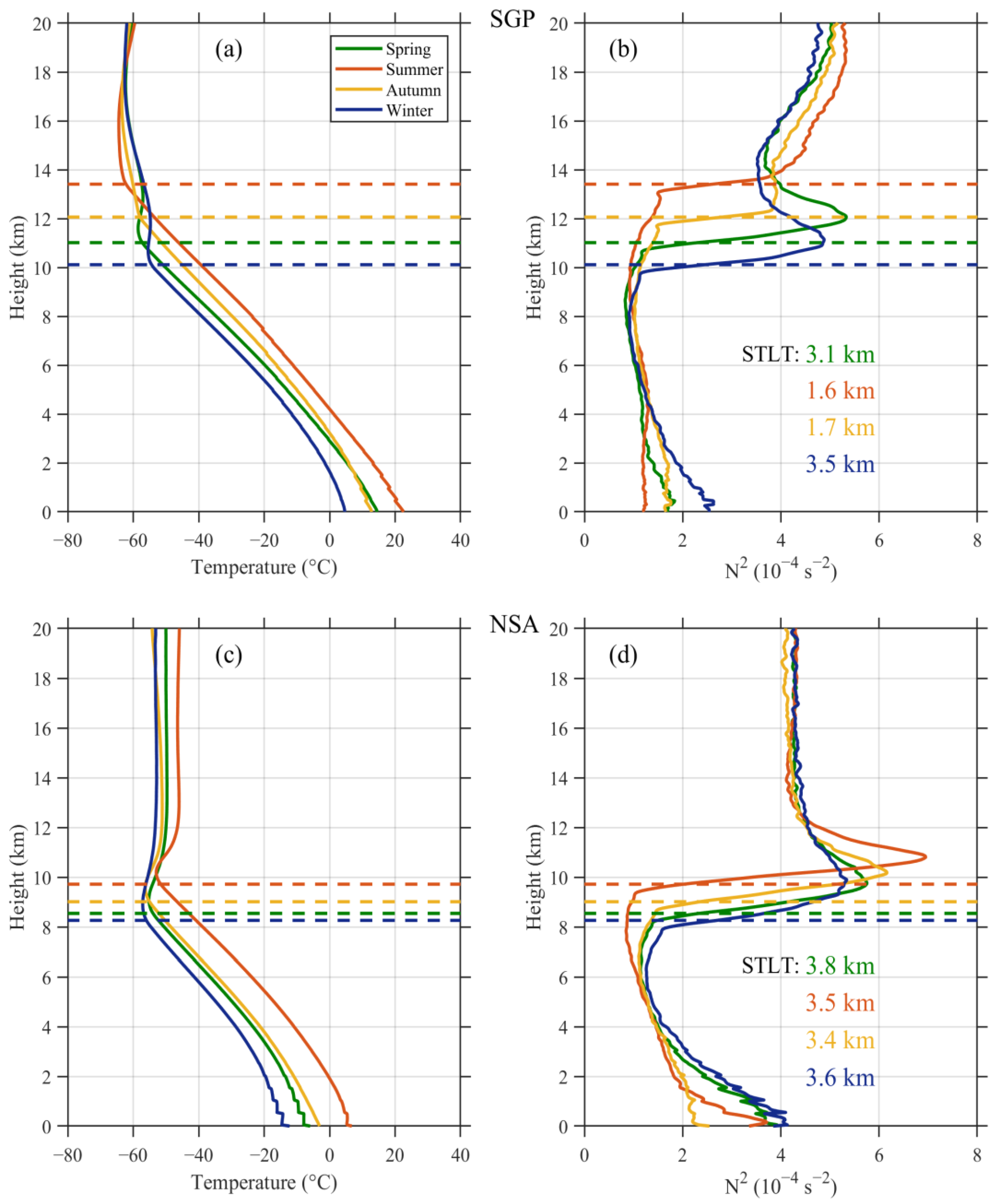
3.1. Climatology of the Tropopause Structure on Various Temporal Scales

Figure 2 shows the annually averaged climatologies of the TB-system temperature and stability during 2003–2020 at the SGP and NSA sites, and the GB-system profiles are presented for a comparison. The average tropopause is higher at SGP (11.7 km) than at NSA (8.9 km) due to the different atmospheric conditions between the two sites [29]. Consistent with the findings of Birner et al. [11] and Birner [12], the variation trends of both the temperature and the stability above the tropopause are larger in the TB-system than in the GB-system at both sites. A closer look at the TB-system reveals that the obvious temperature increase above the tropopause corresponds to a growth spurt in the vertical stability profiles until a maximum is reached, which indicates the existence of a strong TIL. The depths of the stability transition layer are also noted in Figure 2, which are 2.3 km at SGP and 3.6 km at NSA. The variation trends of the stability above the tropopause are clearer at NSA than at SGP, resulting in a visually distinct upper boundary of the STLT at NSA, although the identifying method is valid at both sites. Bell and Geller [13] showed that the stability transition layer increased monotonically in depth from ~1 km at low latitudes to ~4 to 5 km at high latitudes. Similar to their results, the stability transition layer is thinner by 1.3 km at SGP in the midlatitudes than at NSA in the Arctic. Furthermore, in addition to the TIL, an evident temperature inversion layer is also observed near the ground at the NSA site [29]; however, an examination of this layer, which is induced by ubiquitous surface radiative cooling, is beyond the scope of the current study.
The monthly averaged climatologies of the temperature and stability at SGP and NSA are visualized in Figure 3. The SGP site exhibits evident monthly changes in both temperature and stability, resulting in clear variations in the tropopause height and TIL structure. The tropopause is uplifted from January (10.0 km) to its maximum altitude in July (13.7 km) at SGP, and a local stability maximum generally occurs within 2 km above the tropopause. The TIL is distinctly stronger in cold months than in warm months, as the TIL is much weaker and thinner in the latter. At NSA, the tropopause height is fairly constant throughout the year, although it is slightly higher in warm months, when more radiation energy is generated during the polar days, than in cold months with the onset of polar nights [30,31]. In sharp contrast to that at SGP, the TIL at NSA is stronger in warm months than in cold months. Again, the TIL is much clearer in the TB-system than in the GB-system at both sites. The seasonal variation in the tropopause height is stronger at SGP than at NSA, which results in less agreement on the stability structure between the TB-system and GB-system above 15 km at SGP than at NSA. In addition, a comparison between the two sites reveals that the TIL structure seems to be more obvious at NSA than at SGP, as indicated by a strong jump in the stability at NSA. Figure 4 further shows the seasonal variations (spring: March-May; summer: June–August; autumn: September-November; winter: December–February) in the TB-system at SGP and NSA. At both sites, the tropopause is highest in the summer, followed by (in decreasing order) that in autumn, spring, and winter. The seasonal variation in the tropopause height is weaker at NSA than at SGP. Although the TIL structure is visible in all four seasons, fine-scale discrepancies arise in various seasons and between the two sites, as shown by the variabilities in the temperature and stability profiles above the tropopause. In particular, the depth of the stability transition layer presents a significant seasonal fluctuation at SGP, with a maximum of 3.5 km in winter and a minimum of 1.6 km in summer, whereas that of the stability transition layer is rather constant at NSA (approximately 3.5 km) throughout the year.

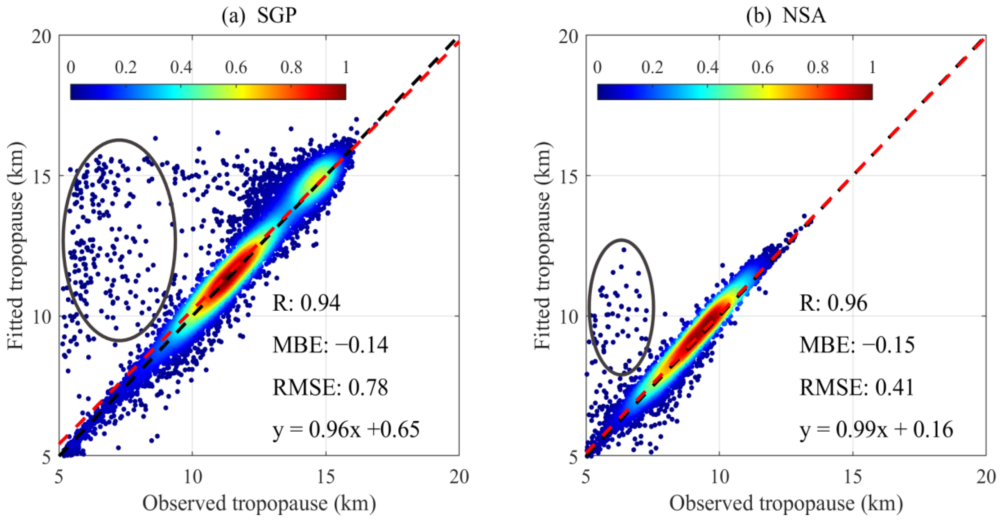
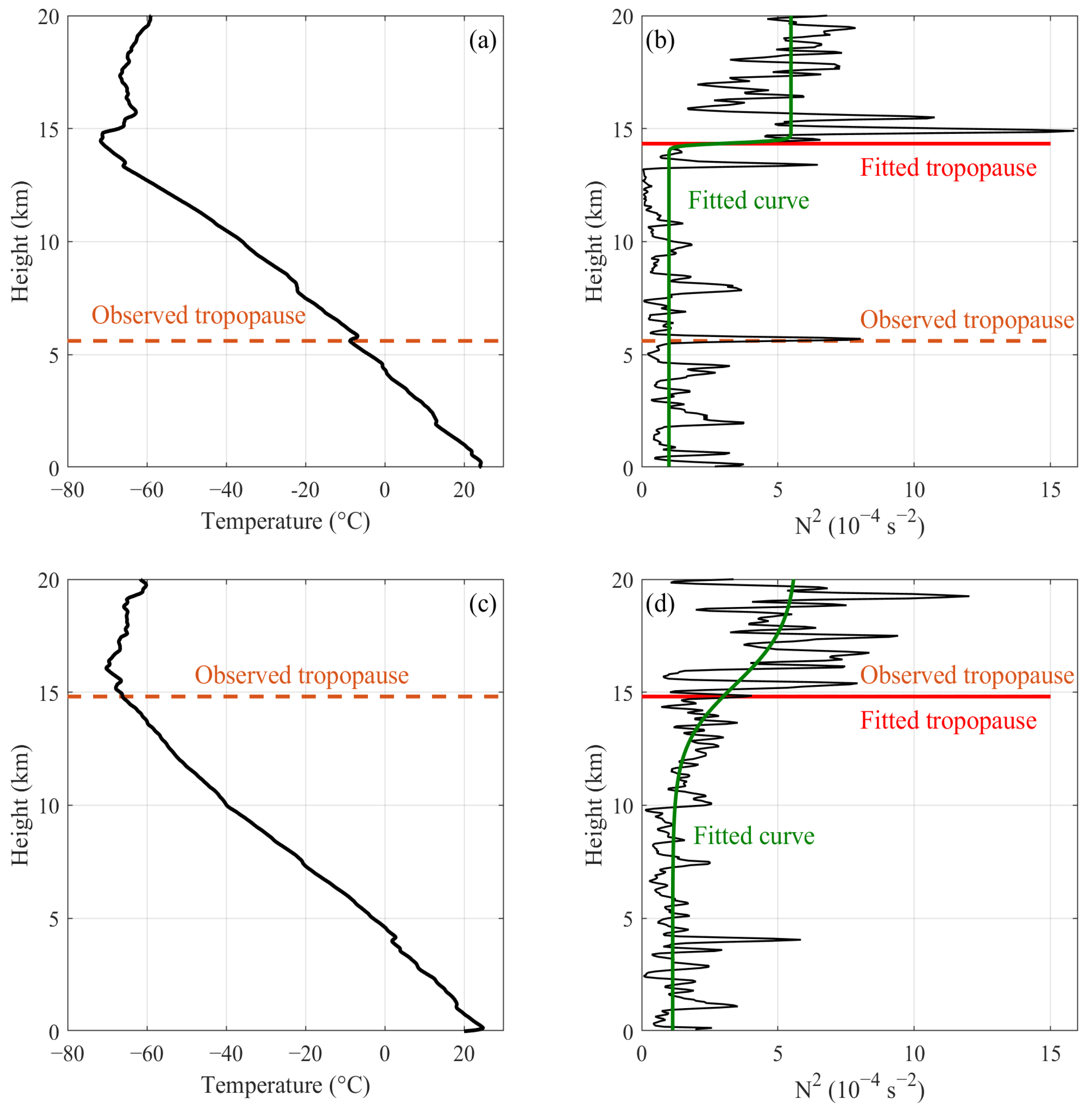
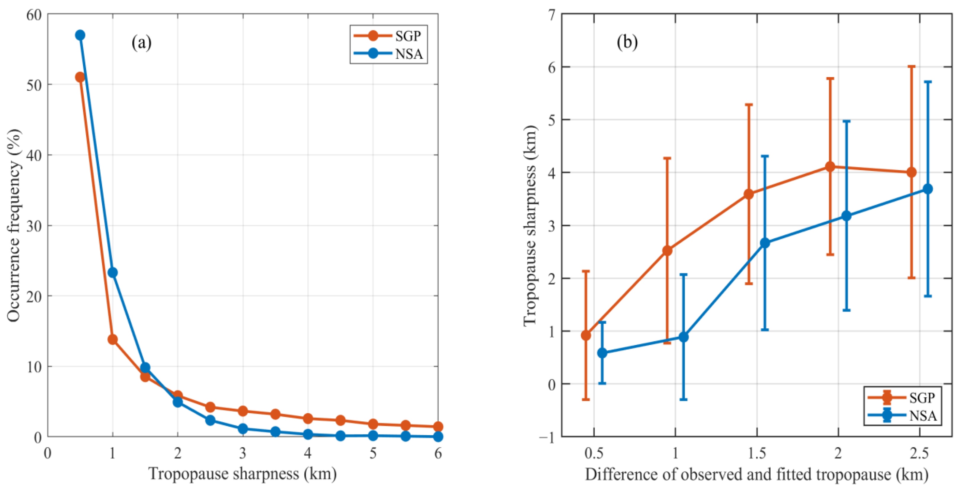
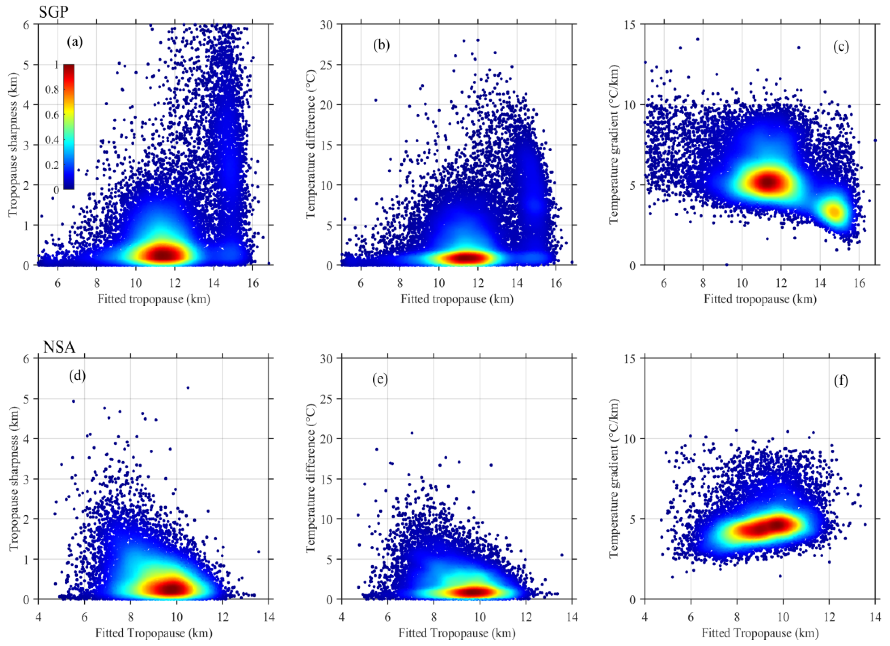
3.2. Fitting-Derived Tropopause Features

The fitting method adopted from Homeyer et al. [26], which applies an idealized smooth step-like function to the observed profiles of the static stability using a nonlinear curve fitting method, is used to derive the tropopause height and tropopause sharpness in this section. Figure 5 shows a comparison between the observed tropopause heights that were obtained by the method of WMO [6] and the tropopause heights that were derived from the fitting method at SGP and NSA. Overall, the tropopause heights that were derived from these two methods agree well, as indicated by the majority of data points falling along the 1:1 line. The percentages are 86.9% at SGP and 91.4% at NSA, respectively, for the data points with the absolute difference <0.5 km between the observed and fitted tropopause heights. Furthermore, the correlation coefficient (R), mean bias error (MBE; observed-fitted), and root mean square error (RMSE) between the two tropopause retrievals are 0.94, −0.14 km, and 0.78 km at SGP, respectively, and 0.96, −0.15 km, and 0.41 km at NSA. However, as delineated within the ellipses in Figure 5, a few outliers were detected above the 1:1 line. Further investigation revealed that these points with large differences between the two tropopause retrievals are due to a mismatch in the tropopause height resulting from multiple detected tropopause heights on one radiosonde profile, as explained by the case study that is presented in Figure 6. In this case, the radiosonde detects a strong temperature inversion at approximately 6 km, which is likely caused by a tropopause fold that is associated with a deep stratospheric intrusion [26,32]. The first tropopause height was determined to be 5.6 km by the WMO method. However, the fitting method identified a second tropopause at 14.3 km. The double tropopause that was calculated by the WMO criterion is most frequent in the middle latitude region, such as SGP station in this study. The first tropopause is generally formed by the dynamical factors in the middle latitude region. Similar cases for multiple detected tropopause heights (as shown in Figure 6) are less frequent at NSA than at SGP, resulting in better agreement between the observed and fitted tropopause heights at NSA than at SGP (as shown in Figure 5). The outliers that were induced by such tropopause mismatches were excluded from the following analysis. At a more detailed level at SGP, a relatively dense area occurs at about 14 km where the fitted method looks systematically overestimated, which may be associated with an increased tropopause transition layer that is related to weak variation in the static stability around the tropopause region for these cases. Apart from the above outliers, most of the data points are normal cases that are characterized by close observed and fitted tropopause, as shown by a case study in Figure 6 with observed and fitted tropopause almost overlapped at ~15 km.
Figure 7a shows the occurrence frequencies of the tropopause sharpness that was derived from the fitted method at both sites. Most values of the tropopause sharpness are less than 0.5 km, accounting for 51.0% and 57.0% at SGP and NSA, respectively, beyond which (tropopause sharpness >0.5 km) the occurrence frequency declines gradually. Homeyer et al. [26] divided the tropopause sharpness (λ) into two categories, i.e., narrow (λ ≤ 2 km) and broad (λ > 2 km), on the basis of the results from the continental United States for several months in 2008. The percentage of broad tropopause sharpness values at SGP in this study is 20.8%, which is relatively close to the magnitude (19.5%) in Homeyer et al. [26] at similar latitudes (35–40° N). Moreover, although their study areas uncovered the Arctic, Homeyer et al. [26] reported a decreasing frequency of broad tropopause sharpness values with increasing latitude. This latitude variation trend is affirmed by the results of this study, as shown by the broad tropopause sharpness occurring more frequently at the extratropical SGP (20.8%) than at the Arctic NSA (5.0%). Previous studies have suggested that frequently occurring broad tropopause sharpness in low latitudes may be associated with the dynamic and radiative characteristics of the tropical upper troposphere [33], while a broad tropopause sharpness might primarily exist in the midlatitudes within lower-stratospheric cyclonic flows [9,17]. The relationship between the tropopause sharpness and the absolute difference of the observed and fitted tropopause is presented in Figure 7b, revealing a clear variation trend at both sites in which the tropopause sharpness increases with an increasing absolute difference. The rapid variation in the static stability around the tropopause will generate narrow tropopause sharpness, and for these cases the fitted tropopause are generally consistent with the observed tropopause.
To investigate how the tropopause features vary with the tropopause height, density plots of the tropopause sharpness, temperature difference, and temperature gradient across the tropopause sharpness as a function of the fitted tropopause height are shown in Figure 8, in which the outlier points that were identified in Figure 5 are removed. The fitted tropopause is used in Figure 8 given that the tropopause sharpness, temperature difference, and temperature gradient are derived based on the fitted tropopause method. The temperature difference is defined as the difference between the temperature at the tropopause sharpness top (the altitude located a distance of λ above the fitted tropopause height) and the temperature at the tropopause sharpness base (the fitted tropopause height), whereas the temperature gradient is defined as the temperature difference divided by the tropopause sharpness. At SGP, the tropopause sharpness values are concentrated in areas where λ < 1 km near a tropopause height of ~11 km. Additionally, as shown by the vertical cluster of data that are distributed at tropopause heights of 14–16 km, a few data points exhibit relatively broad tropopause sharpness which should be associated with complicated dynamic processes and radiative effects around the tropopause in summer. Overall, the variation trend of the temperature difference with the tropopause height is generally similar to that of the tropopause sharpness. In contrast, the temperature gradient, which is predominantly distributed at tropopause heights of ~11 km and ~15 km, demonstrates a declining variation trend with increasing tropopause height. At NSA, the tropopause sharpness and temperature difference, which are concentrated at a tropopause height of ~10 km, also present similar variation trends with the tropopause height. The temperature gradient is widely concentrated between tropopause heights of 8 and 10 km and presents a smoothly increasing trend with an increase in the tropopause height. Overall, obviously different distributions are observed at NSA and SGP for one specific parameter as a function of the tropopause height, namely, the tropopause sharpness, the temperature difference, and temperature gradient. The average tropopause sharpness, temperature difference, and temperature gradient among all the data in Figure 8 are 1.0 km, 3.9 °C, and 5.2 °C km−1 at SGP, respectively, and 0.6 km, 2.5 °C, and 4.8 °C km−1 at NSA. The data averaged in each 1 km increment of the tropopause height are further compared in Figure 9. At SGP, both the tropopause sharpness and the temperature difference increase as the tropopause height increases, which results in a smoothly decreasing temperature gradient. On the contrary, the average variation in each parameter with the tropopause height at NSA is different from or even opposite that at SGP, i.e., decreasing tropopause sharpness and temperature difference but increasing temperature gradient with increasing tropopause height at NSA.

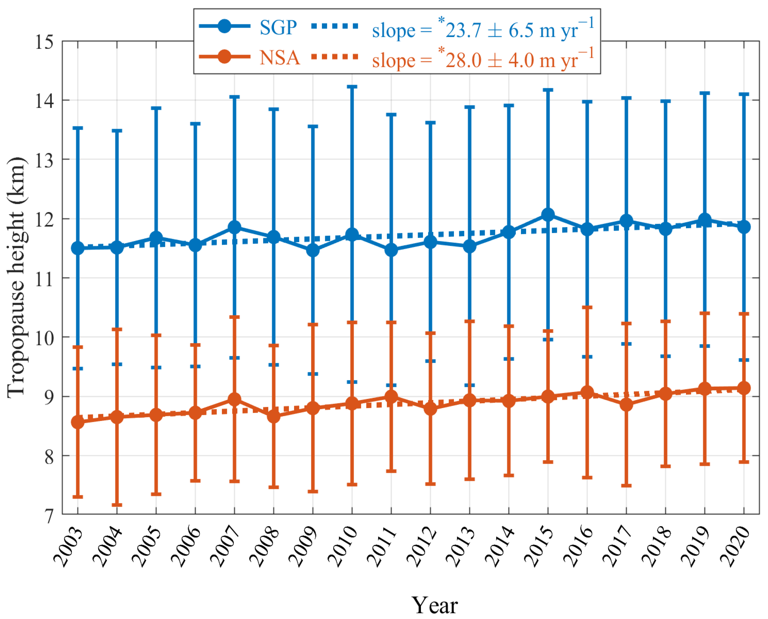
3.3. Variation Trend of the Tropopause Height

The long-term radiosonde measurements at the two sites allow the interannual variation trend of the observed tropopause height to be investigated, as shown in Figure 10. The annual variation in the tropopause height presents a significant positive trend during 2003–2020, with magnitudes of 23.7 ± 6.5 m yr−1 and 28.0 ± 4.0 m yr−1 at SGP and NSA, respectively. Although there is an overall increasing trend for tropopause height at SGP, it is less linear than the trend at NSA, as indicated by a larger standard deviation change at SGP across the study period. Seidel and Randel [2] indicated that the tropopause height trends over 1980–2004 were increasing at almost all of the radiosonde stations that they analyzed, yielding an estimated global trend of 6.4 ± 2.1 m yr−1. Therefore, the rates of increase at the two sites that were investigated in this study are approximately quadruple the global average magnitude that was reported in Seidel and Randel [2], although the research periods between this study and theirs are inconsistent. It has been suggested that changes in the tropopause height may be a sensitive indicator of anthropogenic climate change [4,34,35] and that the changes are accompanied by stratospheric cooling and tropospheric warming [2,4]. Owing to the unique feedbacks in the climate system, the phenomenon that is known as Arctic amplification has occurred throughout this region because the warming over this area is occurring two to three times faster than the global rate [36]. Continuous warming has led to a steady decline in Arctic sea ice cover over time [37]; therefore, it is reasonable to expect a positive feedback to Arctic warming, thereby accelerating its warming rate [38]. Our study preliminarily demonstrates that the rate of increase in the tropopause height has occurred faster at NSA than at SGP over almost the past two decades. Accordingly, further study is required to investigate whether this rate difference is associated with accelerated warming in the Arctic.

4. Conclusions

Precise knowledge of the fine-scale structure of the tropopause is important for thoroughly understanding stratosphere-troposphere exchanges and climate variability. By using long-term radiosonde data at the ARM extratropical SGP site and the Arctic NSA site, this study quantifies and compares the tropopause features in detail, including the tropopause structure, the stability transition layer, the sharpness of the tropopause, and the variation trend of the tropopause height, over these two sites that are situated within different climate zones. The main findings are summarized as follows.
The average tropopause is higher at SGP (11.7 km) than at NSA (8.9 km) due to the different atmospheric conditions at the two sites. The TIL is widespread over both sites but exhibits different temporal variation trends. The structure of the TIL is distinctly stronger in cold months than in warm months at SGP, whereas the reverse, i.e., where the TIL is much stronger in warm months than in cold months, holds true at NSA. The average stability transition layer is thinner at SGP (2.3 km) in the midlatitudes than at NSA (3.6 km) in the Arctic. In addition, the depth of the stability transition layer presents a significant seasonal fluctuation at SGP, in contrast to the relatively constant depth at NSA throughout the year. Compared to that at SGP, the agreement between the observed and fitted tropopause heights is better at NSA due to the lower occurrence frequency of tropopause mismatches at the latter site. Moreover, a broad tropopause sharpness occurs more frequently at SGP (20.8%) than at NSA (5.0%), resulting in a greater average tropopause sharpness at SGP (1.0 km) than at NSA (0.6 km). The tropopause height presents a significant positive trend at both sites during the 18-year study period, with rates of increase of 23.7 ± 6.5 m yr−1 and 28.0 ± 4.0 m yr−1 at SGP and NSA, respectively. Nevertheless, further research is needed to investigate whether the faster rate of increase in the tropopause height at the NSA site is associated with accelerated warming in the Arctic.
This study focuses on quantifying and comparing some fine-scale tropopause characteristics at two radiosonde sites that are characterized by different climates. The findings are expected to be valuable for understanding the transition features between the troposphere and stratosphere in the midlatitudes and Arctic. The physical mechanism that is responsible for the tropopause, for instance, the formation of the TIL, is still subject to debate and requires further investigation. However, the physical mechanism of the tropopause is too complicated to be acknowledged based only on the radiosonde data that were used in this study. The current study aims at understanding the fine-scale tropopause characteristics based on long-term radiosonde data. As the next step, it might be feasible to address this challenging issue through a combination of additional in situ dynamic and chemical measurements, synoptic meteorological analyses, and model simulations.

Funding

This research was funded by the National Natural Science Foundation of China (Grant No. 41875183) and the National Key R&D Program of China (Grant No. 2017YFA0603504).

Institutional Review Board Statement

Not applicable.

Informed Consent Statement

Not applicable.

Data Availability Statement

Radiosonde data from the U.S. Department of Energy’s ARM Climate Research Facility at the SGP and NSA sites are used in this study.

Acknowledgments

The author thanks his colleague, Zhixuan Bai, for discussions during the course of this research.

Conflicts of Interest

The authors declare no conflict of interest.

References

  1. Zängl, G.; Hoinka, K.P. The tropopause in the polar regions. J. Clim. 2001, 14, 3117–3139. [Google Scholar] [CrossRef]
  2. Seidel, D.J.; Randel, W.J. Variability and trends in the global tropopause estimated from radiosonde data. J. Geophys. Res. 2006, 111, D21101. [Google Scholar] [CrossRef]
  3. Shepherd, T.G. Issues in stratosphere-troposphere coupling. J. Meteorol. Soc. Jpn. 2002, 80, 769–792. [Google Scholar] [CrossRef] [Green Version]
  4. Santer, B.D.; Wehner, M.F.; Wigley, T.M.L.; Sausen, R.; Meehl, G.A.; Taylor, K.E.; Ammann, C.; Arblaster, J.; Washington, W.M.; Boyle, J.S.; et al. Contributions of anthropogenic and natural forcing to recent tropopause height changes. Science 2003, 301, 479–483. [Google Scholar] [CrossRef] [Green Version]
  5. Randel, W.J.; Wu, F.; Forster, P. The extratropical tropopause inversion layer: Global observations with GPS data, and a radiative forcing mechanism. J. Atmos. Sci. 2007, 64, 4489–4496. [Google Scholar] [CrossRef]
  6. World Meteorological Organization (WMO). Meteorology—A three-dimensional science. WMO Bull. 1957, 6, 134–138. [Google Scholar]
  7. Hoskins, B.J. Towards a PV-Theta view of the general-circulation. Tellus Ser. AB 1991, 43, 27–35. [Google Scholar]
  8. Hoerling, M.P.; Schaack, T.K.; Lenzen, A.J. Global objective tropopause analysis. Mon. Weather Rev. 1991, 119, 1816–1831. [Google Scholar] [CrossRef] [Green Version]
  9. Bethan, S.; Vaughan, G.; Reid, S.J. A comparison of ozone and thermal tropopause heights and the impact of tropopause definition on quantifying the ozone content of the troposphere. Q. J. R. Meteorol. Soc. 1996, 122, 929–944. [Google Scholar] [CrossRef]
  10. Pan, L.L.; Randel, W.J.; Gary, B.L.; Mahoney, M.J.; Hintsa, E.J. Definitions and sharpness of the extratropical tropopause: A trace gas perspective. J. Geophys. Res. 2004, 109, D23103. [Google Scholar] [CrossRef]
  11. Birner, T.; Dornbrack, A.; Schumann, U. How sharp is the tropopause at midlatitudes? Geophys. Res. Lett. 2002, 29, 1700. [Google Scholar] [CrossRef] [Green Version]
  12. Birner, T. Fine-scale structure of the extratropical tropopause region. J. Geophys. Res. 2006, 111, D04104. [Google Scholar] [CrossRef] [Green Version]
  13. Bell, S.W.; Geller, M.A. Tropopause inversion layer: Seasonal and latitudinal variations and representation in standard radiosonde data and global models. J. Geophys. Res. 2008, 113, D05109. [Google Scholar] [CrossRef] [Green Version]
  14. Birner, T.; Sankey, D.; Shepherd, T.G. The tropopause inversion layer in models and analyses. Geophys. Res. Lett. 2006, 33, L14804. [Google Scholar] [CrossRef] [Green Version]
  15. Hegglin, M.I.; Gettelman, A.; Hoor, P.; Krichevsky, R.; Manney, G.L.; Pan, L.L.; Son, S.W.; Stiller, G.; Tilmes, S.; Walker, K.A.; et al. Multimodel assessment of the upper troposphere and lower stratosphere: Extratropics. J. Geophys. Res. 2010, 115, D00M09. [Google Scholar] [CrossRef] [Green Version]
  16. Hegglin, M.I.; Boone, C.D.; Manney, G.L.; Walker, K.A. A global view of the extratropical tropopause transition layer from Atmospheric Chemistry Experiment Fourier Transform Spectrometer O3, H2O, and CO. J. Geophys. Res. 2009, 114, D00B11. [Google Scholar] [CrossRef] [Green Version]
  17. Grise, K.M.; Thompson, D.W.J.; Birner, T. A global survey of static stability in the stratosphere and upper troposphere. J. Clim. 2010, 23, 2275–2292. [Google Scholar] [CrossRef]
  18. Wirth, V. Static stability in the extratropical tropopause region. J. Atmos. Sci. 2003, 60, 1395–1409. [Google Scholar] [CrossRef]
  19. Wirth, V.; Szabo, T. Sharpness of the extratropical tropopause in baroclinic life cycle experiments. Geophys. Res. Lett. 2007, 34, L02809. [Google Scholar] [CrossRef]
  20. Son, S.W.; Polvani, L.M. Dynamical formation of an extra-tropical tropopause inversion layer in a relatively simple general circulation model. Geophys. Res. Lett. 2007, 34, L17806. [Google Scholar] [CrossRef] [Green Version]
  21. Randel, W.J.; Wu, F. The polar summer tropopause inversion layer. J. Atmos. Sci. 2010, 67, 2572–2581. [Google Scholar] [CrossRef]
  22. Kunz, A.; Konopka, P.; Mueller, R.; Pan, L.; Schiller, C.; Rohrer, F. High static stability in the mixing layer above the extratropical tropopause. J. Geophys. Res. 2009, 114, D16305. [Google Scholar] [CrossRef] [Green Version]
  23. Miyazaki, K.; Sato, K.; Watanabe, S.; Tomikawa, Y.; Kawatani, Y.; Takahashi, M. Transport and mixing in the extratropical tropopause region in a high-vertical-resolution GCM. Part II: Relative importance of large-scale and small-scale dynamics. J. Atmos. Sci. 2010, 67, 1315–1336. [Google Scholar] [CrossRef] [Green Version]
  24. Gettelman, A.; Hoor, P.; Pan, L.L.; Randel, W.J.; Hegglin, M.I.; Birner, T. The extratropical upper troposphere and lower stratosphere. Rev. Geophys. 2011, 49, RG3003. [Google Scholar] [CrossRef] [Green Version]
  25. Schmidt, T.; Cammas, J.P.; Smit, H.G.J.; Heise, S.; Wickert, J.; Haser, A. Observational characteristics of the tropopause inversion layer derived from CHAMP/GRACE radio occultations and MOZAIC aircraft data. J. Geophys. Res. 2010, 115, D24304. [Google Scholar] [CrossRef] [Green Version]
  26. Homeyer, C.R.; Bowman, K.P.; Pan, L.L. Extratropical tropopause transition layer characteristics from high-resolution sounding data. J. Geophys. Res. 2010, 115, D13108. [Google Scholar] [CrossRef] [Green Version]
  27. Bian, J.; Chen, H. Statistics of the tropopause inversion layer over Beijing. Adv. Atmos. Sci. 2008, 25, 381–386. [Google Scholar] [CrossRef]
  28. Bai, Z.; Bian, J.; Chen, H. Variation in the tropopause transition layer over China through analyzing high vertical resolution radiosonde data. Atmos. Ocean. Sci. Lett. 2017, 10, 114–121. [Google Scholar] [CrossRef] [Green Version]
  29. Zhang, J. Cloud-top temperature inversion derived from long-term radiosonde measurements at the ARM TWP and NSA sites. Atmos. Res. 2020, 246, 1051. [Google Scholar] [CrossRef]
  30. Dong, X.; Xi, B.; Crosby, K.; Long, C.N.; Stone, R.S.; Shupe, M.D. A 10 year climatology of Arctic cloud fraction and radiative forcing at Barrow, Alaska. J. Geophys. Res. 2010, 115, D17212. [Google Scholar] [CrossRef]
  31. Niu, X.; Pinker, R.T. Radiative fluxes at Barrow, Alaska: A satellite view. J. Clim. 2011, 24, 5494–5505. [Google Scholar] [CrossRef]
  32. Zhang, J.; Li, D.; Bian, J.; Bai, Z. Deep stratospheric intrusion and Russian wildfire induce enhanced tropospheric ozone pollution over the northern Tibetan Plateau. Atmos. Res. 2021, 259, 105662. [Google Scholar] [CrossRef]
  33. Fueglistaler, S.; Dessler, A.E.; Dunkerton, T.J.; Folkins, I.; Fu, Q.; Mote, P.W. Tropical tropopause layer. Rev. Geophys. 2009, 47, RG1004. [Google Scholar] [CrossRef]
  34. Sausen, R.; Santer, B.D. Use of changes in tropopause height to detect human influences on climate. Meteorol. Z. 2003, 12, 131–136. [Google Scholar] [CrossRef]
  35. Santer, B.D.; Sausen, R.; Wigley, T.M.L.; Boyle, J.S.; AchutaRao, K.; Doutriaux, C.; Hansen, J.E.; Meehl, G.A.; Roeckner, E.; Ruedy, R.; et al. Behavior of tropopause height and atmospheric temperature in models, reanalyses, and observations: Decadal changes. J. Geophys. Res. 2003, 108, 4002. [Google Scholar] [CrossRef] [Green Version]
  36. Francis, J.A.; Vavrus, S.J.; Cohen, J. Amplified Arctic warming and mid-latitude weather: New perspectives on emerging connections. WIREs Clim. Change 2017, 8, e474. [Google Scholar] [CrossRef]
  37. Comiso, C.; Parkinson, L.; Gersten, R.; Stock, L. Accelerated decline in the Arctic sea ice cover. Geophys. Res. Lett. 2008, 35, L01703. [Google Scholar] [CrossRef] [Green Version]
  38. Pearce, F. Meltdown: The Arctic armageddon. New Sci. 2009, 201, 32–36. [Google Scholar] [CrossRef]
Figure 1. (a) Locations of the radiosonde sites at the ARM SGP Central Facility (36.6° N, 97.5° W, 315 m ASL) and NSA Barrow (71.3° N, 156.6° W, 8 m ASL) that were used in this study. (b) A schematic of the tropopause profiles marking the relevant heights and systems that were used in the study. The red and blue lines denote the temperature and stability in the GB-system (solid) and TB-system (dashed). The horizontal dashed green line denotes the observed tropopause height, which is recognized as the bottom boundary of the stability transition layer around the tropopause (abbreviated as STLT in the figure) in this study, and the horizontal solid black line represents the upper boundary of the STLT. The horizontal dashed brown line represents the fitted tropopause height, which is quite close to the observed tropopause height.
Atmosphere 13 00965 g001
Figure 2. Annually averaged climatologies (2003–2020) of the temperature (a) and stability (b) at SGP; panels (c) and (d) are similar to (a) and (b) but at NSA. The red line in each panel is the annual average with respect to the tropopause height, and the blue line is the annual average with respect to the ground level; the shaded area represents the standard deviation. The horizontal solid black line denotes the tropopause height, which is recognized as the bottom boundary of the stability transition layer around the tropopause (abbreviated as STLT in the figure) in this study, and the horizontal dashed black line represents the upper boundary of the STLT. The depths of the STLT are also noted in the right panels.
Atmosphere 13 00965 g002
Figure 3. Monthly averaged climatologies of the temperature (a) and stability with respect to the ground level (b) and with respect to the tropopause heights (c) at SGP; panels (df) are similar to (ac) but at NSA. The white line in each panel shows the monthly variation in the tropopause height, with the stand deviation presented in the left two panels.
Atmosphere 13 00965 g003
Figure 4. Seasonally averaged climatologies of the temperature (a) and stability (b) with respect to the tropopause heights at SGP; panels (c,d) are similar to (a,b) but at NSA. The vertical solid lines in green, red, yellow, and blue denote the seasonal variations in spring, summer, autumn, and winter, respectively, with the horizontal dashed line indicating the seasonal tropopause height. The depths of the stability transition layer around the tropopause (abbreviated as STLT in the figure) at SGP and NSA are also noted in the right two panels.
Atmosphere 13 00965 g004
Figure 5. Data density plots of the observed and fitted tropopause heights at SGP (a) and NSA (b). The black dashed line in each panel denotes the 1:1 line, which highly overlaps with the linear regression line (dashed red line). The color bar shows the data density of the scatter points, with larger values representing a higher data density. The correlation coefficient (R), mean bias error (MBE; observed-fitted), root mean square error (RMSE), and linear regression equation between the two tropopause retrievals are also noted. The black ellipses delineate a few outliers that were induced by mismatches between the observed and fitted tropopause heights when multiple tropopause heights are identified on one radiosonde profile.
Atmosphere 13 00965 g005
Figure 6. (a) shows the temperature profile (solid black line) and observed tropopause height (dashed brown line) for a case study of a mismatch between the observed and fitted tropopause heights when multiple tropopause heights are identified on one radiosonde profile at SGP, and (b) presents the static stability (solid black line), fitted curve derived from the fitting method (solid green line), and the observed (dashed brown line) and fitted (solid red line) tropopause heights for this case. Panels (c,d) are similar to (a,b) but for normal cases with close observed and fitted tropopause at SGP.
Atmosphere 13 00965 g006
Figure 7. (a) Occurrence frequencies of the tropopause sharpness at SGP (brown line) and NSA (blue line). (b) Tropopause sharpness variations as a function of the absolute difference between the observed and fitted tropopause heights at SGP (brown line) and NSA (blue line).
Atmosphere 13 00965 g007
Figure 8. Density plots of the tropopause sharpness (a), temperature difference (b), and temperature gradient (c) as a function of the tropopause height at SGP; panels (df) are similar to (ac) but at NSA. The color bar shows the data density of the scatter points, with larger values representing a higher data density.
Atmosphere 13 00965 g008
Figure 9. Average values and standard deviation of the tropopause sharpness (a), temperature difference (b), and temperature gradient (c) as a function of the fitted tropopause height at SGP; panels (df) are similar to (ac) but at NSA. The color bar shows the number of data points in each bin off by 1 km on the x-axis (for example, <10 on the x-axis denotes the fitted tropopause height between 9 and 10 km).
Atmosphere 13 00965 g009
Figure 10. Annual variability and its standard deviation in the radiosonde observed tropopause height at SGP (solid blue line) and NSA (solid brown line); the dashed lines denote the linear regressions of the tropopause heights at the two sites, with the linear slope and its uncertainty noted in the legend (* marks significance at p-value < 0.05).
Atmosphere 13 00965 g010
Publisher’s Note: MDPI stays neutral with regard to jurisdictional claims in published maps and institutional affiliations.

