Article

On the Possibility of Modeling the IMF By-Weather Coupling through GEC-Related Effects on Cloud Droplet Coalescence Rate

by
Arseniy Karagodin
1,*,†,
Eugene Rozanov
1,2,3,4,† and
Irina Mironova
1,†
1
Institute of Physics, St. Petersburg State University, 199034 Saint Petersburg, Russia
2
The Physikalisch-Meteorologisches Observatorium Davos/World Radiation Center (PMOD/WRC), 7260 Davos, Switzerland
3
Institute for Atmospheric and Climate Science (IAC) ETH, 8092 Zurich, Switzerland
4
West Department of Pushkov Institute of Terrestrial Magnetism, Ionosphere, and Radio Wave Propagation, Russian Academy of Sciences, 236041 Kaliningrad, Russia
*
Author to whom correspondence should be addressed.
These authors contributed equally to this work.
Atmosphere 2022, 13(6), 881; https://doi.org/10.3390/atmos13060881
Submission received: 19 April 2022 / Revised: 25 May 2022 / Accepted: 26 May 2022 / Published: 28 May 2022
(This article belongs to the Special Issue Feature Papers in Atmosphere Science)

Abstract

:
The meteorological response to the fluctuation of the interplanetary magnetic field (IMF), known as the Mansurov effect, is well established. It is hypothesized that the IMF B y fluctuation can modulate the atmospheric global electric circuit (GEC) over the polar regions and affect surface meteorology. The influence of electric charges on the rate of droplet coalescence in fair-weather clouds is one of several cloud microphysical mechanisms that have been hypothesized to be involved. However, although meteorological effects associated with IMF B y have been observed, the role of cloud droplet coalescence in this solar–weather coupling mechanism has not yet been confirmed. In addition, studies demonstrating the solar wind-driven effects are based on observations without using global climate models to support the IMF B y -weather linkage. In this study, we investigate the Mansurov effect over the period 1999–2002 using ensemble experiments modeled with the chemistry-climate model (CCM) SOCOLv3 (SOlar Climate Ozone Links, version 3.0). Using observed IMF B y , we model its effect on ground-level air pressure and temperature to examine one of the proposed GEC-cloud hypotheses: that surface meteorology response on IMF B y fluctuations occurs through the J z -associated intensification of cloud droplet coalescence rate. The results showed that we cannot explain and confirm the hypothesis that the rate of cloud droplet coalescence is an intermediate link for the IMF B y -weather coupling. Anomalies in surface air pressure and temperature from the control run, where IMF B y is omitted, do not robustly differ from experiments in which the dependence of cloud droplet coalescence rate on IMF B y is included. In addition, the standard deviation of anomalies in surface air pressure and temperature between ensemble members is consistent with the magnitude of the observed effect even in the control run, suggesting that the model has a strong internal variability that prevents the IMF B y effect from being properly detected in the model.

1. Introduction

Despite that influence of solar activity on the climate system is well explored, it is still quite unclear in indirect solar-climate connections. The hypothesis states that solar wind variability-imposed dawn–dusk interplanetary magnetic field (IMF B y ) fluctuation affects surface meteorology via modulation of the global electric circuit (GEC). The correlation between polar sea-level air pressure and the IMF B y was firstly reported by Mansurov et al. [1]. Later, this relationship was extensively explored in several subsequent studies [2,3,4,5,6,7,8,9,10,11,12]. The lag time between changes in IMF B y and changes in surface meteorology was found to be 1–3 days [4,5]. In addition, there is evidence that this effect is propagated upward and manifests itself not only in the polar but also in the middle latitudes [7,8].
There might be several ways to link IMF B y and surface meteorology. Lam et al. [8] presented one of the most promising hypothetical ways of relating the solar wind magnetic field variability and response in surface meteorology. As proposed, there is a well-known influence of IMF B y on the cross-polar-cap potential (CPCP) of the ionosphere at high geomagnetic latitudes [13,14,15,16]. A relationship is proposed between the CPCP and the ionosphere-to-ground potential at high latitudes through the surface vertical electric field [7,17,18]. Burns et al. [4] pointed out that the major cumulative solar wind-induced effects on ionosphere-to-ground potential difference over the Vostok station are associated with IMF B y rather than IMF B z for a solar maximum period (1999–2002) according to the Weimer model [14].
Tinsley [6] and Rycroft et al. [19] emphasized that the variability of GEC downward fair-weather current density (J z ) might be a proxy for changes in some cloud microphysical properties. When J z flows through the stratiform cloud layer, electric charging of cloud edges occurs due to low in-cloud conductivity compared to that in the surrounding air [20,21]. Note that there are few in-cloud conductivity measurements available to quantify this effect [22]. Yet, there are several assumptions about how the cloud microphysics changes under the action of J z . One of the GEC-cloud hypotheses states that the process of electric charging might instigate the enhancement of droplet collision/coalescence rate for smaller cloud droplets (with effective radius <10 μ m) because they are remarkably sensitive to electrostatic effects [23]. The increase of cloud water–rain conversion due to charging might decrease the cloud coverage and equivalently reduces average cloud opacity.
An alternative microphysical mechanism based on recent measurements of winter stratiform polar clouds suggests an increase in cloud opacity correlated with an increase of J z , which means that the cloud droplet concentration rises following an increase in J z [10,11,12,24]. This mechanism is associated with a decrease in the collision of charged aerosol particles with each other and with charged droplets (electro-anti-scavenging), which leads to the formation of new cloud condensation nuclei (CCN), increasing the number of cloud droplets [10,11,12,24]. Moreover, there is the electro-scavenging process, in which collisions of (relatively large) aerosol particles acting as ice-forming nuclei lead to the formation of ice in supercooled clouds [24,25].
Eventually, how sensitive cloud microphysics is to changes in GEC J z is still a matter of discussion due to the absence of proper in-cloud measurements [22,26]. However, if J z affects the autoconversion rate or rate of CCN formation, it may modify droplet evolution and causes changes in droplet size distribution, leading to an adjustment of the lifetime and radiative properties of clouds [23,27,28]. Despite noticeable progress, so far there are no proper quantitative measurements of electric current effect on cloud droplet coalescence, thus interplanetary magnetic field–weather coupling operated via coalescence rate of cloud droplet link is still controversial. However, based on some quantitative estimates given in Harrison et al. [23], it can be assumed that the change in the amount of space charge magnitude and the change in the rate of droplet coalescence can be commensurate, which implies some linear relationship between the increase in J z and the increase in the droplet coalescence rate. Nevertheless, the implied action of electric charges on cloud microphysics and change in cloud opacity may perturb the surface meteorology by altering radiation balance and heat budget [29,30].
According to recent findings, IMF B y of more than |3 nT| causes statistically significant large-scale surface pressure anomalies of about 1–1.5 hPa with pronounced decreases with decreasing magnetic latitude and a hemispheric asymmetry signature [1], i.e., IMF-induced anomalies in surface meteorology and ionospheric potential/J z has the same sign within a hemisphere [5,7,8,25]. In addition, following pressure changes, there is evidence of IMF B y -induced changes in quasi-stationary planetary-scale Rossby waves [8] and ground-level air temperature [9,31].
In addition, even though sufficient progress has been achieved in the representation of GEC parameters in global climate models [18,27,32,33,34], IMF B y associated with surface meteorology have not yet been properly taken into consideration in global climate models. Note that for the adequate modeling of the Mansurov effect, the quantitative measurements of the anticipated J z -induced changes in cloud microphysics are important for testing the proposed hypothesis. Recently, the modeling of IMF B y -induced changes in surface meteorology was intended with a rather simplified approach where the IMF B y -induced changes in cloud droplet coalescence were set as invariable for the entire period of simulation [35]. The results of this study were promising, but more accurate modeling was required, taking into account the effect of IMF variability on Jz and cloud microphysics.
In addition, Edvartsen et al. [36] claimed that the statistical significance and relationship between observed anomalies in surface pressure/geopotential height and IMF B y might have occurred by chance because, by applying more rigorous statistical methods, a statistical significance is estimated to be below 95% even for the 23rd solar cycle for which these anomalies were previously retrieved [5,7,8]. However, the statistical significance may be violated because the effect during the winter and summertime might occur differently, as discussed in Tinsley [12]. At the same time, Lam et al. [7], Lam et al. [8] did not consider the seasonality showing the statistical significance, but used a less accurate statistical method.
In this study, we examine one of the intended GEC-cloud mechanisms which suggests that IMF B y fluctuation affects surface meteorology through the modification of cloud droplet coalescence rate by J z . The analysis of surface pressure and temperature was carried out for the interval 1999–2002 to support the mechanism for solar wind–weather coupling using the chemistry-climate model (CCM) SOCOLv3. In Section 2, we present the SOCOL model description. Section 3 outlines the methodology and materials used in this study as well as conducted numerical experiments. Results are provided in Section 4. Discussion and conclusions are given in Section 5 and Section 6, respectively.

2. The SOCOL Chemistry-Climate Model Description

The SOCOLv3 chemistry-climate model [37] is based on the spectral general atmospheric circulation model MA-ECHAM5.4 (the Middle Atmosphere version of the European Center/Hamburg Model version 5.4) [38], which consists of a spectral dynamic core, calculation modules for radiation, cloud physics, convection, and atmospheric transport, which are interactively coupled to the chemical module MEZON (model for the evaluation of ozone trends) [39,40]. The coupling is carried out by radiative forcing caused by O 3 , H 2 O, N 2 O, CH 4 , and chlorofluorocarbons. The SOCOLv3 is formulated on the horizontal Gaussian grid with triangular truncation T42 (64 latitude × 128 longitude), breaking up the model space into grid cells of approximately 2.5 × 2.5 degrees. In the vertical direction, the grid contains 39 levels in a hybrid sigma-pressure coordinate system, covering altitudes between the Earth’s surface and about 80 km (0.01 hPa). The model time step is 15 min, whereas the total radiation and atmospheric chemistry are calculated every 2 h. The MEZON shares horizontal and vertical spatial resolution with MA-ECHAM5.4 and includes 95 chemical compounds and 215 gas-phase, 16 heterogeneous, and 75 photolysis chemical reactions. Coalescence processes in the SOCOL model are modeled using the method described in Lohmann and Roeckner [41].
The GEC module has already been included in the SOCOL model to calculate various atmospheric electricity parameters, including ionospheric potential, atmospheric air conductivity, and resistance, taking into account the ionization rate from various ground and space sources and the influence of clouds, which makes it possible to calculate the downward current density J z [33,34]. In addition, the SOCOL model was used in the first simulation study of the meteorological response to the IMF B y -constant effect on cloud microphysics [35].

3. Materials and Methods
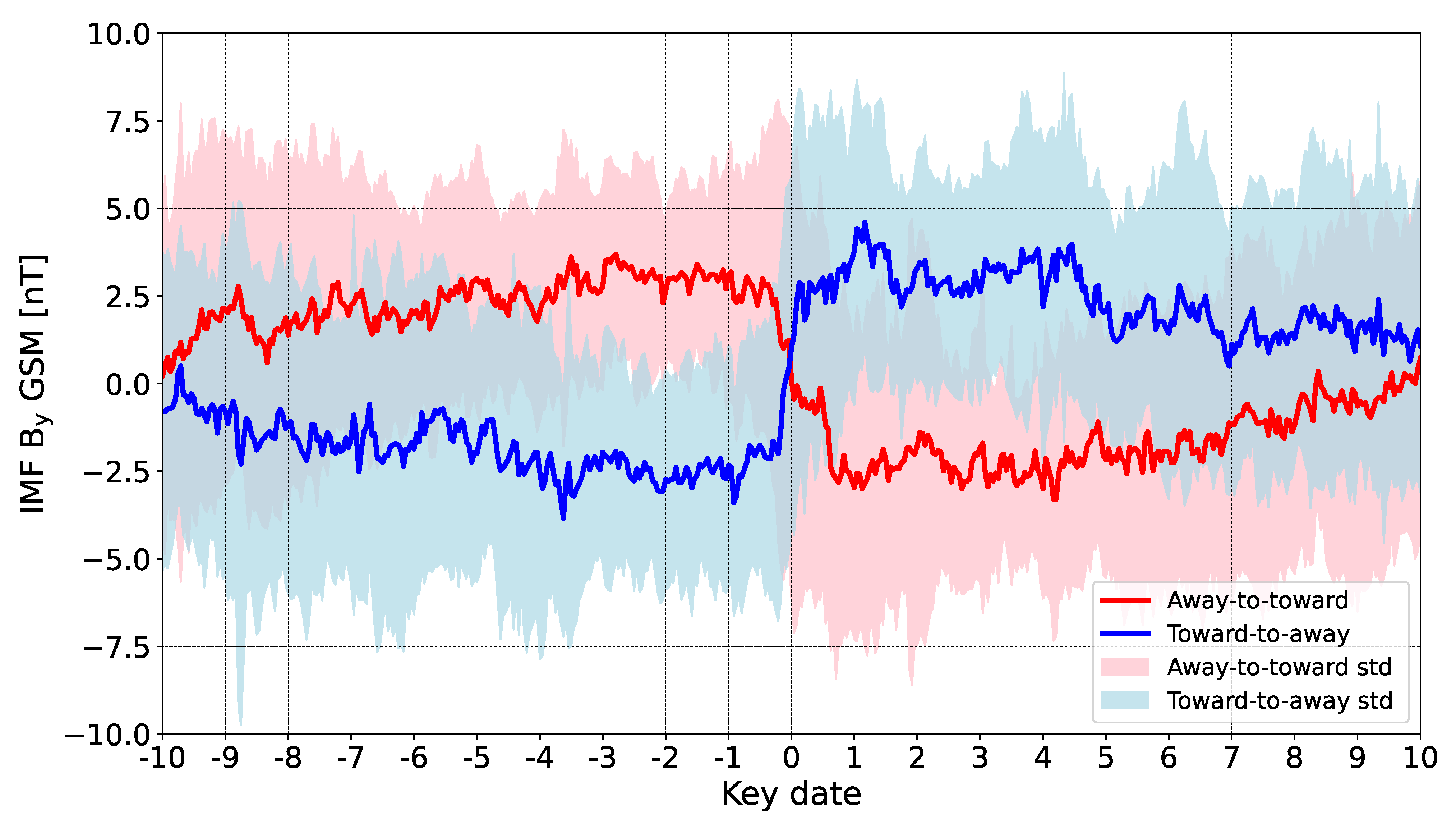
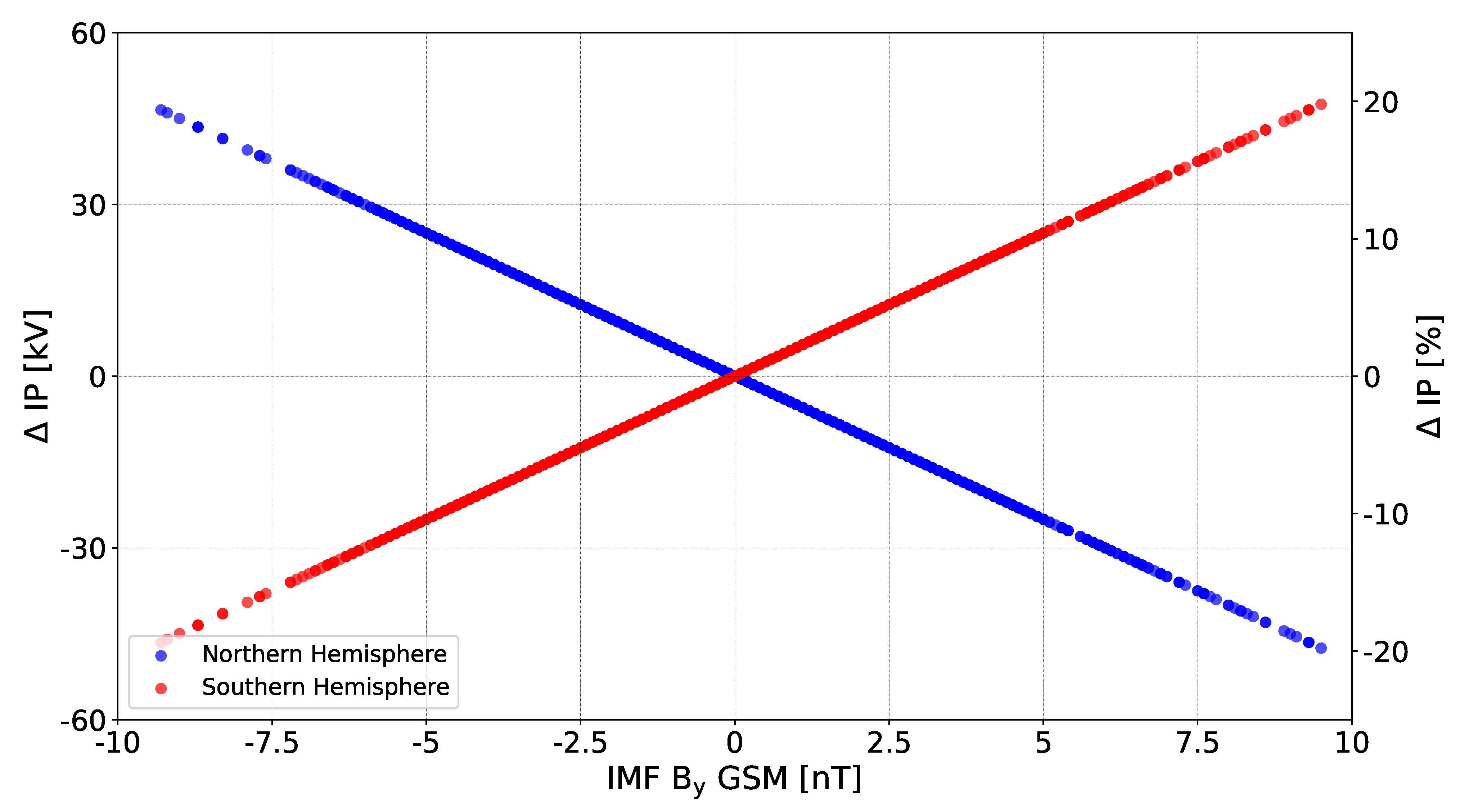
3.1. IMF B y and IMF B y -Associated Changes in Ionosphere-to-Ground (Ionospheric) Electric Potential (IP), Fair-Weather Current Density (J z ), and Cloud Microphysics

Here, we utilize daily-mean IMF B y in Geocentric Solar Magnetic (GSM) coordinates, obtained from the National Space Science Data Center (NSSDC) OMNIWeb database (https://omniweb.gsfc.nasa.gov, last accessed on 27 May 2022) for the interval 1999–2002. We analyze the solar maximum period (1999–2002), for which the effect is more readily apparent and the correlation between surface air pressure anomalies and IMF B y is large, as indicated in previous studies [5,7]. Moreover, for this period, statistically significant anomalies were found in both Arctic and Antarctic regions [5].
The East–West IMF B y has a well-established quasi-stable oscillation with 27 days of periodicity, caused by the Sun’s rotation. The state of IMF B y depends on the position of the heliospheric current sheet (HCS) relative to the Earth, which separates the regions of the magnetic field of opposite polarity. Reference [4] showed that IMF B y has a sharp polarity reversal at the time of HCS crossing.
Figure 1 illustrates the variation of IMF B y near the time of HCS crossing, utilizing the superposed epoch analysis for the 1999–2002 period.
The negative polarity of the IMF implies that the IMF lines are directed towards the Sun, while those directed towards the Earth have a positive polarity. The time of crossing the HCS is taken as zero dates. As the epochs, the data for ten days before and ten days after the date of the HCS crossing were selected. The epochs were chosen so that there were at least five days between neighboring HCS crossings. To have higher resolution, hourly-averaged IMF B y was taken here. Both, the exact time of the sector boundary transition and the polarity are taken from the database: (https://svalgaard.leif.org/research/sblist.txt, last accessed on 27 May 2022). In Figure 1, it is seen that the IMF B y becomes stronger near the HCS crossing date.
In this study, we employ the daily-mean IMF B y (i.e., daily variation of IMF B y is excluded and the IMF B y is constant throughout the day) since the meteorological response to changes of IMF B y might not be instant, which means that the relaxation time is longer than IMF B y resolution. This leads to an overlap of positive and negative effects, which is not favorable for obtaining the correct results. We also use a constant ionosphere-to-ground (ionospheric) electric potential (IP) of 250 kV, which is the observed daily-average value [42]. Using this value, we calculated the IP anomalies ( Δ IP) associated with IMF B y . These anomalies are shown in Figure 2.
According to previous studies, the IMF B y -associated anomalies in IP are inverted between hemispheres, i.e., Δ IP is positively correlated with IMF B y in the Southern Hemisphere, while they are negatively correlated in the Northern Hemisphere [5]. To calculate the anomalies, for simplicity, we applied ∼ ideal correlation between the changes in IP and IMF B y , but strictly following the magnitude of the anomalies estimated in the Weimer-2001 model [5]. Based on this, we believe that a change in the IMF B y by 1 nT causes a 2% change in IP. Thus, the obtained artificial anomalies in magnitude and sign are in good agreement with those shown in [5] for high magnetic latitudes.
Changes in the ionospheric potential lead to an equivalent change in J z by definition (since J z = IP/R, where R is the atmospheric column resistance), i.e., the magnitude of the change in J z is equal to the changes in IP under the action of IMF B y . Despite this, the geographic response of IP/J z on changes of IMF B y IP is still questionable. Moreover, the magnitude of J z -induced change in cloud microphysics remains uncertain.
Based on the results shown in Harrison et al. [23], we assume that IMF B y -associated electric effects and their impact on fair-weather cloud microphysics are equivalent, i.e., IP, J z , and cloud droplet coalescence rate are linearly dependent and have the same amount of change under the action of the IMF B y (see left y-axis in Figure 2).
Also in the SOCOLv3 model, we set compatible changes in the coalescence rate of liquid droplets and accretion of ice crystals under the action of IMF B y since in polar regions the liquid clouds might be rarely present.

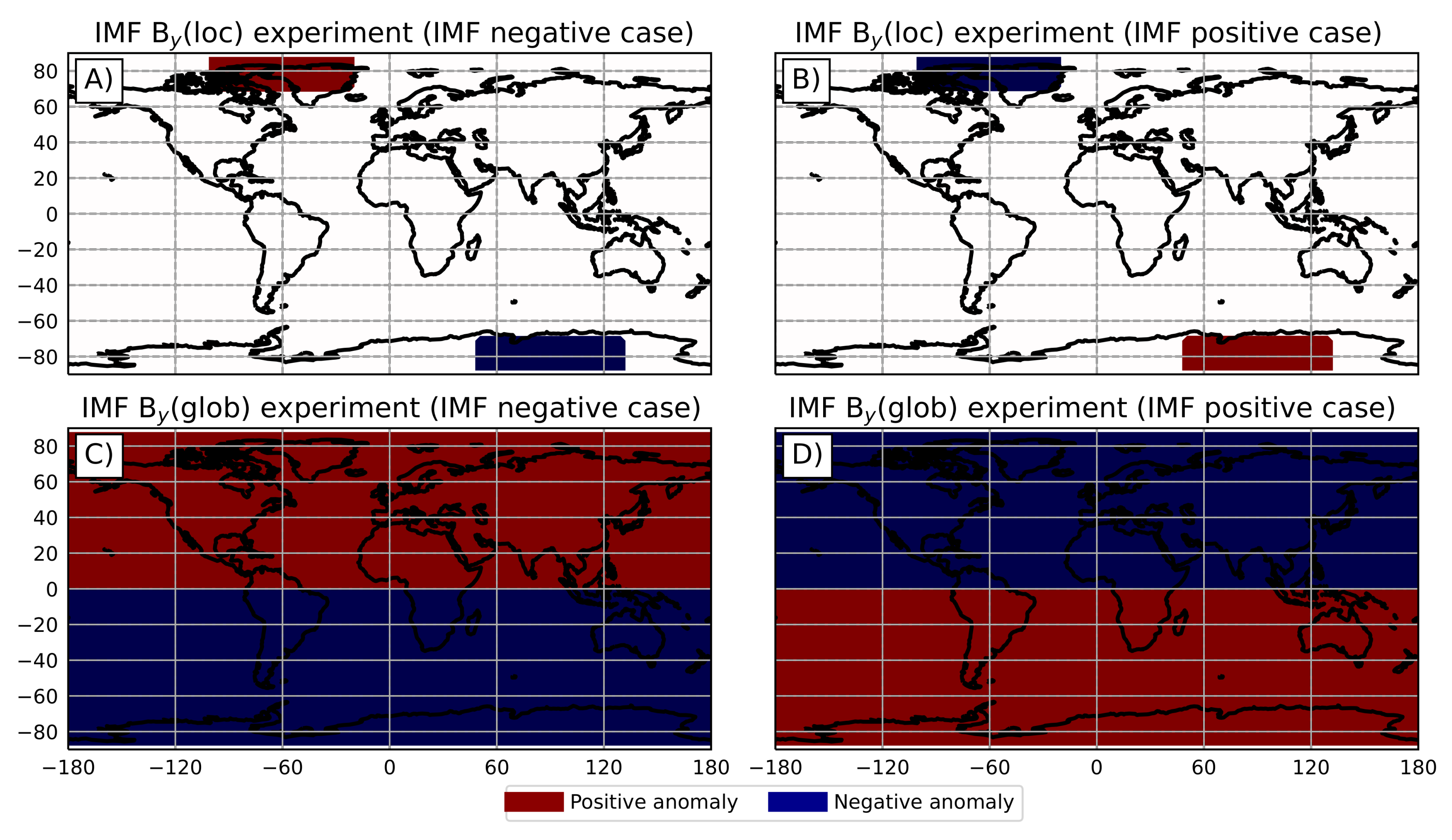
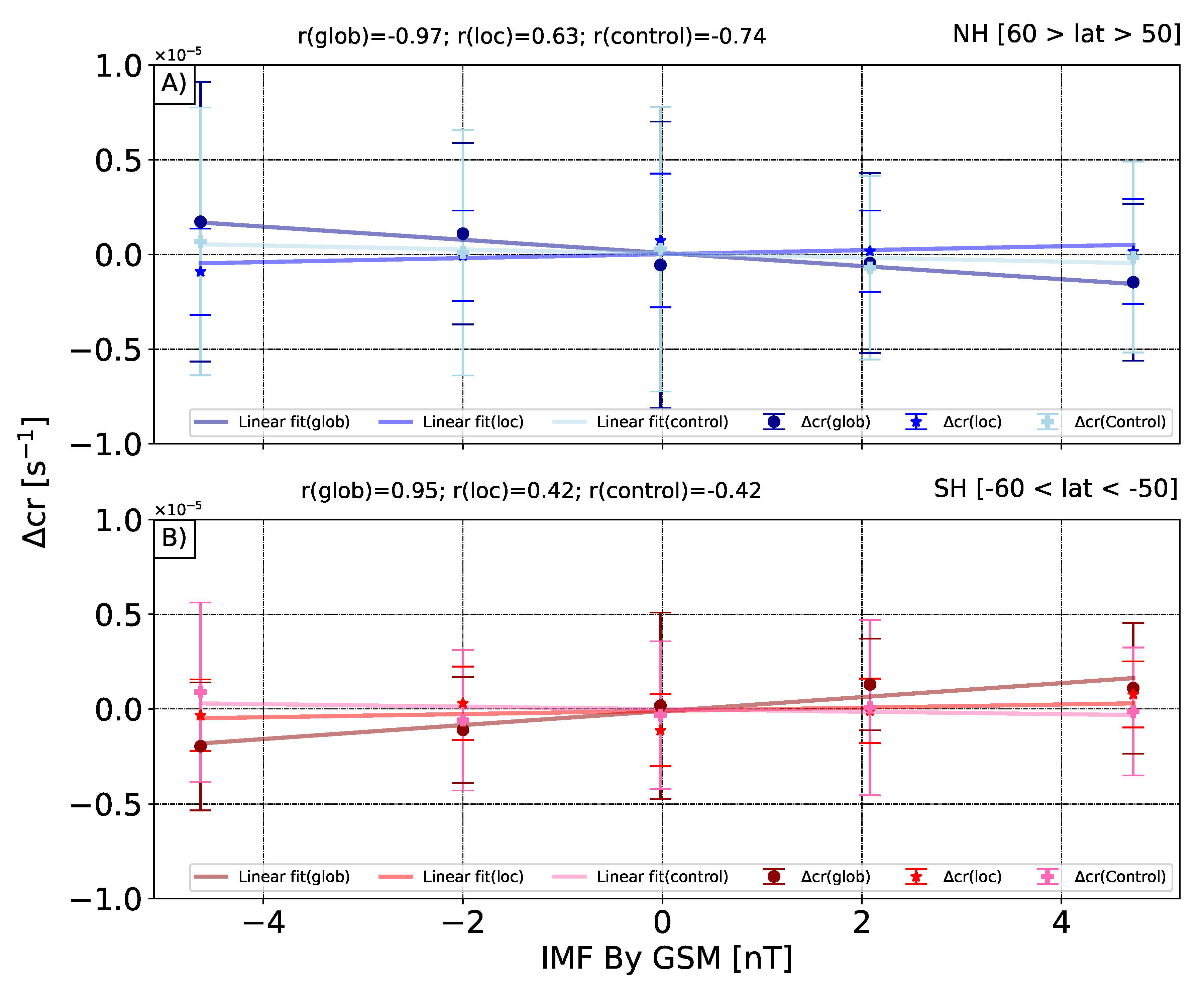
3.2. Model Experiments

In our research, to verify the GEC-cloud mechanism involved rate of droplet coalescence, we designed three numerical experiments using unperturbed (control) and perturbed conditions to calculate the response of surface pressure and temperature at two meters (2 m) on IMF B y fluctuation for the interval 1999–2002 (see Table 1).
In the control experiment, the IMF B y was not present and this experiment is used as a reference. In addition, we ran two experiments with perturbed conditions accounting for possible spatial distributions of B y -induced effects on J z : one where J z -imposed changes of cloud droplet coalescence are isolated within the region of IMF B y -induced changes in CPCP (see [7]) (hereinafter called IMF B y (loc) experiment); and another where J z -imposed changes of cloud droplet coalescence happen within the whole hemisphere (hereinafter called IMF B y (glob) experiment). J z effects are applied in both hemispheres, taking into account the hemispheric asymmetry of the IMF B y -induced effects due to the configuration of the magnetosphere-ionosphere current system [3]. The geography of applied anomalies is shown in Figure 3.
Each experiment consists of ten ensemble members, which are initialized with slightly varying initial conditions, i.e., a first-month small (0.1%) perturbation in the CO 2 concentration in order to describe the internal model variability and evaluate the statistical significance of the results. CO 2 is ordinarily used to create an ensemble in climate modeling, since even a slight change in its concentration affects the entire climate system, allowing different realizations of reality. Statistical significance was calculated using a Student t-test (https://github.com/scipy/scipy/blob/v1.8.0/scipy/stats/_stats_py.py#L5944-L6216, last accessed on 27 May 2022) applied between members of the ensemble experiment.
We use the methodology given in Lam et al. [7] to obtain surface pressure and 2 m temperature anomalies. From the obtained simulated results, we extract only the 12 UT data to exclude the diurnal cycle of meteorological parameters, as was proposed by Lam et al. [7].
Deseasonalization is applied as a subtraction of the mean 12 UT value for each “day of the year” for the whole 1999–2002 period (note that in Lam et al. [7], the seasonal cycle was approximated for the 1948–2011 interval). We use a seasonal model to decipher the seasonality. A description of the seasonal model is available here: (https://datalab.marine.rutgers.edu/2020/03/modeling-seasonal-data/, last accessed on 27 May 2022).
Since the period 1999–2002 was considered, there are only four values for each “day of the year”, so our seasonal model would be a bit noisy if we only used 1-day averages. To smooth the model a bit more, we use the 7-day rolling average. In addition, we estimated a trend using linear regression, which has also been excluded from the residuals.
After, the data residuals were sorted by five daily-mean IMF B y intervals: strongly positive (IMF B y ≥ 3 nT), moderately positive (3 nT > IMF B y ≥ 1 nT), near-neutral (1 nT > IMF B y > −1 nT), moderately negative (−1 nT ≥ IMF B y > −3 nT), strongly negative (IMF B y ≤ −3 nT). We calculated the mean of regularized residuals in each bin and extracted the mean for all IMF B y from each mean quantity. Despite the absence of IMF B y , we also applied the same procedure for the control experiment to determine the noise level in residuals. As was claimed in Tinsley [12], the statistical significance might be violated if the data for different seasons are mixed. However, Lam et al. [7] showed that for the interval 1999–2002 it is possible to obtain statistically significant anomalies even using the whole period and without applying seasonal analysis. Since we used the same methodology as used in Lam et al. [7], in this particular study we decided to analyze in the same manner, i.e., without dividing the data into seasons.
Figure 4 demonstrates an example of a linear regression between the IMF B y and anomalies in cloud droplet coalescence rate ( Δ cr) for middle latitudes [|60| > lat > |50|] from all three experiments.
The dependence of Δ cr and daily-mean IMF B y is visible, and the correlation for both hemispheres is ∼|1| from the B y (glob) experiment. In other experiments, a weak dependence and correlation were revealed. It is important to note here that the standard deviation is huge, spanning both negative and positive zones for each point (see error bars in Figure 4), which indicates a large internal variability of cloud microphysical parameters in the model.

4. Results

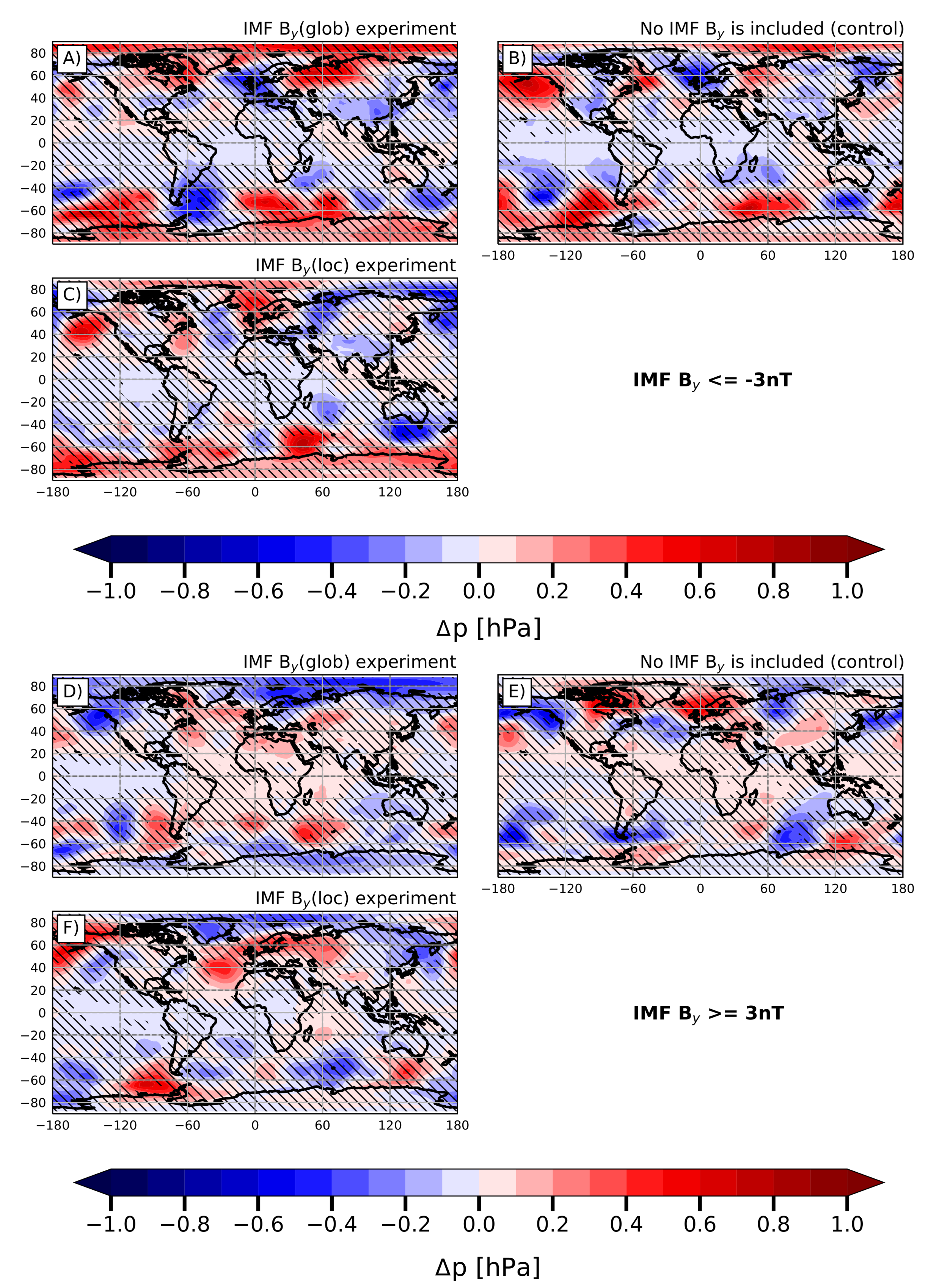
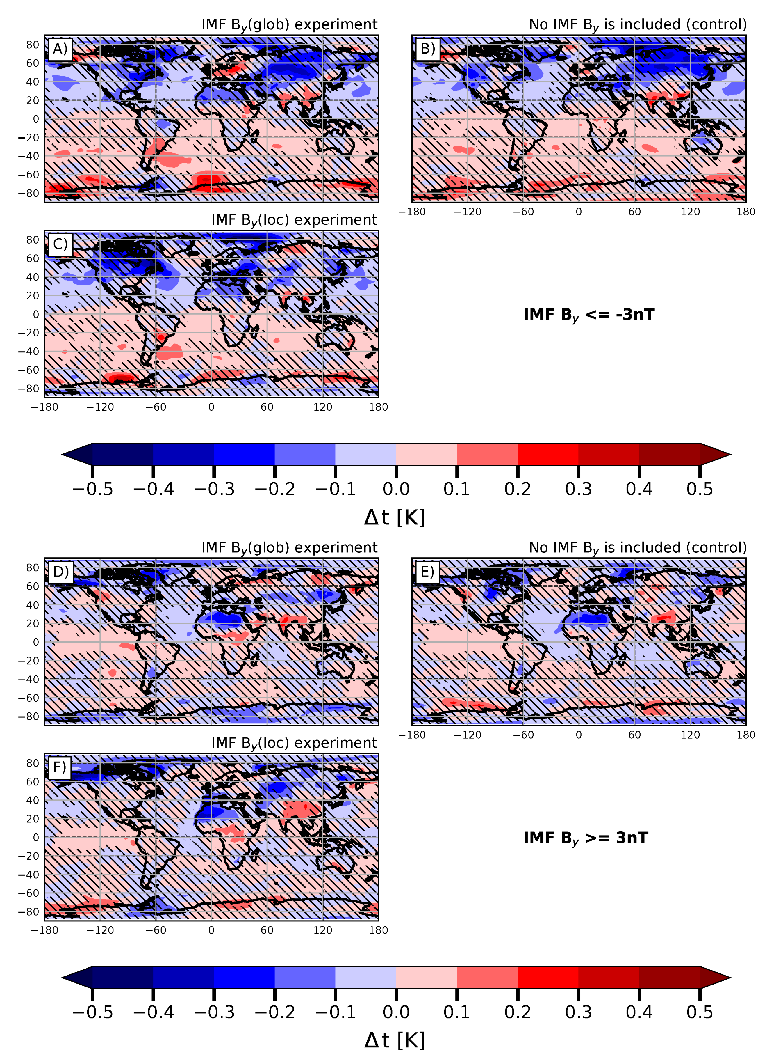
Geographical Distribution of Surface Air Pressure and 2 m Temperature Anomalies

Figure 5 illustrates global distributions of anomalies in surface air pressure ( Δ p) and 2 m air temperature ( Δ t) over the globe averaged for the 1999–2002 period.
Here, we show two extreme cases, namely when daily-mean IMF B y ≤ −3 nT and daily-mean IMF B y ≥ 3 nT. Spatial variations of Δ p with both negative and positive signs are seen over mid-to-high latitudes with an amplitude of ∼0.5–1 hPa in both IMF states. At high latitudes, there is a zonal alternation of negative and positive anomalies. Note that Δ p is not zero in all considered experiments, including the control experiment. In general, the difference in distributions of Δ p of perturbed (where IMF B y is included) experiments and control is small. Based on this, we suggest that obtained anomalies in surface air pressure cannot be explained by IMF B y fluctuation and might be caused by the internal model variability.
Similarly to Figure 5, Figure 6 demonstrates spatial distribution of Δ t. In all three experiments, Δ t is predominantly negative in the Northern Hemisphere and low positive in the Southern Hemisphere, showing a global magnitude of about −0.3 to 0.2 K. As it was for surface pressure, we compare Δ t from the control and both perturbed experiments. As a minor conclusion, we can say that IMF B y does not affect Δ t too, based on all three experiments, despite some minor spacial differences, which suggests that obtained Δ t might not originate from the IMF B y .
To support the above assumption, we also performed a linear regression between the daily average IMF B y and Δ p and Δ t, respectively, using the method presented in Burns et al. [5]. The result of the correlation test between Δ p and daily-mean IMF B y for high and mid-latitudes of both hemispheres is shown in Figure 7.
No dependence of the averaged Δ p and the IMF B y in a model similar to that presented in Burns et al. [5] was found. In fact, the standard deviation of Δ p between ensemble members is consistent with the magnitude of IMF B y -induced anomalies found in observations (see Burns et al. [5], Lam et al. [7]) even in the control experiment. No sign of hemispheric asymmetry associated with IMF B y is also revealed. This once again indicates that obtained anomalies in surface air pressure are caused not by IMF B y , but by other processes.
Figure 8 presents the linear regression between Δ t and daily-mean IMF B y . The magnitude of averaged Δ t is low. No correlation between IMF B y and Δ t for both hemispheres in high and mid-latitudes is also found.

5. Discussion

Here, we examine the meteorological response on interplanetary magnetic field B y component fluctuation, known as the Mansurov effect, to verify one of the hypotheses saying that this connection occurs via the global atmospheric electric circuit effects on cloud droplet coalescence rate. We performed a series of ten-member ensemble numerical experiments using the SOCOLv3 chemistry-climate model, endeavoring to find the effects of IMF B y on surface pressure and 2 m temperature, similar to those obtained earlier in the observations. In our study, we used the assumption that cloud droplet/ice coalescence rate and IP/J z -current response to IMF B y fluctuation have linear dependence. The results show that we cannot yet confirm the hypothesis that cloud droplet coalescence is the microphysical mechanism involved in the IMF B y -weather connection. General patterns of obtained anomalies in surface pressure Δ p and temperature Δ t are consistent between experiments with and without the IMF B y effect on the autoconversion rate. Linear regression showed no correlation between the considered meteorological parameters and IMF B y . The standard deviation of pressure and temperature residuals between ensemble members was found to be consistent with the reported IMF B y effects on surface meteorology given in previous studies [5,7]. The results were obtained using the same method. This indicates that even if the model showed the influence of IMF B y fluctuations on surface meteorology through cloud droplet coalescence, the internal model variability would overlap with it, preventing it from being properly estimated.
Here, we also need to highlight other important things that may affect the detection of the Mansurov effect in the simulation study and also discuss the assumptions that we used in our study and the perspectives of this study. Note that clouds could not be presented or are poorly presented on some days, decreasing our ability to detect anomalies properly. We would like to highlight that difficulties in simulating the Mansurov effect might also be generated by the poor accuracy of cloud microphysics in modern chemistry-climate models. It should be said again that to estimate the seasonal cycle, we used the same period for which we calculate the residuals (1999–2002), which may affect the accuracy. As was discussed in Tinsley [12], the mixing of seasons in the analysis might affect the statistical significance and decrease the signal in surface meteorology since it was shown that there is an increase in surface temperature and pressure due to increases in cloud opacity, for the typical polar stratiform clouds of optical thickness <1, which only occurs under winter conditions at high latitudes, and under summer conditions there are decreases in surface pressure and temperature with increases in cloud opacity. This is a possible reason for the underestimation of statistical significance in Edvartsen et al. [36]. However, in Lam et al. [7], Lam et al. [8], despite the analysis of the meteorological reanalysis data also being carried out without seasonal separation for the 1999–2002 period, the statistically significant meteorological response to IMF B y fluctuation was revealed using the less robust statistical method. In addition, the analyzing period is short, which may affect the accuracy, but it involves the solar maximum, and including the solar minimum in the analysis might decrease the signal/noise ratio. Note that for the correct identification of this effect, it is necessary to distinguish the signal from the noise associated with internal variability, as was shown by the control experiment. The linearity of the cloud microphysics response to IMF B y , i.e., sensitivity of cloud parameters to IMF B y -induced effects in GEC, is still questionable as the linearity assumption is only based on Harrison et al. [23]. Our study suggests that linear dependence does not allow for the detection of the signal for the hypothesis used here. Moreover, in our study, we assume that there is no decrease in Δ IP with decreasing latitude (in the IMF B y (glob) experiment, the influence is constant for the whole hemisphere) and ∼ ideal correlation between Δ IP and IMF B y , which did not help to reveal the impact of IMF B y on surface meteorology. In fact, as shown by [5], there is no ideal correlation between the anomalies in ionospheric potential IP and IMF B y ; the correlation is better near the magnetic pole (mlat > 80) and rapidly drops down together with the magnitude of anomalies with decreasing magnetic latitude. However, it remains unclear whether the IMF B y -related effect of GEC on cloud microphysics is localized at high latitudes or represented globally since both experiments showed no signal. Moreover, an interesting unconsidered effect is that the effect of the electric charges on cloud microphysics can compete with aerosols which can decrease the coalescence [28]. It is important also to consider the non-stationary behavior as well, as it is necessary to take into consideration the temporal autocorrelation for cyclic processes to study the Mansurov effect [36].
In general, the important point also is that the microphysical mechanism, in which the IMF B y -weather connection occurs through the increase of the autoconversion rate following the increase of J z , might be unfaithful. Therefore, the alternative mechanism, in which J z leads to an increase in cloud opacity due to the electro-anti-scavenging effect on CCN concentration, should also be tested in global climate models [10,11,12]. Hence, to study the electric effects on clouds, it is also worth considering advanced electric microphysics, including processes like electric-scavenging and electric-anti-scavenging [12,24,25,43,44]. However, the Advanced Aerosol Microphysics Module must also be enabled to perform the calculations, like the one included in the more advanced SOCOLv4 model [45].
Thus, more research efforts are needed to make it possible to model the Mansurov effect and to numerically support that the IMF B y -weather coupling occurs through the cloud microphysics.

6. Conclusions

The conclusions of our study are as follows:
  • We investigated the reaction of surface meteorology to IMF B y fluctuation using the chemistry-climate model SOCOLv3 to verify the mechanism in which this connection occurs through the altering of cloud droplet (ice) coalescence (accretion) rate under the action of the GEC.
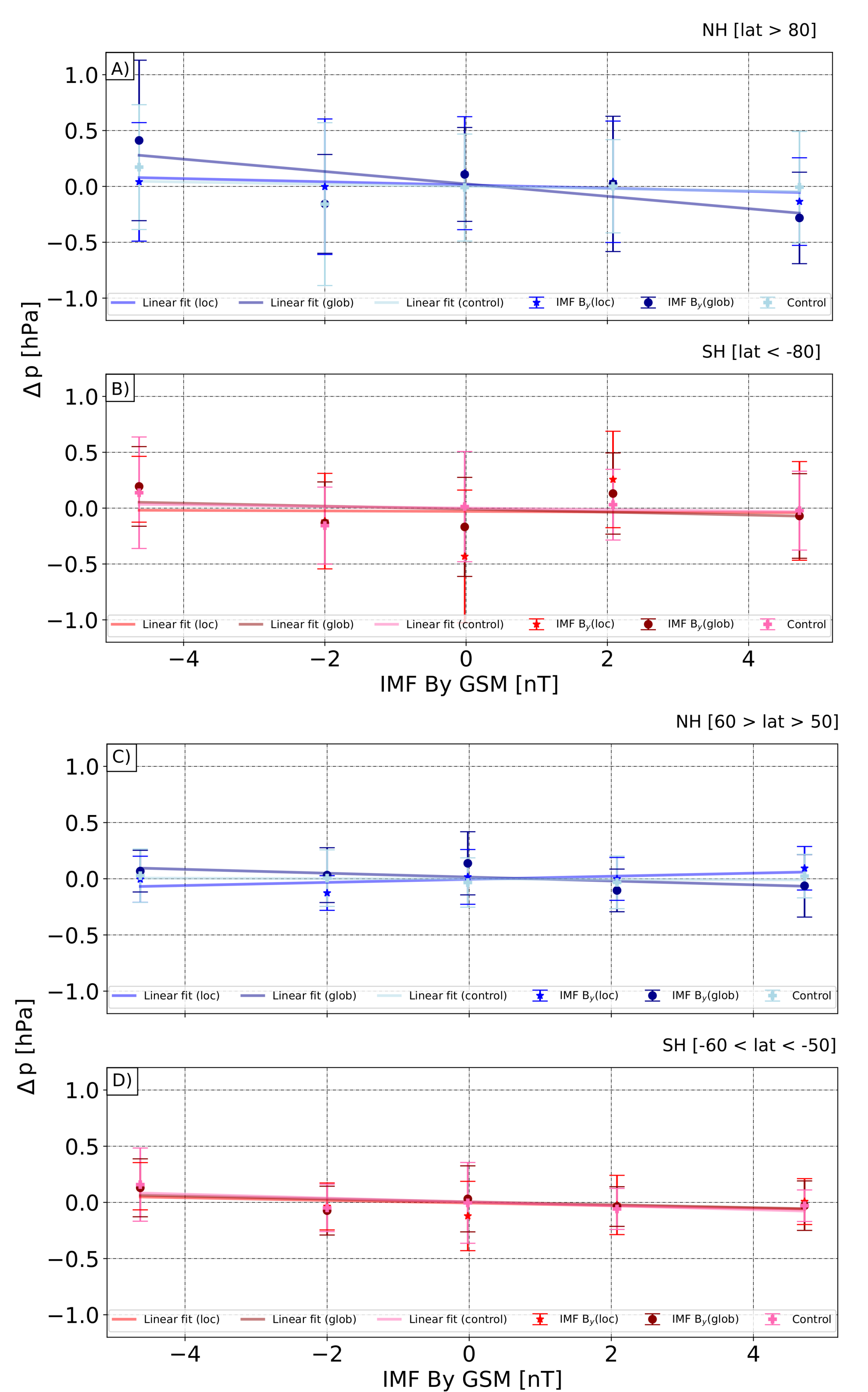
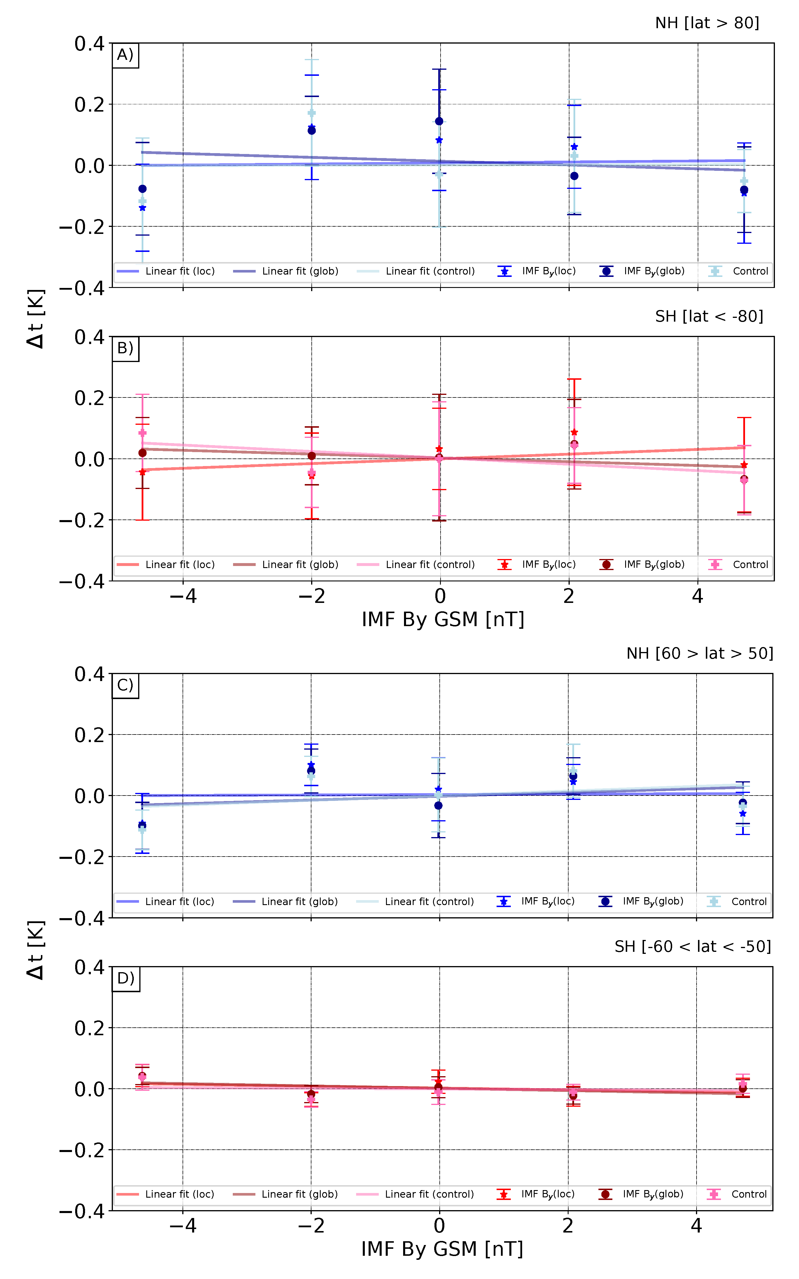
  • Model results and subsequent simple statistical analysis indicate that the IMF B y signal is not manifest itself in ground-level air pressure and temperature.
  • The internal model variability might interfere with revealing the IMF B y signal in surface meteorology, which shows the magnitude consistent with the magnitude of the control run.
  • The error in the mean of ensemble experiments is generally consistent with the magnitude of observed IMF B y -related anomalies.
  • The underlying unaccounted processes behind meteorological variability and remaining noise from the seasonal cycle or trend may also disrupt the distinguishing of the IMF B y -related anomalies in ground-level weather parameters.
  • The model results cannot confirm the hypothesis that the cloud droplet coalescence rate is the intermediate link for the IMF B y -weather coupling. Therefore, we only rule out the considered microphysical mechanism for the Mansurov effect, without weakening the likelihood of others or the observational evidence for the reality of the effect.

Author Contributions

A.K. prepared the original draft, run all simulations, and was mainly responsible for the visualization of the results. This research has been supervised and conceptualized by I.M. and E.R. All authors contributed to writing, analyzing, editing the manuscript, and discussing the results. All authors have read and agreed to the published version of the manuscript.

Funding

This research was funded by the Russian Foundation for Basic Research (RFFI) grant No. 19-35-90134. IM and AK were supported by the Russian Science Foundation (RNF) grant No. 20-67-46016. ER was supported by the Ministry of Science and Higher Education of the Russian Federation grant No. 075-15-2021-583 and the Russian Science Foundation (RNF) grant No. 21-17-00208.

Institutional Review Board Statement

Not applicable.

Informed Consent Statement

Not applicable.

Data Availability Statement

All data can be provided upon request.

Acknowledgments

We thank the Russian Foundation for Basic Research (RFFI) (project No. 19-35-90134) for Ph.D. student financial support of this study and the Russian Science Foundation (RNF) grant No. 20-67-46016, the SPbSU “Ozone Layer and Upper Atmosphere Research Laboratory” supported by the Ministry of Science and Higher Education of the Russian Federation under agreement 075-15-2021-583. IM and AK worked on the concept and writing the manuscript, analyzed the simulations, and did the visualization of results under the Russian Science Foundation (RNF) grant No. 20-67-46016. ER was partly supported by the Russian Science Foundation (RNF) (grant No. 21-17-00208). The authors also thank ETH’s High-Performance Computing Center (ID SIS) for the opportunity to use the Euler Linux cluster to conduct our numerical experiments and the Center for Climate Systems Modeling (C2SM) for their support.

Conflicts of Interest

The authors declare no conflict of interest.

Abbreviations

The following abbreviations are used in this manuscript:
IMFinterplanetary magnetic field
IMF B y dusk-to-dawn (B y ) component of IMF
GECglobal electric circuit
CPCPcross-polar-cap potential
CCNcloud condensation nuclei
CCMchemistry-climate model
GSMGeocentric Solar Magnetic
HCSheliospheric current sheet
MA-ECHAM5.4the Middle Atmosphere version of the European Center/Hamburg Model
version 5.4
CTMchemistry-transport model
MEZONModel for the Evaluation of oZONe Trends
NSSDCNational Space Science Data Center
IPionospheric (ionosphere-to-ground) potential

References

  1. Mansurov, S.M.; Mansurova, L.G.; Mansurov, G.S.; Mikhnevich, V.V.; Visotskii, A.M. North-south asymmetry of geomagnetic and tropospheric events. J. Atmos. Terr. Phys. 1974, 36, 1957. [Google Scholar] [CrossRef]
  2. Page, D.E. The interplanetary magnetic field and sea level polar atmospheric pressure. Workshop Mech. Tropospheric Eff. Sol. Var.-Quasi-Bienn. Oscil. 1993, 98, 227. [Google Scholar]
  3. Tinsley, B.A.; Heelis, R.A. Correlations of atmospheric dynamics with solar activity evidence for a connection via the solar wind, atmospheric electricity, and cloud microphysics. J. Geophys. Res. (Atmos.) 1993, 98, 10375–10384. [Google Scholar] [CrossRef] [Green Version]
  4. Burns, G.B.; Tinsley, B.A.; Frank-Kamenetsky, A.V.; Bering, E.A. Interplanetary magnetic field and atmospheric electric circuit influences on ground-level pressure at Vostok. J. Geophys. Res. (Atmos.) 2007, 112, D04103. [Google Scholar] [CrossRef] [Green Version]
  5. Burns, G.B.; Tinsley, B.A.; French, W.J.R.; Troshichev, O.A.; Frank-Kamenetsky, A.V. Atmospheric circuit influences on ground-level pressure in the Antarctic and Arctic. J. Geophys. Res. (Atmos.) 2008, 113, D15112. [Google Scholar] [CrossRef] [Green Version]
  6. Tinsley, B.A. The global atmospheric electric circuit and its effects on cloud microphysics. Rep. Prog. Phys. 2008, 71, 066801. [Google Scholar] [CrossRef]
  7. Lam, M.M.; Chisham, G.; Freeman, M.P. The interplanetary magnetic field influences mid-latitude surface atmospheric pressure. Environ. Res. Lett. 2013, 8, 045001. [Google Scholar] [CrossRef] [Green Version]
  8. Lam, M.M.; Chisham, G.; Freeman, M.P. Solar wind-driven geopotential height anomalies originate in the Antarctic lower troposphere. Geophys. Res. Lett. 2014, 41, 6509–6514. [Google Scholar] [CrossRef] [Green Version]
  9. Freeman, M.P.; Lam, M.M. Regional, seasonal, and inter-annual variations of Antarctic and sub-Antarctic temperature anomalies related to the Mansurov effect. Environ. Res. Commun. 2019, 1, 111007. [Google Scholar] [CrossRef]
  10. Frederick, J.E.; Tinsley, B.A.; Zhou, L. Relationships between the solar wind magnetic field and ground-level longwave irradiance at high northern latitudes. J. Atmos. Sol.-Terr. Phys. 2019, 193, 105063. [Google Scholar] [CrossRef]
  11. Tinsley, B.A.; Zhou, L.; Wang, L.; Zhang, L. Seasonal and Solar Wind Sector Duration Influences on the Correlation of High Latitude Clouds with Ionospheric Potential. J. Geophys. Res. (Atmos.) 2021, 126, e34201. [Google Scholar] [CrossRef]
  12. Tinsley, B.A. Uncertainties in Evaluating Global Electric Circuit Interactions With Atmospheric Clouds and Aerosols, and Consequences for Radiation and Dynamics. J. Geophys. Res. (Atmos.) 2022, 127, e35954. [Google Scholar] [CrossRef]
  13. Hairston, M.R.; Heelis, R.A. Model of the high-latitude ionospheric convection pattern during southward interplanetary magnetic field using DE 2 data. J. Geophys. Res. (Atmos.) 1990, 95, 2333–2343. [Google Scholar] [CrossRef]
  14. Weimer, D.R. A flexible, IMF dependent model of high-latitude electric potentials having “Space Weather” applications. Geophys. Res. Lett. 1996, 23, 2549–2552. [Google Scholar] [CrossRef]
  15. Weimer, D.R. An improved model of ionospheric electric potentials including substorm perturbations and application to the Geospace Environment Modeling November 24, 1996, event. J. Geophys. Res. (Atmos.) 2001, 106, 407–416. [Google Scholar] [CrossRef]
  16. Pettigrew, E.D.; Shepherd, S.G.; Ruohoniemi, J.M. Climatological patterns of high-latitude convection in the Northern and Southern Hemispheres: Dipole tilt dependencies and interhemispheric comparisons. J. Geophys. Res. (Space Phys.) 2010, 115, A07305. [Google Scholar] [CrossRef] [Green Version]
  17. Cowley, S.W.H.; Lockwood, M. Excitation and decay of solar wind-driven flows in the magnetosphere-ionosphere system. Ann. Geophys. 1992, 10, 103–115. [Google Scholar]
  18. Lucas, G.M.; Baumgaertner, A.J.G.; Thayer, J.P. A global electric circuit model within a community climate model. J. Geophys. Res. (Atmos.) 2015, 120, 12054–12066. [Google Scholar] [CrossRef]
  19. Rycroft, M.J.; Nicoll, K.A.; Aplin, K.L.; Giles Harrison, R. Recent advances in global electric circuit coupling between the space environment and the troposphere. J. Atmos. Sol.-Terr. Phys. 2012, 90, 198–211. [Google Scholar] [CrossRef] [Green Version]
  20. Wilson, C.T.R. A Theory of Thundercloud Electricity. Proc. R. Soc. London. Ser. A Math. Phys. Sci. 1956, 236, 297–317. [Google Scholar]
  21. Zhou, L.; Tinsley, B.A. Production of space charge at the boundaries of layer clouds. J. Geophys. Res. (Atmos.) 2007, 112, D11203. [Google Scholar] [CrossRef] [Green Version]
  22. Nicoll, K.A. Measurements of Atmospheric Electricity Aloft. Surv. Geophys. 2012, 33, 991–1057. [Google Scholar] [CrossRef]
  23. Harrison, R.G.; Nicoll, K.A.; Ambaum, M.H.P. On the microphysical effects of observed cloud edge charging. Q. J. R. Meteorol. Soc. 2015, 141, 2690–2699. [Google Scholar] [CrossRef]
  24. Tinsley, B.A.; Deen, G.W. Apparent tropospheric response to MeV-GeV particle flux variations: A connection via electrofreezing of supercooled water in high-level clouds? J. Geophys. Res. (Atmos.) 1991, 96, 22283–22296. [Google Scholar] [CrossRef] [Green Version]
  25. Zhou, L.; Tinsley, B.A.; Wang, L.; Burns, G. The zonal-mean and regional tropospheric pressure responses to changes in ionospheric potential. J. Atmos. Sol.-Terr. Phys. 2018, 171, 111–118. [Google Scholar] [CrossRef]
  26. Harrison, R.G.; Lockwood, M. Rapid indirect solar responses observed in the lower atmosphere. Proc. R. Soc. Lond. Ser. A 2020, 476, 20200164. [Google Scholar] [CrossRef]
  27. Baumgaertner, A.J.G.; Lucas, G.M.; Thayer, J.P.; Mallios, S.A. On the role of clouds in the fair weather part of the global electric circuit. Atmos. Chem. Phys. 2014, 14, 8599–8610. [Google Scholar] [CrossRef] [Green Version]
  28. Guo, S.; Xue, H. The enhancement of droplet collision by electric charges and atmospheric electric fields. Atmos. Chem. Phys. 2021, 21, 69–85. [Google Scholar] [CrossRef]
  29. Lachlan-Cope, T. Antarctic clouds. Natl. Inst. Polar Res. Mem. 2010, 29, 150–158. [Google Scholar] [CrossRef]
  30. Bromwich, D.H.; Nicolas, J.P.; Hines, K.M.; Kay, J.E.; Key, E.L.; Lazzara, M.A.; Lubin, D.; McFarquhar, G.M.; Gorodetskaya, I.V.; Grosvenor, D.P.; et al. Tropospheric clouds in Antarctica. Rev. Geophys. 2012, 50, RG1004. [Google Scholar] [CrossRef] [Green Version]
  31. Lam, M.M.; Freeman, M.P.; Chisham, G. IMF-driven change to the Antarctic tropospheric temperature due to the global atmospheric electric circuit. J. Atmos. Sol.-Terr. Phys. 2018, 180, 148–152. [Google Scholar] [CrossRef] [Green Version]
  32. Mareev, E.A.; Volodin, E.M. Variation of the global electric circuit and Ionospheric potential in a general circulation model. Geophys. Res. Lett. 2014, 41, 9009–9016. [Google Scholar] [CrossRef]
  33. Karagodin, A.; Rozanov, E.; Mareev, E.; Mironova, I.; Volodin, E.; Golubenko, K. The representation of ionospheric potential in the global chemistry-climate model SOCOL. Sci. Total. Environ. 2019, 697, 134172. [Google Scholar] [CrossRef] [PubMed]
  34. Golubenko, K.; Rozanov, E.; Mironova, I.; Karagodin, A.; Usoskin, I. Natural Sources of Ionization and Their Impact on Atmospheric Electricity. Geophys. Res. Lett. 2020, 47, e88619. [Google Scholar] [CrossRef]
  35. Karagodin, A.; Mironova, I.; Rozanov, E. Sensitivity of Surface Meteorology to Changes in Cloud Microphysics Associated with IMF By. In Problems of Geocosmos–2020; Springer Proceedings in Earth and Environmental Sciences; Springer Nature: Cham, Switzerland, 2022; pp. 413–420. [Google Scholar] [CrossRef]
  36. Edvartsen, J.; Maliniemi, V.; Tyssøy, H.N.; Asikainen, T.; Hatch, S.M. The Mansurov effect: Statistical significance and the role of autocorrelation. J. Space Weather Space Clim. 2022, 12, 11. [Google Scholar] [CrossRef]
  37. Stenke, A.; Schraner, M.; Rozanov, E.; Egorova, T.; Luo, B.; Peter, T. The SOCOL version 3.0 chemistry-climate model: Description, evaluation, and implications from an advanced transport algorithm. Geosci. Model Dev. 2013, 6, 1407–1427. [Google Scholar] [CrossRef] [Green Version]
  38. Manzini, E.; Giorgetta, M.A.; Esch, M.; Kornblueh, L.; Roeckner, E. The Influence of Sea Surface Temperatures on the Northern Winter Stratosphere: Ensemble Simulations with the MAECHAM5 Model. J. Clim. 2006, 19, 3863. [Google Scholar] [CrossRef]
  39. Rozanov, E.V.; Zubov, V.A.; Schlesinger, M.E.; Yang, F.; Andronova, N.G. The UIUC three-dimensional stratospheric chemical transport model: Description and evaluation of the simulated source gases and ozone. J. Geophys. Res. (Atmos.) 1999, 104, 11755–11781. [Google Scholar] [CrossRef]
  40. Egorova, T.; Rozanov, E.; Zubov, V.; Karol, I. Model for investigating ozone trends (MEZON). Izv.-Atmos. Ocean. Phys. 2003, 39, 277–292. [Google Scholar]
  41. Lohmann, U.; Roeckner, E. Design and performance of a new cloud microphysics scheme developed for the ECHAM general circulation model. Clim. Dyn. 1996, 12, 557–572. [Google Scholar] [CrossRef]
  42. Markson, R. Aircraft measurements of the atmospheric electrical global circuit during the period 1971–1984. J. Geophys. Res. (Atmos.) 1985, 90, 5967–5977. [Google Scholar] [CrossRef]
  43. Tinsley, B.A.; Zhou, L. Parameterization of aerosol scavenging due to atmospheric ionization. J. Geophys. Res. (Atmos.) 2015, 120, 8389–8410. [Google Scholar] [CrossRef]
  44. Zhang, L.; Tinsley, B.; Zhou, L. Parameterization of In-Cloud Aerosol Scavenging Due to Atmospheric Ionization: Part 4. Effects of Varying Altitude. J. Geophys. Res. (Atmos.) 2019, 124, 13105–13126. [Google Scholar] [CrossRef]
  45. Sukhodolov, T.; Egorova, T.; Stenke, A.; Ball, W.T.; Brodowsky, C.; Chiodo, G.; Feinberg, A.; Friedel, M.; Karagodin-Doyennel, A.; Peter, T.; et al. Atmosphere-ocean-aerosol-chemistry-climate model SOCOLv4.0: Description and evaluation. Geosci. Model Dev. 2021, 14, 5525–5560. [Google Scholar] [CrossRef]
Figure 1. Superposed epoch analysis of the IMF B y around the HCS crossing for the period 1999–2002. Blue line: toward-to-away IMF B y change; Red line: away-to-toward IMF B y change. Shadings represent standard errors in the means.
Atmosphere 13 00881 g001
Figure 2. The estimated IMF B y -associated perturbations in ionosphere-to-ground potential for the 1999–2002 period. Percentage anomalies (left y-axis) are calculated from daily average IP (250 kV).
Atmosphere 13 00881 g002
Figure 3. The geography of IMF B y -associated anomalies applied in IP, J z , and cloud droplet coalescence rate. Panels A and B: anomalies used in IMF B y (loc) experiment for negative (A) and positive (B) IMF B y state; panels C and D: anomalies used in IMF B y (glob) experiment for negative (C) and positive (D) IMF B y state. Red region: positive anomaly; blue region: negative anomaly.
Atmosphere 13 00881 g003
Figure 4. Ensemble-mean linear regression of Δ cr and daily-mean IMF B y for the 1999–2002 period for mid-latitudes. Data were binned and averaged for five daily-mean IMF B y intervals (see experiment description). Dark blue and dark red: B y (glob) experiment; blue and red: B y (loc) experiment; light blue and pink: the control experiment. Panel (A): Δ t for Northern Hemisphere mid-latitudes (60 > lat > 50); panel (B): Δ t for Southern Hemisphere mid-latitudes (−60 < lat < −50). Error bars are plus/minus standard error in the mean of Δ cr between ensemble members. r represents Pearson’s correlation coefficient.
Atmosphere 13 00881 g004
Figure 5. Ensemble-mean geographical distribution of Δ p averaged for the interval 1999–2002. Panels A, B, and C: Δ p averaged over days with daily-mean IMF B y ≤ −3 nT from B y (glob) (A), control (B), and B y (loc) (C) experiments; panels D, E, and F: Δ p averaged over days with daily-mean IMF B y ≥ 3 nT from B y (glob) (D), control (E), and B y (loc) (F) experiments. Hatches represent a probability of Δ p less than 95%.
Atmosphere 13 00881 g005
Figure 6. Ensemble-mean geographical distribution of Δ t averaged for the interval 1999–2002. Panels A, B, and C: Δ t averaged over days with daily-mean IMF B y ≤ −3 nT from B y (glob) (A), control (B), and B y (loc) (C) experiments; panels D, E, and F: Δ t averaged over days with daily-mean IMF B y ≥ 3 nT from B y (glob) (D), control (E), and B y (loc) (F) experiments. Hatches represent the probability of anomalies less than 95%.
Atmosphere 13 00881 g006
Figure 7. Ensemble-mean linear regression of Δ p and daily-mean IMF B y for the 1999–2002 period. Data were binned and averaged for five daily-mean IMF B y intervals (see experiment description). Blue and red: B y (loc) experiment; dark blue and dark red: B y (glob) experiment; light blue and pink: the control experiment. Panels A and B: Δ p for Northern Hemisphere (A: lat > 80) and mid-latitudes (B: 60 > lat > 50); panels C and D: Δ p for Southern Hemisphere (C: lat > 80) and mid-latitudes (D: −60 < lat < −50). Error bars are plus/minus standard error in the mean of Δ p between ensemble members.
Atmosphere 13 00881 g007
Figure 8. Ensemble-mean linear regression of Δ t and daily-mean IMF B y for the 1999–2002 period. Data were binned and averaged for five daily-mean IMF B y intervals (see experiment description). Blue and red: B y (loc) experiment; dark blue and dark red: B y (glob) experiment; light blue and pink: the control experiment. Panels A and B: Δ t for Northern Hemisphere (A: lat > 80) and mid-latitudes (B: 60 > lat > 50); panels C and D: Δ t for Southern Hemisphere (C: lat > 80) and mid-latitudes (D: −60 < lat < −50). Error bars are plus/minus standard error in the mean of Δ t between ensemble members.
Atmosphere 13 00881 g008
Table 1. The setup of model experiments.
Name of ExperimentExperiment DescriptionPeriod of Simulation
ControlNo IMF B y is used (10 ensemble members)1999–2002
B y (loc) experimentIMF B y contributes locally near the magnetic pole (|70| < mlat) (10 ensemble members)1999–2002
B y (glob) experimentIMF B y contributes globally within the entire hemisphere (10 ensemble members)1999–2002
Publisher’s Note: MDPI stays neutral with regard to jurisdictional claims in published maps and institutional affiliations.

