
Air Quality Impact Assessment of a Waste-to-Energy Plant: Modelling Results vs. Monitored Data


Abstract
:1. Introduction
2. Materials and Methods
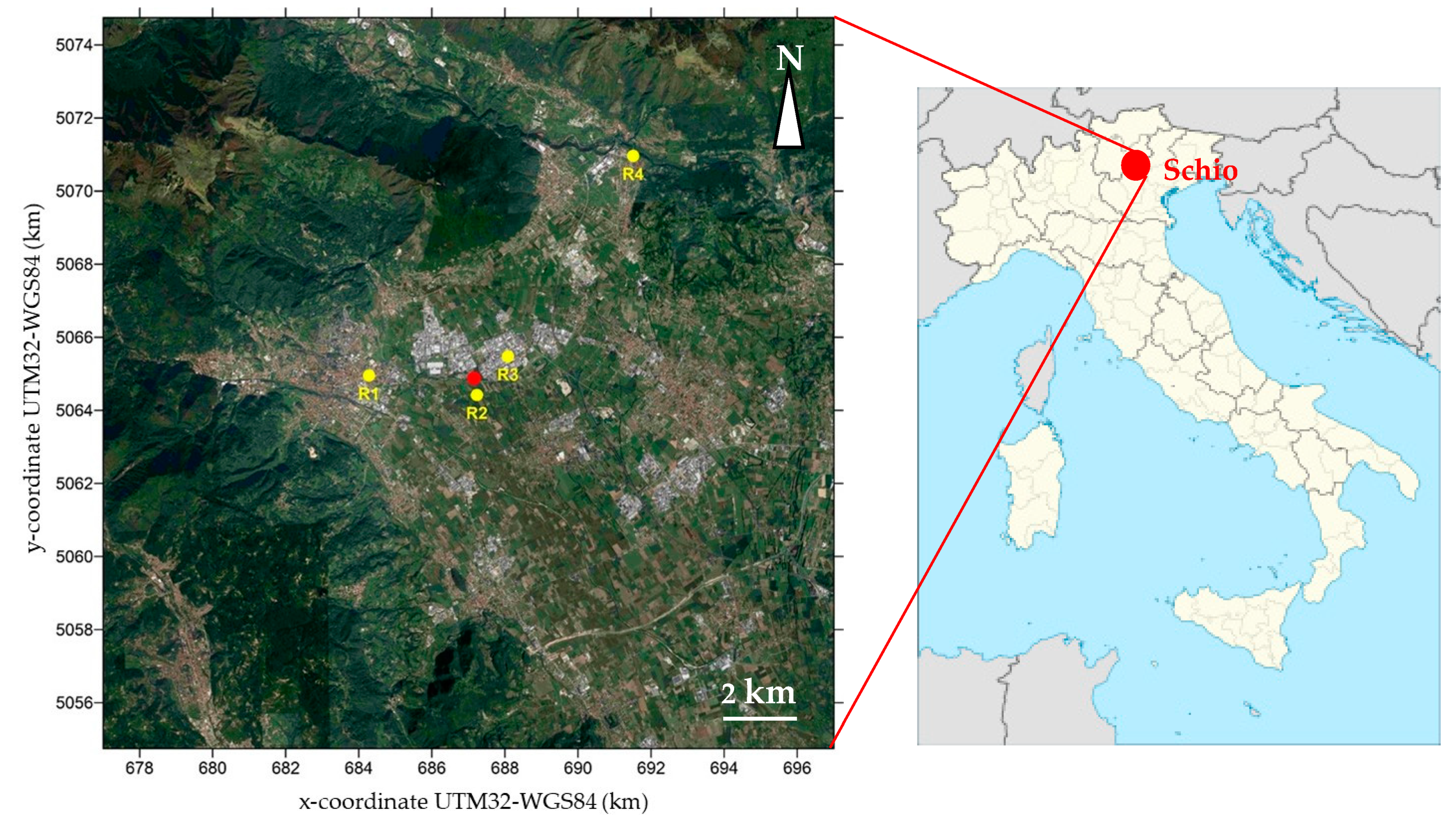
2.1. Study Area
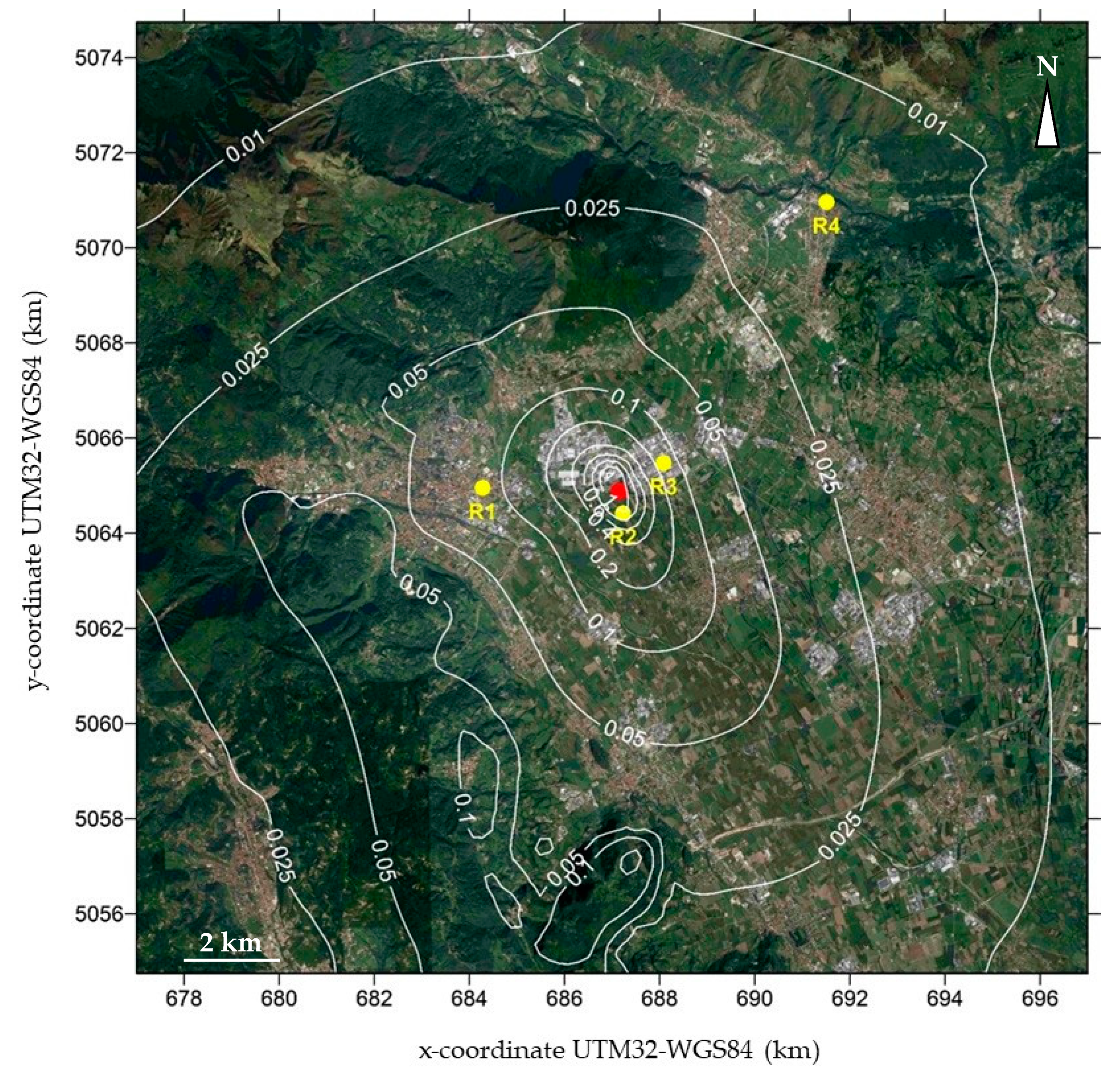
2.2. Modelling System
2.2.1. Emission Data
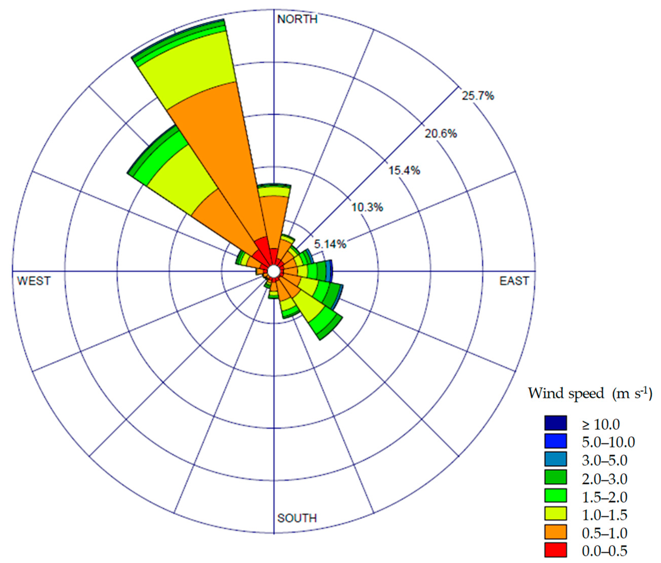
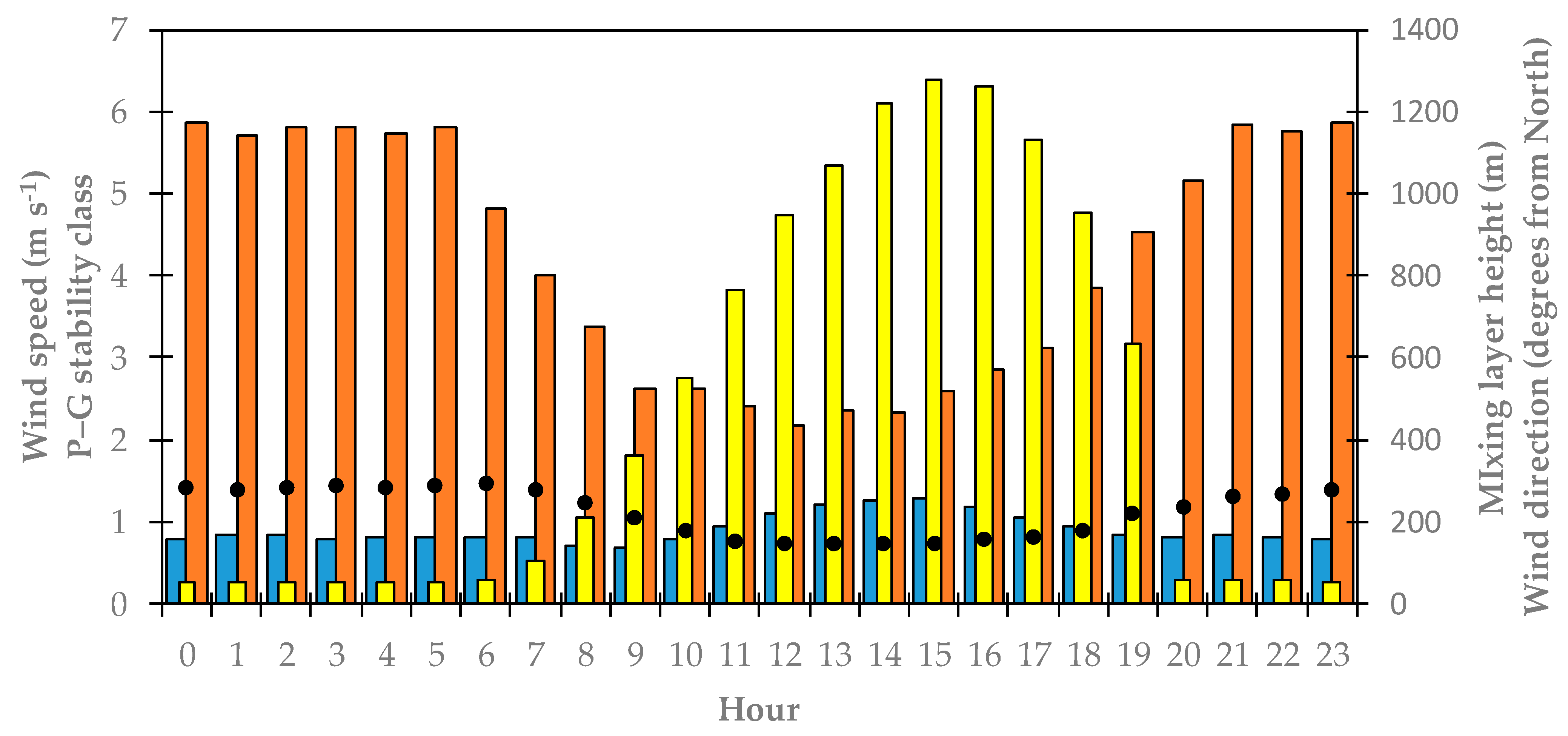
2.2.2. Meteorological Data
- -
- Wind speed was substantially uniform throughout the day, usually below 1 m s−1 but with a slight increase in the afternoon;
- -
- Winds were usually aligned in the NNW-SSE direction, blowing towards the plain during nighttime, early morning, and early evening hours and towards the mountain during daytime hours;
- -
- Conditions of neutral and stable atmosphere occurred from the evening to the early hours of the morning, followed by a progressive increase in instability until mid-afternoon;
- -
- The evolution of the height of the mixed layer followed a temporal profile anticorrelated with atmospheric stability, with shallow values in the orders of 50 m in the evening and night hours, gradually increasing in the morning up to maximum values of the orders of 1000–1200 m in the hours before sunset.
2.3. Air Quality Data
3. Results
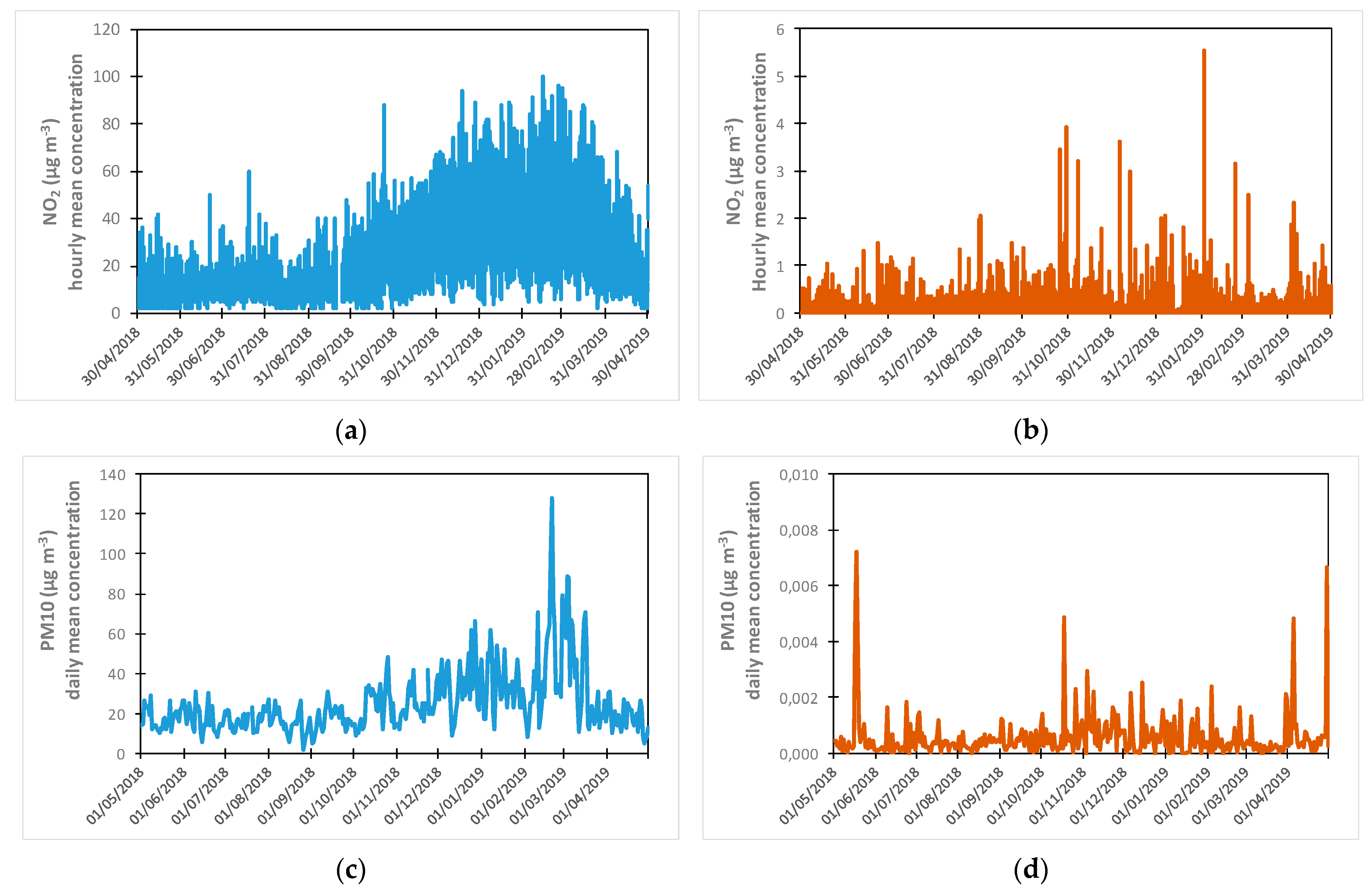
3.1. Air Quality Monitoring Site R1
3.2. Monitoring Sites R2, R3, and R4
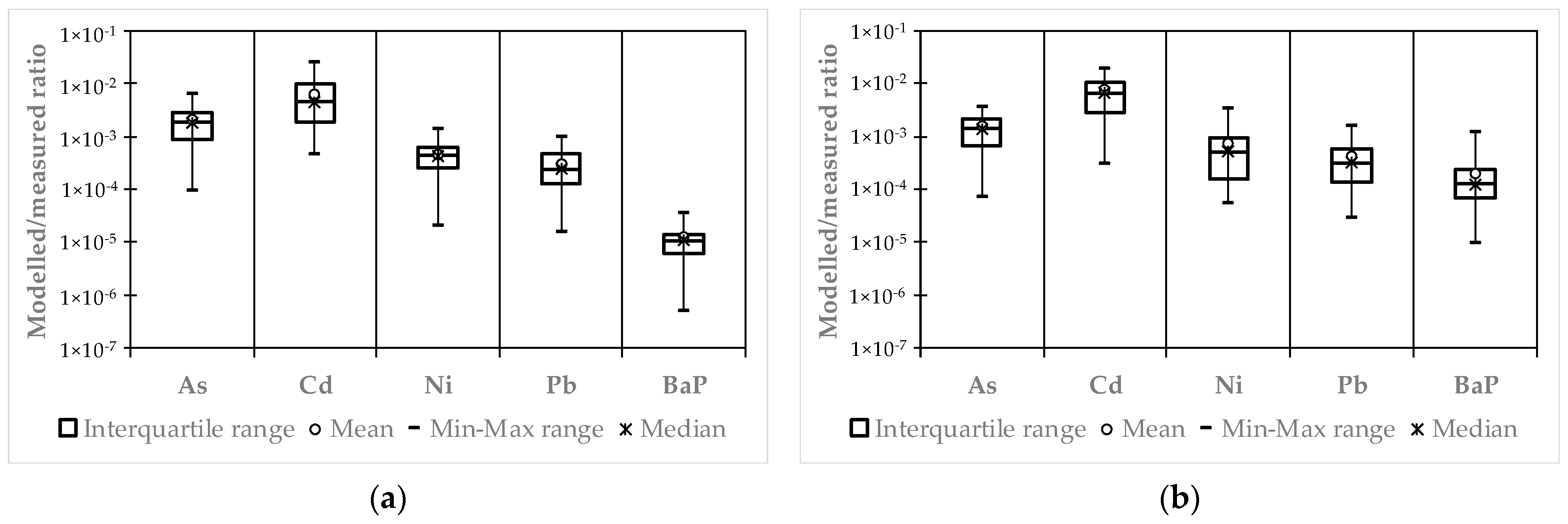
3.2.1. Toxic Elements and Benzo(a)pyrene
3.2.2. PCDD/F
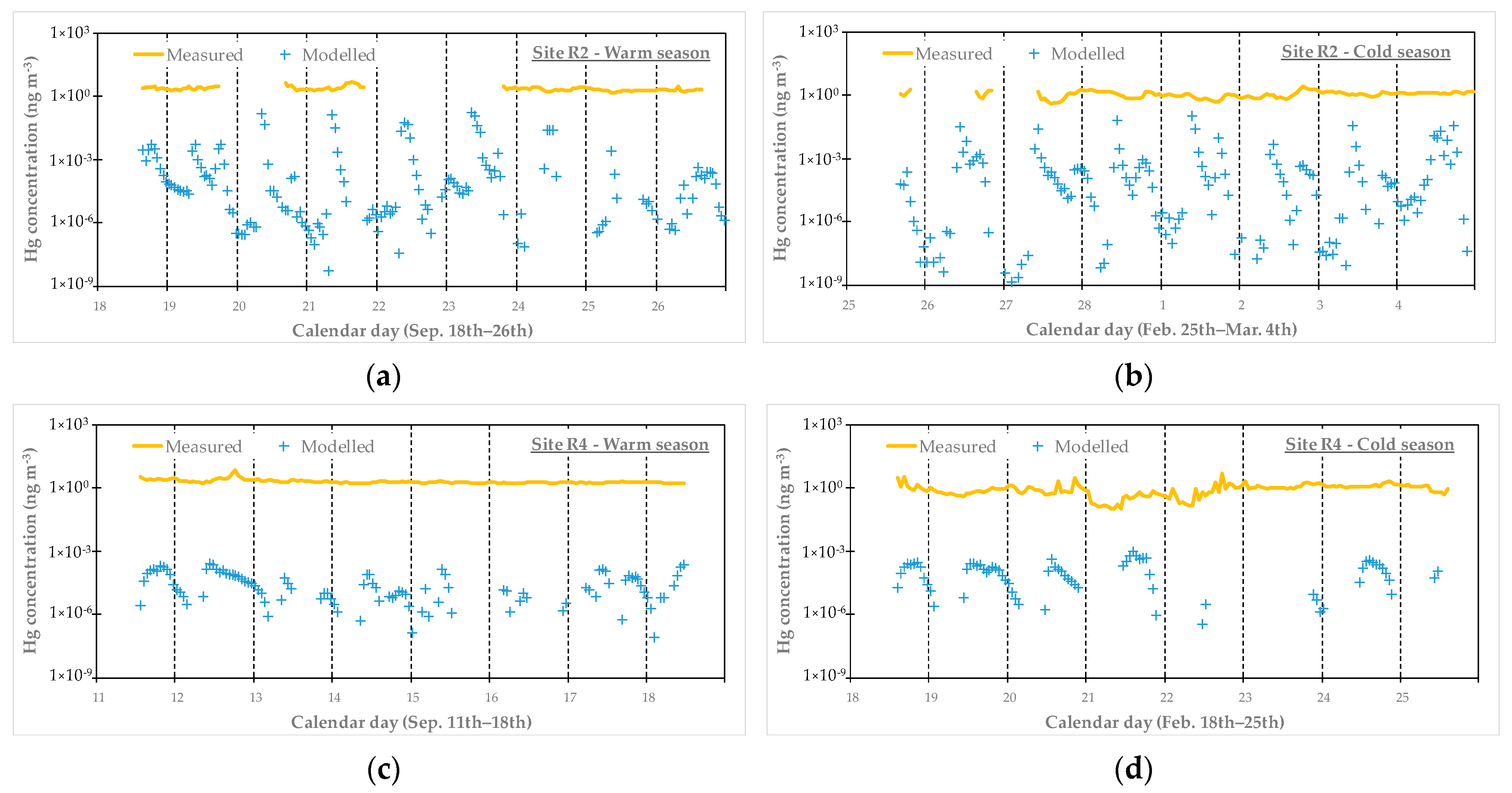
3.2.3. TGM
4. Conclusions
Supplementary Materials
Author Contributions
Funding
Institutional Review Board Statement
Informed Consent Statement
Data Availability Statement
Acknowledgments
Conflicts of Interest
References
- Egüez, A. Compliance with the EU waste hierarchy: A matter of stringency, enforcement, and time. J. Environ. Manag. 2021, 280, 111672. [Google Scholar] [CrossRef] [PubMed]
- European Commission. The Role of Waste-to-Energy in the Circular Economy. Communication from the Commission to the European Parliament, the Council, the European Economic and Social Committee and the Committee of the Regions, COM/2017/0034. Brussels, 26 January 2017. Available online: https://eur-lex.europa.eu/legal-content/EN/TXT/PDF/?uri=CELEX:52017DC0034 (accessed on 10 September 2021).
- Malinauskaite, J.; Jouhara, H.; Czajczyńska, D.; Stanchev, P.; Katsou, E.; Rostkowski, P.; Thorne, R.; Colón, J.; Ponsá, S.; Al-Mansour, F.; et al. Municipal solid waste management and waste-to-energy in the context of a circular economy and energy recycling in Europe. Energy 2017, 141, 2013–2044. [Google Scholar] [CrossRef]
- Liu, Y.; Ge, Y.; Xia, B.; Cui, C.; Jiang, X.; Skitmore, M. Enhancing public acceptance towards waste-to-energy incineration projects: Lessons learned from a case study in China. Sustain. Cities Soc. 2019, 48, 101582. [Google Scholar] [CrossRef]
- Song, J.; Sun, Y.; Jin, L. PESTEL analysis of the development of the waste-to-energy incineration industry in China. Renew. Sustain. Energy Rev. 2017, 80, 276–289. [Google Scholar] [CrossRef]
- Baxter, J.; Ho, Y.; Rollins, Y.; Maclaren, V. Attitudes toward waste to energy facilities and impacts on diversion in Ontario, Canada. Waste Manag. 2016, 50, 75–85. [Google Scholar] [CrossRef] [PubMed]
- Ren, X.; Che, Y.; Yang, K.; Tao, Y. Risk perception and public acceptance toward a highly protested Waste-to-Energy facility. Waste Manag. 2015, 48, 528–539. [Google Scholar] [CrossRef]
- European Union. Directive 2010/75/EU of the European Parliament and of the Council on Industrial Emissions (Inte-Grated Pollution Prevention and Control). Official Journal of the European Union L 334, 17 December 2010, 17–119. Available online: https://eur-lex.europa.eu/legal-content/EN/TXT/?uri=celex%3A32010L0075 (accessed on 10 September 2021).
- European Union. Commission Implementing Decision (EU) 2019/2010 of 12 November 2019 Establishing the Best Available Techniques (BAT) Conclusions, under Directive 2010/75/EU of the European Parliament and of the Council, for Waste incineration. Official Journal of the European Union L 312/55, 3.12.2019. Available online: https://eur-lex.europa.eu/legal-content/EN/TXT/PDF/?uri=CELEX:32019D2010&from=EN (accessed on 10 September 2021).
- Passarini, F.; Nicoletti, M.; Ciacci, L.; Vassura, I.; Morselli, L. Environmental impact assessment of a WtE plant after structural upgrade measures. Waste Manag. 2014, 34, 753–762. [Google Scholar] [CrossRef] [Green Version]
- Giusti, L. A review of waste management practices and their impact on human health. Waste Manag. 2009, 29, 2227–2239. [Google Scholar] [CrossRef]
- Hu, S.-W.; Shy, C.M. Health Effects of Waste Incineration: A Review of Epidemiologic Studies. J. Air Waste Manag. Assoc. 2001, 51, 1100–1109. [Google Scholar] [CrossRef]
- Cordioli, M.; Ranzi, A.; De Leo, G.A.; Lauriola, P. A Review of Exposure Assessment Methods in Epidemiological Studies on Incinerators. J. Environ. Public Heal 2013, 2013, 129470. [Google Scholar] [CrossRef] [Green Version]
- Cole-Hunter, T.; Johnston, F.H.; Marks, G.B.; Morawska, L.; Morgan, G.G.; Overs, M.; Porta-Cubas, A.; Cowie, C.T. The health impacts of waste-to-energy emissions: A systematic review of the literature. Environ. Res. Lett. 2020, 15, 123006. [Google Scholar] [CrossRef]
- Tait, P.W.; Brew, J.; Che, A.; Costanzo, A.; Danyluk, A.; Davis, M.; Khalaf, A.; McMahon, K.; Watson, A.; Rowcliff, K.; et al. The health impacts of waste incineration: A systematic review. Aust. N. Z. J. Public Health 2020, 44, 40–48. [Google Scholar] [CrossRef] [PubMed]
- de Titto, E.; Savino, A. Environmental and health risks related to waste incineration. Waste Manag. Res. J. Sustain. Circ. Econ. 2019, 37, 976–986. [Google Scholar] [CrossRef] [PubMed]
- Hoek, G.; Ranzi, A.; Alimehmeti, I.; Ardeleanu, E.R.; Arrebola, J.P.; ávila, P.; Candeias, C.; Colles, A.; Crian, G.C.; Dack, S.; et al. A review of exposure assessment methods for epidemiological studies of health effects related to industrially contaminated sites. Epidemiol. Prev. 2018, 42, 21–36. [Google Scholar] [CrossRef]
- Ashworth, D.C.; Elliott, P.; Toledano, M.B. Waste incineration and adverse birth and neonatal outcomes: A systematic review. Environ. Int. 2014, 69, 120–132. [Google Scholar] [CrossRef]
- Lonati, G.; Cambiaghi, A.; Cernuschi, S. The Actual Impact of Waste-to-Energy Plant Emissions on Air Quality: A Case Study from Northern Italy. Detritus 2019, 6, 77–84. [Google Scholar] [CrossRef]
- Scire, J.S.; Robe, F.R.; Fernau, M.E.; Yamartino, R. A User’s Guide for the CALMET Meteorological Model. 2000. Available online: http://src.com/calpuff/download/CALMET_UsersGuide.pdf (accessed on 5 September 2021).
- Scire, J.S.; Strimaitis, D.G.; Yamartino, R. A User’s Guide for the CALPUFF Dispersion Model. 2000. Available online: http://www.src.com/CALPUFF/download/CALPUFF_UsersGuide.pdf (accessed on 5 September 2021).
- Caserini, S.; Giani, P.; Cacciamani, C.; Ozgen, S.; Lonati, G. Influence of climate change on the frequency of daytime temperature inversions and stagnation events in the Po Valley: Historical trend and future projections. Atmos. Res. 2016, 184, 15–23. [Google Scholar] [CrossRef] [Green Version]
- Ferrario, M.E.; Rossa, A.M.; Pernigotti, D. Characterization of PM10 accumulation periods in the Po valley by means of boundary layer profiler. In Proceedings of the 14th ISARS–International Symposium for the Advancement of Boundary Layer Remote Sensing, Roskilde, Denmark, 13–15 June 2010. [Google Scholar]
- DIN EN 14181. Stationary Source Emissions–Quality Assurance of Automated Measuring Systems. Released 2015-02. Available online: https://www.en-standard.eu/din-en-14181-stationary-source-emissions-quality-assurance-of-automated-measuring-systems/ (accessed on 23 January 2022).
- ARPAV. Studio e Determinazione Delle Ricadute Dell’impianto di Termovalorizzazione di Schio. (In Italian). 2018. Available online: https://www.arpa.veneto.it/arpav/chi-e-arpav/file-e-allegati/dap-vicenza/aria/2018_0100988%20ALLEGATO%20Relazione.pdf/view (accessed on 20 September 2021).
- LAI (Länderausschuss für Immissionsschutz). Bericht des Länderausschusses für Immissionsschutz (LAI) Bewertung von Schadstoffen, für Die Keine Immissionswerte Festgelegt Sind Orientierungswerte für Die Sonderfallprüfung und für Die Anlagenüberwachung Sowie Zielwerte für Die Langfristige Luftreinhalteplanung unter Besonderer Berücksichtigung der Beurteilung krebsezrzeugender Luftschadstoffe. 2004. Available online: https://www.lanuv.nrw.de/fileadmin/lanuv/gesundheit/pdf/LAI2004.pdf (accessed on 20 September 2021).
- European Commission. Directive 2008/50/EC Directive 2008/50/EC of the European Parliament and of the Council of 21 May 2008 on Ambient Air Quality and Cleaner Air for Europe OJ L 152, 6 November 2008. pp. 1–44. Available online: http://eur-lex.europa.eu/legal-content/en/ALL/?uri=CELEX:32008L0050 (accessed on 10 September 2021).
- Conca, E.; Malandrino, M.; Giacomino, A.; Inaudi, P.; Buoso, S.; Bande, S.; Sacco, M.; Abollino, O. Contribution of the Incinerator to the Inorganic Composition of the PM10 Collected in Turin. Atmosphere 2020, 11, 400. [Google Scholar] [CrossRef] [Green Version]
- Khan, B.; Masiol, M.; Bruno, C.; Pasqualetto, A.; Formenton, G.M.; Agostinelli, C.; Pavoni, B. Potential sources and meteorological factors affecting PM2.5-bound polycyclic aromatic hydrocarbon levels in six main cities of northeastern Italy: An assessment of the related carcinogenic and mutagenic risks. Environ. Sci. Pollut. Res. 2018, 25, 31987–32000. [Google Scholar] [CrossRef]
- Silibello, C.; Calori, G.; Costa, M.P.; Dirodi, M.G.; Mircea, M.; Radice, P.; Vitali, L.; Zanini, G. Benzo[a]pyrene modelling over Italy: Comparison with experimental data and source apportionment. Atmos. Pollut. Res. 2012, 3, 399–407. [Google Scholar] [CrossRef] [Green Version]
- Patti, S.; Pillon, S.; Intini, B.; Susanetti, L. Action D3. Consumo Residenziale di Biomasse Legnose Nel Bacino Padano–Report Sull’indagine Per Stimare i Consumi di Biomasse Legnose Nel Residenziale. PREPAIR Project under EU LIFE 2014-2020 Programme (LIFE 15 IPE IT 013). 2020. Available online: http://www.lifeprepair.eu/wp-content/uploads/2017/06/D3_Report-indagine-sul-consumo-domestico-di-biomasse-legnose-1.pdf (accessed on 10 January 2022).
- ARPA VENETO. INEMAR Veneto 2017–Inventario Regionale Delle Emissioni in Atmosfera in Regione Veneto, Edizione 2017. ARPA Veneto–Dipartimento Regionale Qualità dell’Ambiente–Unità Organizzativa Qualità dell’Aria, Regione del Veneto–Area Tutela e Sicurezza del Territorio, Direzione Ambiente–UO Tutela dell’Atmosfera. Available online: https://www.arpa.veneto.it/dati-ambientali/open-data/file-e-allegati/emissioni-2017/INEMARVeneto2017_EmissCom_provVI.csv (accessed on 15 September 2021).
- Paglione, M.; Gilardoni, S.; Rinaldi, M.; Decesari, S.; Zanca, N.; Sandrini, S.; Giulianelli, L.; Bacco, D.; Ferrari, S.; Poluzzi, V.; et al. The impact of biomass burning and aqueous-phase processing on air quality: A multi-year source apportionment study in the Po Valley, Italy. Atmos. Chem. Phys. 2020, 20, 1233–1254. [Google Scholar] [CrossRef] [Green Version]
- NATO/CCMS. International Toxicity Equivalency Factor (I-TEF) Method of Risk Assessment for Complex Mixtures of Dioxins and Related Compounds. Pilot Study on International Information Exchange on Dioxins and Related Compounds, Report Number 176, August 1988, North Atlantic Treaty Organization, Committee on Challenges of Modern Society. 1988. Available online: https://nepis.epa.gov/ (accessed on 10 September 2021).
- Kutz, F.W.; Barnes, D.G.; Bretthauer, E.W.; Bottimore, D.P.; Greim, H. The international toxicity equivalency factor (I-TEF) method for estimating risks associated with exposures to complex mixtures of dioxins and related compounds. Toxicol. Environ. Chem. 1990, 26, 99–109. [Google Scholar] [CrossRef]
- Lonati, G.; Cernuschi, S.; Caserini, S. Organic and Inorganic Trace Pollutants around Municipal Solid Waste Incinerators: Results from Air Quality Monitoring Campaigns in Northern Italy. In Proceedings of the 1st International Conference on Applications of Air Quality in Science and Engineering Purposes, Kuwait City, Kuwait, 10–12 February 2020. [Google Scholar]
- Jiménez, J.C.; Eisenreich, S.; Mariani, G.; Skejo, H.; Umlauf, G. Monitoring atmospheric levels and deposition of dioxin-like pollutants in sub-alpine Northern Italy. Atmos. Environ. 2012, 56, 194–202. [Google Scholar] [CrossRef]
- Zain, S.M.S.M.; Latif, M.T.; Baharudin, N.H.; Anual, Z.F.; Hanif, N.M.; Khan, F. Atmospheric PCDDs/PCDFs levels and occurrences in Southeast Asia: A review. Sci. Total Environ. 2021, 783, 146929. [Google Scholar] [CrossRef]
- OSPAR Commission. OSPAR Background Document on Dioxins, Publication Number 308/2007, ISBN 978-1-905859-47-4. Available online: https://www.ospar.org/documents?v=7060 (accessed on 20 September 2021).
- Zhang, M.; Buekens, A.; Li, X. Dioxins from Biomass Combustion: An Overview. Waste Biomass Valorization 2017, 8, 1–20. [Google Scholar] [CrossRef]
- Piazzalunga, A.; Anzano, M.; Collina, E.; Lasagni, M.; Lollobrigida, F.; Pannocchia, A.; Fermo, P.; Pitea, D. Contribution of wood combustion to PAH and PCDD/F concentrations in two urban sites in Northern Italy. J. Aerosol Sci. 2013, 56, 30–40. [Google Scholar] [CrossRef] [Green Version]
- Dopico, M.; Gomez, A. Review of the current state and main sources of dioxins around the world. J. Air Waste Manag. Assoc. 2015, 65, 1033–1049. [Google Scholar] [CrossRef]
- Zhang, G.; Hai, J.; Cheng, J. Characterization and mass balance of dioxin from a large-scale municipal solid waste incinerator in China. Waste Manag. 2012, 32, 1156–1162. [Google Scholar] [CrossRef]
- Lin, W.-Y.; Wu, Y.-L.; Tu, L.-K.; Wang, L.-C.; Lu, X. The Emission and Distribution of PCDD/Fs in Municipal Solid Waste Incinerators and Coal-fired Power Plant. Aerosol Air Qual. Res. 2010, 10, 519–532. [Google Scholar] [CrossRef]
- Ni, Y.; Zhang, H.; Fan, S.; Zhang, X.; Zhang, Q.; Chen, J. Emissions of PCDD/Fs from municipal solid waste incinerators in China. Chemosphere 2009, 75, 1153–1158. [Google Scholar] [CrossRef]
- Passamani, G.; Rada, E.; Tirler, W.; Tava, M.; Torretta, V.; Ragazzi, M.; Brebbia, C.A.; Polonara, F.; Magaril, E.R.; Passerini, G. Pcdd/f emissions from virgin and treated wood combustion. Int. J. Energy Prod. Manag. 2017, 2, 17–27. [Google Scholar] [CrossRef] [Green Version]
- Lee, R.G.M.; Coleman, P.; Jones, J.L.; Jones, K.C.; Lohmann, R. Emission Factors and Importance of PCDD/Fs, PCBs, PCNs, PAHs and PM10 from the Domestic Burning of Coal and Wood in the U.K. Environ. Sci. Technol. 2005, 39, 1436–1447. [Google Scholar] [CrossRef] [PubMed]
- Lavric, E.D.; Konnov, A.A.; De Ruyck, J. Dioxin levels in wood combustion—A review. Biomass Bioenergy 2004, 26, 115–145. [Google Scholar] [CrossRef]
- Kentisbeer, J.; Leaver, D.; Cape, J.N. An analysis of total gaseous mercury (TGM) concentrations across the UK from a rural sampling network. J. Environ. Monit. 2011, 13, 1653–1661. [Google Scholar] [CrossRef] [Green Version]
- Sprovieri, F.; Pirrone, N.; Ebinghaus, R.; Kock, H.; Dommergue, A. A review of worldwide atmospheric mercury measurements. Atmos. Chem. Phys. 2010, 10, 8245–8265. [Google Scholar] [CrossRef] [Green Version]
- Kim, K.-H.; Yoon, H.-O.; Jung, M.-C.; Oh, J.-M.; Brown, R.J.C. A Simple Approach for Measuring Emission Patterns of Vapor Phase Mercury under Temperature-Controlled Conditions from Soil. Sci. World J. 2012, 2012, 940413. [Google Scholar] [CrossRef] [Green Version]
- Mason, R.P. Mercury Emissions from Natural Sources and their Importance in the Global Mercury Cycle. In Mercury Fate and Transport in the Global Atmosphere: Emissions, Measurements and Models; Mason, R.P., Pirrone, N., Eds.; Springer: Boston, MA, USA, 2009; pp. 173–191. [Google Scholar]
- Segal, M.; Mahrer, Y.; Pielke, R.A. A numerical model study of plume fumigation during nocturnal inversion break-up. Atmos. Environ. 1982, 16, 513–519. [Google Scholar] [CrossRef]
- Wang, I. On dispersion modeling of inversion breakup fumigation of power plant plumes. Atmos. Environ. 1977, 11, 573–576. [Google Scholar] [CrossRef]


| Parameter | Stack Line 1 and 2 | Stack Line 3 |
|---|---|---|
| Stack location x, y coordinate (km) | 687.152, 5064.883 | 687.165, 5064.868 |
| Stack height (m) | 40 | 40 |
| Stack diameter (m) | 1.6 | 1.3 |
| Actual flow rate (m3 h−1) | 89,730 [39,560–105,450] | 78,560 [48,415–99,930] |
| Temperature (°C) | 163.2 [136.1–176.2] | 141.1 [99.4–187.9] |
| Stack outlet speed (m s−1) | 12.4 [5.5–14.6] | 16.4 [4.15–20.9] |
| Parameter | Hg | Ni | Pb | BaP | PCDD/F |
|---|---|---|---|---|---|
| Geometric mean | 0.09 | 0.58 | 0.73 | 1.93 | 0.0027 |
| Geom. St. Dev. | 10.8 | 3.16 | 3.35 | 1.52 | 2.69 |
| Arithmetic mean | 0.28 | 1.12 | 1.52 | 2.38 | 0.0044 |
| Site | ARPAV Campaign | AVA Campaign (Warm Season) | AVA Campaign (Cold Season) |
|---|---|---|---|
| R2 | 4 June 2018–11 June 2018 | 11 September 2018–18 September 2018 18 September 2018–26 September 2018 | 18 February 2019–25 February 2019 25 February 2019–4 March 2019 |
| R3 | - | 18 September 2018–26 September 2018 | 25 February 2019–4 March 2019 |
| R4 | - | 11 September 2018–18 September 2018 | 18 February 2019–25 February 2019 |
| Pollutant | Air Quality Limit | Maximum Estimated |
|---|---|---|
| NO2 (µg m−3) | 40 | 2.7 |
| PM10 (µg m−3) | 40 | 2.0 × 10⁻² |
| BaP (ng m−3) | 1 | 5.8 × 10⁻⁵ |
| As (ng m−3) | 6 | 9.2 × 10⁻³ |
| Cd (ng m−3) | 5 | 9.2 × 10⁻³ |
| Ni (ng m−3) | 20 | 3.7 × 10⁻² |
| Pb (µg m−3) | 0.5 | 3.3 × 10⁻⁵ |
| Parameter | As | Cd | Ni | Pb | BaP |
|---|---|---|---|---|---|
| Meas. CS | <0.25 [<0.25] | 0.14 [0.05–0.6] | 2.2 [1.1–4.2] | 5.1 [1.4–13.6] | 0.31 [0.08–0.74] |
| Mod. CS | 5.2 × 10⁻⁴ [2.4 × 10⁻⁵–1.6 × 10⁻³] | 5.2 × 10⁻⁴ [2.4 × 10⁻⁵–1.6 × 10⁻³] | 9.6 × 10⁻⁴ [4.4 × 10⁻⁵–2.9 × 10⁻³] | 1.3 × 10⁻³ [6.0 × 10⁻⁵–4.0 × 10⁻³] | 2.3 × 10⁻⁶ [1.8 × 10⁻⁷–5.1 × 10⁻⁶] |
| Meas. WS | <0.25 [<0.25] | 0.07 [0.05–0.3] | 1.4 [0.5–2.8] | 2.9 [1.4–6.8] | 0.02 [0.005–0.08] |
| Mod. WS | 4.0 × 10⁻⁴ [1.8 × 10⁻⁵–9.4 × 10⁻⁴] | 4.0 × 10⁻⁴ [1.8 × 10⁻⁵–9.4 × 10⁻⁴] | 7.4 × 10⁻⁴ [3.4 × 10⁻⁵–1.8 × 10⁻³] | 1.0 × 10⁻³ [4.5 × 10⁻⁵–2.4 × 10⁻³] | 2.0 × 10⁻⁶ [3.3 × 10⁻⁷–7.0 × 10⁻⁶] |
| Relative contributions | |||||
| Mean CS | 0.21% | 0.66% | 0.05% | 0.03% | 0.001% |
| Max CS | 0.63% | 2.58% | 0.14% | 0.1% | 0.003% |
| Mean WS | 0.16% | 0.76% | 0.07% | 0.04% | 0.02% |
| Max WS | 0.38% | 1.89% | 0.33% | 0.16% | 0.12% |
| Site | Campaign | As | Cd | Ni | Pb | BaP | Hg | PCDD/F | |||||||
|---|---|---|---|---|---|---|---|---|---|---|---|---|---|---|---|
| Meas. | Mod. | Meas. | Mod. | Meas. | Mod. | Meas. | Mod. | Meas. | Mod. | Meas. | Mod. | Meas. | Mod. | ||
| R2 | 4 June–11 June 2018 | <1 | 7.0 × 10⁻³ | <0.2 | 7.0 × 10⁻³ | 1.80 | 1.3 × 10⁻² | 2.10 | 1.8 × 10⁻² | <0.02 | 2.8 × 10⁻⁵ | - | - | 0.2 | 5.0 × 10⁻² |
| 11 September–18 September 2018 | 0.32 | 1.3 × 10⁻² | 0.06 | 1.3 × 10⁻² | 1.16 | 2.5 × 10⁻² | 2.20 | 3.4 × 10⁻² | 0.006 | 5.3 × 10⁻⁵ | - | - | 6.1 | 9.5 × 10⁻² | |
| 18 September–26 September 2018 | 0.24 | 1.2 × 10⁻² | 0.08 | 1.2 × 10⁻² | 1.52 | 2.2 × 10⁻² | 1.84 | 3.0 × 10⁻² | 0.007 | 4.8 × 10⁻⁵ | 2.3 | 5.6 × 10⁻³ | 3.3 | 8.6 × 10⁻² | |
| 18 February–25 February 2019 | 0.43 | 5.5 × 10⁻³ | 0.17 | 5.5 × 10⁻³ | 2.21 | 1.0 × 10⁻² | 5.73 | 1.4 × 10⁻² | 0.53 | 2.2 × 10⁻⁵ | - | - | 14.1 | 3.9 × 10⁻² | |
| 25 February–4 March 2019 | 0.64 | 4.6 × 10⁻³ | 0.25 | 4.6 × 10⁻³ | 4.58 | 8.6 × 10⁻³ | 7.34 | 1.2 × 10⁻² | 0.51 | 1.8 × 10⁻⁵ | 1.1 | 2.2 × 10⁻³ | 15.2 | 3.3 × 10⁻² | |
| R3 | 18 September–26 September 2018 | 0.15 | 0.9 × 10⁻³ | 0.05 | 0.9 × 10⁻³ | 2.40 | 1.8 × 10⁻³ | 1.19 | 2.4 × 10⁻³ | 0.010 | 3.8 × 10⁻⁶ | - | - | 3.6 | 6.8 × 10⁻³ |
| 25 February–4 March 2019 | 0.61 | 1.7 × 10⁻³ | 0.18 | 1.7 × 10⁻³ | 6.25 | 3.2 × 10⁻³ | 5.79 | 4.3 × 10⁻³ | 0.40 | 6.8 × 10⁻⁶ | - | - | 11.3 | 1.2 × 10⁻² | |
| R4 | 11 September–18 September 2018 | 0.93 | 0.8 × 10⁻⁴ | 0.11 | 0.8 × 10⁻⁴ | 3.23 | 1.6 × 10⁻⁴ | 4.36 | 2.1 × 10⁻⁴ | 0.004 | 3.3 × 10⁻⁷ | 2.0 | 3.9 × 10⁻⁵ | 2.4 | 6.0 × 10⁻⁴ |
| 18 February–25 February 2019 | 0.64 | 1.5 × 10⁻⁴ | 0.13 | 1.5 × 10⁻⁴ | 2.60 | 2.8 × 10⁻⁴ | 4.71 | 3.8 × 10⁻⁴ | 0.64 | 6.0 × 10⁻⁷ | 0.9 | 7.0 × 10⁻⁵ | 17.3 | 1.1 × 10⁻³ | |
Publisher’s Note: MDPI stays neutral with regard to jurisdictional claims in published maps and institutional affiliations. |
© 2022 by the authors. Licensee MDPI, Basel, Switzerland. This article is an open access article distributed under the terms and conditions of the Creative Commons Attribution (CC BY) license (https://creativecommons.org/licenses/by/4.0/).
Share and Cite
Lonati, G.; Cernuschi, S.; Giani, P. Air Quality Impact Assessment of a Waste-to-Energy Plant: Modelling Results vs. Monitored Data. Atmosphere 2022, 13, 516. https://doi.org/10.3390/atmos13040516
Lonati G, Cernuschi S, Giani P. Air Quality Impact Assessment of a Waste-to-Energy Plant: Modelling Results vs. Monitored Data. Atmosphere. 2022; 13(4):516. https://doi.org/10.3390/atmos13040516
Chicago/Turabian StyleLonati, Giovanni, Stefano Cernuschi, and Paolo Giani. 2022. "Air Quality Impact Assessment of a Waste-to-Energy Plant: Modelling Results vs. Monitored Data" Atmosphere 13, no. 4: 516. https://doi.org/10.3390/atmos13040516