Article

Testing HYSPLIT Plume Dispersion Model Performance Using Regional Hydrocarbon Monitoring Data during a Gas Well Blowout

by
Gunnar W. Schade
* and
Mitchell L. Gregg
Department of Atmospheric Sciences, Texas A&M University, College Station, TX 77843, USA
*
Author to whom correspondence should be addressed.
Atmosphere 2022, 13(3), 486; https://doi.org/10.3390/atmos13030486
Submission received: 30 December 2021 / Revised: 12 March 2022 / Accepted: 14 March 2022 / Published: 17 March 2022
(This article belongs to the Special Issue Feature Papers in Atmosphere Science)

Abstract

:
A gas well blowout in south central Texas in November 2019 that lasted for 20 days provided a unique opportunity to test the Hybrid Single-Particle Lagrangian Integrated Trajectory (HYSPLIT) model’s plume dispersion against hydrocarbon air monitoring data at two nearby state monitoring stations. We estimated daily blowout hydrocarbon emission rates from satellite measurement-based results on methane emissions in conjunction with previously reported composition data of the local hydrocarbon resource. Using highly elevated hydrocarbon mixing ratios observed during several days at the two downwind monitoring stations, we calculated excess abundances above expected local background mixing ratios. Subsequent comparisons to HYSPLIT plume dispersion model outputs, generated using High-Resolution Rapid Refresh (HRRR) or North American Mesoscale (NAM) forecast meteorological input data, showed that the model generally reproduces both the timing and magnitude of the plume in various meteorological conditions. Absolute hydrocarbon mixing ratios could typically be reproduced within a factor of two. However, when lower emission rate estimates provided by the company in charge of the well were used, downwind hydrocarbon observations could not be reproduced. Overall, our results suggest that HYSPLIT, in combination with high-resolution meteorological input data, is a useful tool to accurately forecast chemical plume dispersion and potential human exposure in disaster situations.

1. Introduction

Human exposure to potentially harmful air pollutants is typically considered in two forms: chronic or acute exposure. Chronic exposure tends to be dominated by ubiquitous air pollutants emitted from many different sources, both natural and anthropogenic in nature; carbon monoxide and particulate matter (PM) are examples. In comparison, acute exposures are generally to much higher concentrations and tend to be short-term in nature. They are often caused by sometimes deliberate, but usually accidental releases of chemicals into the air from single, defined locations where the potentially hazardous materials are handled. If those chemicals are regulated, any emissions have to be reported to the regulatory agency unless the released amounts fall below de minimis thresholds. In the State of Texas, U.S.A., if exceeding said state-set threshold, regardless of whether the emissions were deliberate or accidental, the responsible party is required to terminate the emissions as soon as possible, and subsequently submit an emission event report to the Texas Commission on Environmental Quality (TCEQ).
Emission events (EEs) have significantly increased in Texas in recent years. Depending on the magnitude, duration, and types of air pollutant emissions from such events, local or regional air quality (AQ) monitoring may be performed by TCEQ during the event, and even site evacuations have been prompted to protect people from harm. An incident that exemplifies this scenario is a gas or oil well blowout in a populated area. Depending on weather conditions, and the duration of the blowout event, hydrocarbon emissions from the well may represent both an explosion hazard in the near-field of the blowout (within 1–2 km), as well as a significant health hazard, requiring incident response teams to make timely decisions about possible evacuations and necessary AQ monitoring as the event further develops. Mid- and far-field dispersion of the emitted pollutants tend to be of lesser concern unless the pollutants are of high toxicity or can have significant environmental impacts. Examples include radioactivity or fire smoke emissions, but also hydrocarbons due to individual toxicity (e.g., benzene) or their secondary ozone formation in the atmosphere.
The Hybrid Single-Particle Lagrangian Integrated Trajectory (HYSPLIT) model has been a widely used tool to determine air mass trajectories and pollutant dispersion for over twenty years [1,2,3,4,5,6,7,8,9,10,11,12,13]. The model, housed and maintained by the US National Oceanic and Atmospheric Administration (NOAA), is publicly available online (http://ready.arl.noaa.gov/HYSPLIT.php, accessed on 10 March 2022). It can be run online or offline using archived meteorological data of various spatial resolutions for regional or global air mass trajectory or pollutant dispersion analyses [9]. The National Weather Service (NWS), through its nationwide weather forecasting offices (WFOs), is already using HYSPLIT to analyze potential and actual hazardous materials releases into the atmosphere to provide guidance for decision makers on the ground, such as police departments, fire-fighters, or hazmat personnel. Its response time can be as short as 10 min after notification of an incident. A recent example is the Valero refinery fire, a typical incident classified as an EE, for which the WFO in Corpus Christi provided a HYSPLIT model run to the City of Corpus Christi Office of Emergency Management in April 2017.
The scientific user community of HYSPLIT has been improving the model at various stages in its history. The most recent updates, which were tested and implemented in 2020, include a new dispersion algorithm adopted from the Stochastic Time-Inverted Lagrangian Transport (STILT) model [14], as well as new turbulence and boundary layer depth parameterization schemes previously used in STILT. The additions were recently described in detail by Loughner et al. [15]. The updates created a significantly increased number of choices of algorithms and parameterizations in HYSPLIT Version 5, which the authors tested against archived tracer release experiment data, such as from CAPTEX [16]. Significant improvements of model performance were obtained for the subset of models that used the new STILT dispersion algorithm, which causes less vertical dispersion, an aspect previously found leading to underestimates of pollutant concentrations in the boundary layer [2], when HYSPLIT Version 4 was used.
The appropriate use of meteorological input data can be crucial to accurately forecast pollutant dispersions. Since 2019, routine High-Resolution Rapid Refresh (HRRR) data at 3 km spatial resolution for North America is available for use with HYSPLIT (https://rapidrefresh.noaa.gov/hrrr/, accessed on 14 March 2022). The previously highest-resolution met-data for the US was the North American Mesoscale (NAM) model (12 km). While scientific users may generate higher-resolution input data using the Weather Research and Forecasting (WRF) model, HRRR and NAM data are operationally available and can be downloaded within minutes to hours. In contrast, WRF model application can be time consuming and is thus not ideal for the rapid response often required with emission events, especially those of a hazardous nature.
In this project, we tested the performance of HYSPLIT Version 5.1 in dispersing a gas well blowout hydrocarbon plume in the Eagle Ford shale in south central Texas. We compared HRRR input data with regional met-station data, and HYSPLIT dispersion model outputs with hourly air quality monitoring data from two downwind locations.

2. Materials and Methods

2.1. Fidelity of HRRR Data

To ensure that the HRRR forecast data accurately represented the real-world weather in our region of interest, comparisons were made between direct observations from several weather stations and 00Z HRRR model initializations for the same time as the observations. Five locations surrounding the blowout site in Dewitt County were examined for four different weeks throughout the year. These four weeks allowed us to examine how the HRRR initialization performed during different seasons of the year, giving us a more complete picture of how the HRRR meteorological model compares to station measurements. The four weeks selected were 1–7 January, 1–7 April, 1–7 July and 1–7 October 2019 as they each represented a different season.
For each hour of each day in each of the four weeks of interest, 00Z HRRR data were downloaded as GRIB files, opened using the NOAA Weather and Climate Toolkit, and converted into a readable CSV format. During this GRIB-to-CSV conversion process, only variables of interest were selected: 2 m air temperature and 10 m winds (speed and direction). Data was bounded between 28 and 30 degrees latitude, and −96.6 and −98.6 degrees longitude. This resulted in a separate, unique CSV file for each variable at each hour for each day in our region. Spreadsheets were used to combine these files into a larger, weekly CSV file for each variable.
To determine the local fidelity of this HRRR data, local weather station data was retrieved from 5 locations in the region; Gonzales, Beeville, Fayette, New Braunfels, and Victoria. CSV files of hourly wind speed, wind direction, and temperature values were created for each location, for all of 2019. Each of these stations reports their respective values at slightly different times and/or intervals, so filtering was used to focus on only the values nearest to each whole hour, so as to line up with the hourly data from the HRRR model.
Lastly, the HRRR data was filtered by each station’s latitude and longitude combination, compiling each variable into a master spreadsheet for each weather station location. All master spreadsheets are made available through the Texas data repository.

2.2. HYSPLIT Processing

HYSPLIT Version 5.1 was installed on a local PCs in spring 2021. The newer HYSPLIT version includes advanced computational methods, including a new dispersion computation approach called the Stochastic Time-Inverted Lagrangian Transport (STILT) model, designed following the original work of Lin et al. [14]. According to the HYSPLIT manual, the STILT mixing scheme sets up several additional computations:
  • An internal forward-backward transport scheme to correct for violations of mass consistency in the meteorological fields,
  • The definition of additional layers near [the top of the boundary layer] to reduce particle trapping in that stable environment,
  • A probability scheme for particle reflection/transmission across interfaces with step changes in turbulence, and
  • A finer internal time step to reduce the errors introduced by operator splitting.
The incorporation of STILT into HYSPLIT was recently described by Loughner et al. (2021, [15]). Most importantly, they include (i) a more detailed algorithm for estimating boundary layer height, (ii) a new turbulence parameterization, (iii) a vertical Lagrangian timescale that varies in time and space, (iv) a complex dispersion algorithm, and (v) two new convection schemes. Testing by the authors and HYSPLIT developers showed that peak (downwind) concentrations were often in better agreement with measured peak values (likely due to less vertical dispersion), but overall the STILT scheme results were comparable to the original calculations using (default settings) HYSPLIT mixing schemes.
With these changes in setup in mind, we carried out a set of HYSPLIT runs using HRRR 3 km and NAM 12 km resolution meteorological input data, summarized in Table 1. We used a generic emission source at 28.9928 N, −97.6125 W, and 10.0 m agl. (unit: h−1), which leads to a calculation output at each grid cell of unit m−3, which, when multiplied with a known emission source strength in mass units, produces a concentration unit (e.g., g m−3) at the receptor grid cell locations.
Each model run included a spin-up period of 30 h, and a data period of 24 h. The last 24 h corresponded to one each of the first 20 days in November 2019 during which the emissions plume from the gas well blowout location was dispersed into the atmosphere. Output was set at average concentration for each hour, leading ultimately to 20 individual 24 h datasets of gridded (mass) dilution ratios across a 3 × 3 degree domain surrounding the blowout location.
These model outputs were converted to ASCII files and subsequently processed in R [17]. The gridded dilution ratio data were multiplied with calculated, average (as well as upper and lower) daily mass emissions rates for ethane (see below), and then converted to molar mixing ratios (ppb) in each grid cell. Ethane was chosen because it was the next most abundant hydrocarbon emitted after methane, is routinely measured using auto-GCs at TCEQ air quality monitoring stations, and is therefore likely detectable above background mixing ratios in the area for the largest distances encountered. In addition, auxiliary information was available for the likely ethane-to-methane ratios in the blowout from raw hydrocarbon composition measurements of the source rock provided in emission permit applications from the area accessed via TCEQ databases.

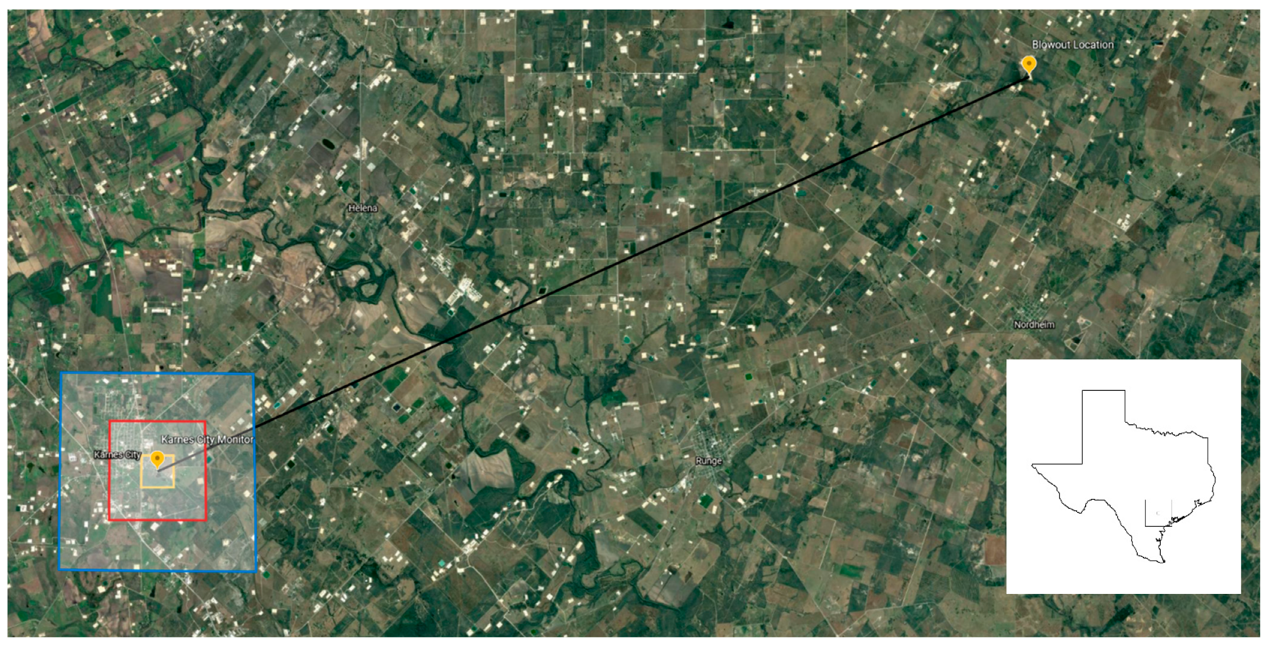
2.3. Study Site and Emission Rates

Figure 1 provides an overview of the study area in the Eagle Ford shale of south central Texas, highlighting both the blowout site and the main receptor studied in this project, the TCEQ air quality monitor in Karnes City, 29.6 km from the blowout location. The three boxes surrounding the receptor mark 1, 3, and 6 km size grid cells used for averaging model output.
Mass emission rates at the blowout site were expected to be provided by the responsible party in its emission event report to TCEQ. However, the report, as obtained in late fall of 2020, did not specify the hydrocarbons emitted but contained only a sum of “natural gas” emissions over the complete 20 day period the blowout lasted before the well was shut in. Furthermore, the reported amount was approximately 3-fold lower than what had been calculated from remotely sensed atmospheric methane via a multi-sensor, multi-satellite data analysis [18]. We therefore used the respective satellite measurements based emission rates over the period investigated, assuming an exponential drop of emissions over time, and developing a continuous time series using regression analysis as described below.

3. Results and Discussion

Our analysis is presented in three parts: In Section 3.1, we explain the calculation of ethane emission rates from the blowout site and discuss the excess hydrocarbon molar mixing ratio data at the two TCEQ air monitoring station receptor sites; in Section 3.2, we compare the HYSPLIT meteorological data with weather station data; in Section 3.3, we compare the observed hydrocarbon ratios near the blowout site with both the permit data and the observations at the AQ monitors; and in Section 3.4, we compare the modeled ethane data at the receptor sites with the excess ethane observations.

3.1. Blowout Emissions and Air Quality Monitor Measurements

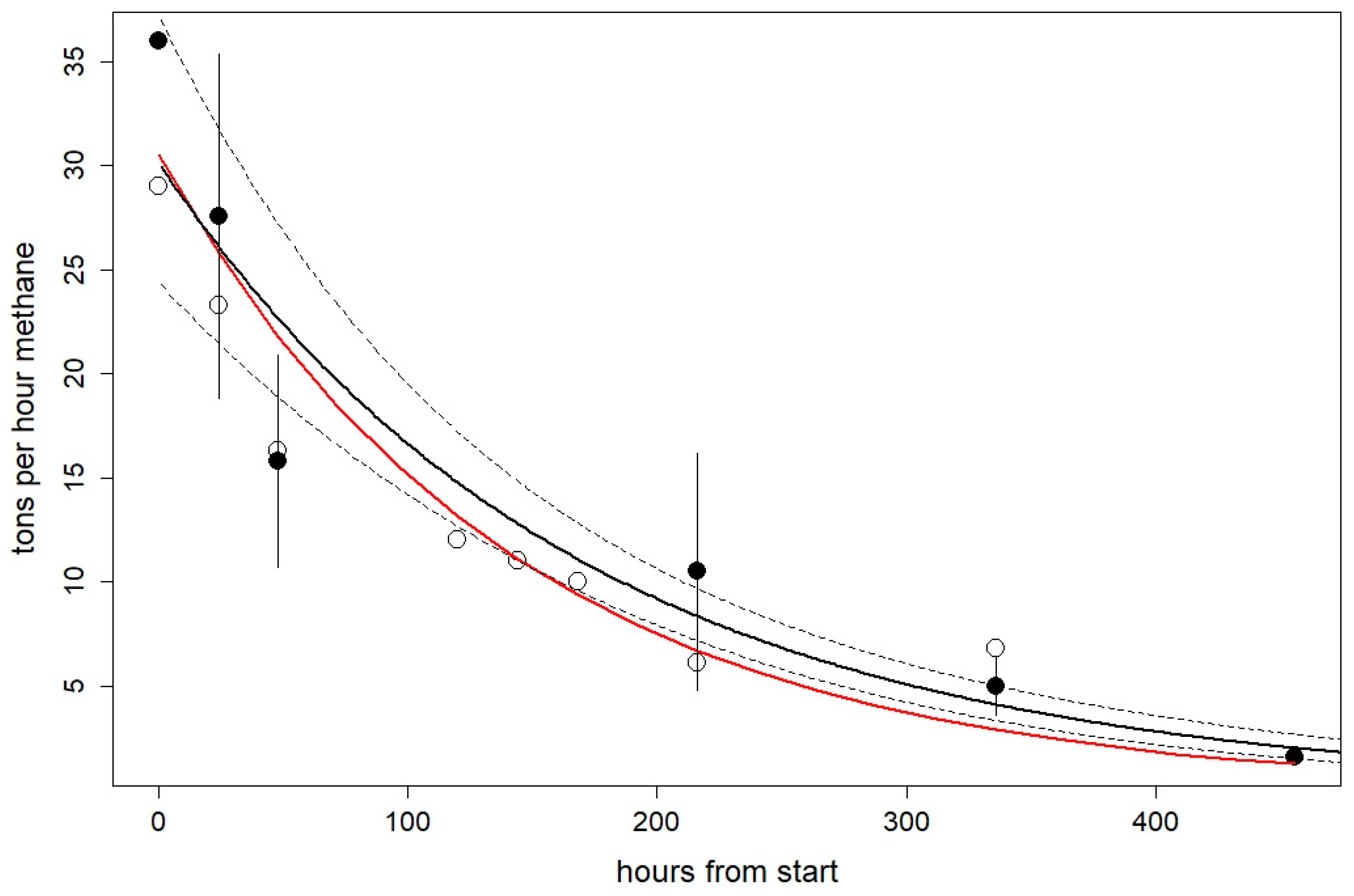
3.1.1. Emissions Calculations

The entity owning the gas well undergoing the blowout reported, and TCEQ accepted, a total emission amount of “natural gas” of 3.24 million pounds (TCEQ Investigation Report #1622284, October 2020; page 4). This translates into 1.47 million kg, or 1470 metric tons, most of which is (typically 80–95% of natural gas) in the form of methane. No explanation was given on how the operator arrived at that specific amount, and what composition the “natural gas” emitted had. An independent study using multiple sensors on various satellite platforms [18] evaluated the methane observations from this specific blowout and estimated that 4800 ± 980 metric tons of methane were likely emitted, more than 3-fold the amount estimated by the operator of the blowout well.
We used Figure 1 in Cusworth et al. [18], which shows a time series of methane emission estimates as observed from space, data given in the text, and data provided in Table S4 in the paper’s Supplementary Materials to create a new, continuous hourly emissions estimate, including uncertainty estimates. First, based upon the fact that a blowout is driven by well pressure, we assumed the change over time to follow an exponential decay curve. Second, unlike Cusworth and coworkers, we did not conservatively assume that day 1 (1 November 2019) emissions equaled day 2 observations, but chose two alternatives: (i) that the November 1 emission rate was the mean minus one sd of the November 2 combined TROPOMI satellite and WRF dispersion-based estimate (29 t/h), and (ii) that the November 1 emission rate was the mean plus one sd of the November 2 TROPOMI satellite Integrated Methane Enhancement (IME)-based estimate (36 t/h). These two values likely bracket the first day’s emission rate, which was undoubtedly higher than the estimate for November 2 (27.6 t/h).
Figure 2 shows all measured data points as filled circles, and all additional, OCI model (Table S4 in [18])-based estimates as open circles. Vertical error bars reflect the original 1-sd uncertainty estimates given by Cusworth et al. [18]. The Oil Climate Index (OCI) model-based data are included as open circles; they reflect methane emissions over the course of the blowout event estimated using inputs on reservoir composition and pressures as obtained from the Texas oil and gas regulatory body, the Texas Railroad Commission (Supplementary Materials Section S6 in Cusworth et al. [18]).
Next, we carried out a measurement data-weighted linear least-squares regression on log-transformed data, which provided a mean model (solid black line) and 95% confidence limit (solid dashed lines) output for all hours of the regression. A similarly weighted non-linear least squares regression is included in Figure 2 (red line) for comparison. This led to a slightly steeper initial drop in emission rates. The first method leads to a total emission amount of 4765 (+929, −774) tons for the 20 days of the event, the second to 4179 tons. Both new estimates are, as expected, well within the original estimate of 4800 ± 980 metric tons from Cusworth et al. [18], from which they were derived.
Next, an average daily (24 h) emission rate and its relative uncertainty were calculated from the hourly resolution curves in Figure 2. For the last step, to derive ethane emissions, information on the relative ethane-to-methane ratio in blowout emissions is necessary, but was unavailable. We thus relied on the information on source rock hydrocarbon composition gathered by Cusworth et al. [18] (cf. their Table S1), and from local emissions permit applications, including the actual application for the well in question, which used the same hydrocarbon composition evaluated at another well in the area in prior years (Section 3.3). While we will discuss hydrocarbon ratios derived from these permit applications vs. locally measured ratios further below, the relevant ethane-to-methane ratio adopted here is 15 ± 3% on a molar basis, and it was assumed to be invariant with time during the blowout. The estimated 20% relative uncertainty in this ratio was added to the methane emission relative uncertainty for all calculations. The final product was an emissions matrix with a daily mean, lower and upper ethane estimate for 1–20 November 2019, ranging from 11.3 t/h (November 1 maximum) to 0.2 t/h (November 20 minimum).

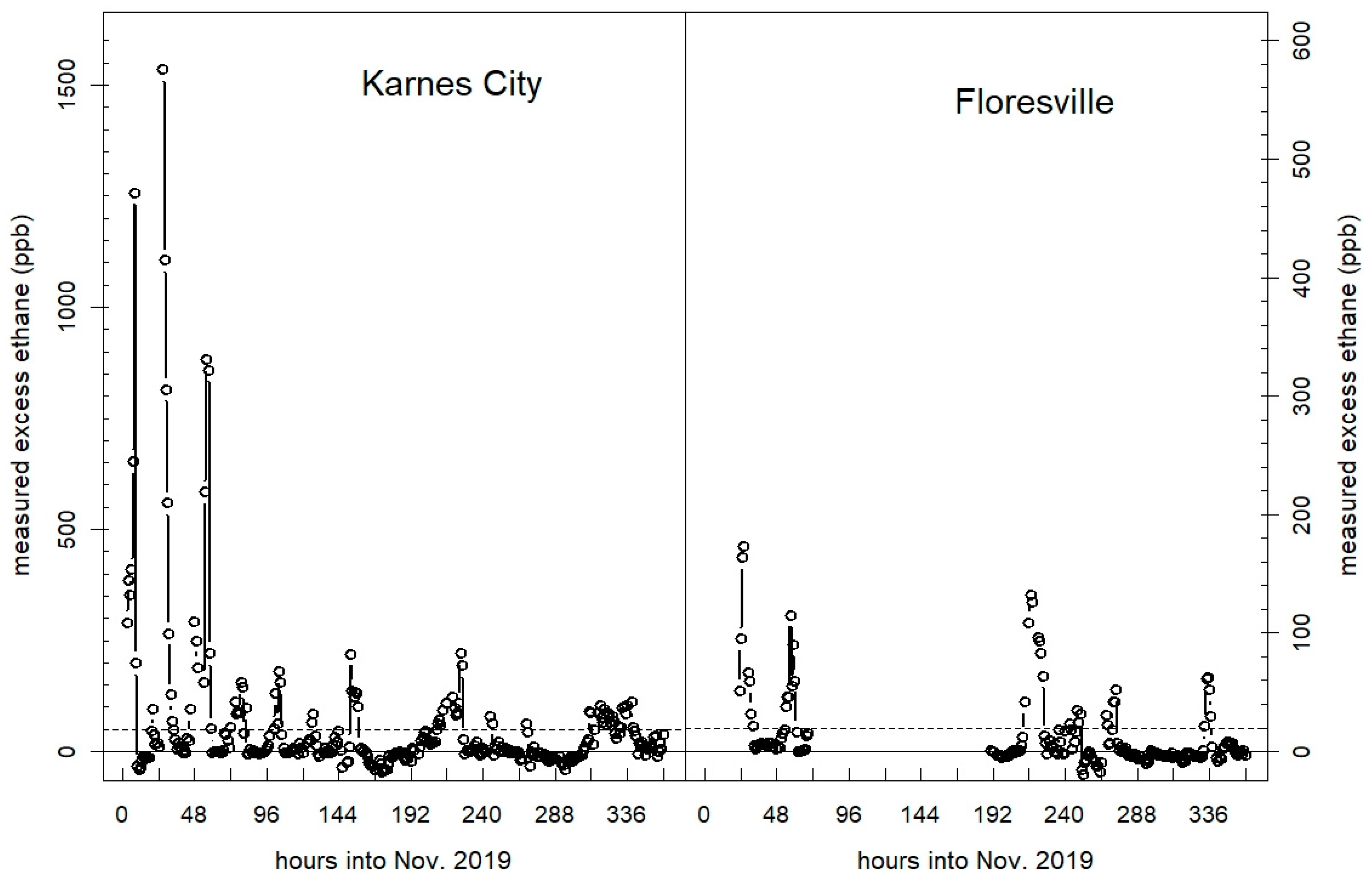
3.1.2. Excess Hydrocarbon Abundance at State Monitoring Sites

Monitoring data from the state’s Karnes City (AQS Site: 482551070, 1100B East Main Avenue, Karnes City, TX 78118, Lat: 28.88 N, Lon −97.89 W) and Floresville (AQS Site: 484931038, 1404 Hospital Blvd., Floresville, TX 78114, Lat: 29.13 N, Lon: −98.15 W) auto-GC instruments from 2019 were downloaded from TCEQ’s website and processed in fall 2020. The period in question, 1–20 November 2019, was separated from the rest of the data, and investigated for its meteorological conditions (Figure 3). We isolated four distinct periods, separated by vertical dashed green lines in Figure 3, with similar meteorological conditions, such as northerly winds with low temperatures behind frontal passages (from 7 to 10 November). For each period, a wind rose was constructed and a temperature range determined, to delineate the near consistent meteorological conditions.
The period delineations were used to sub-select a range of “reference” conditions from the remainder of the 2019 dataset, i.e., the complete set of 2019 data not including the blowout period. Meaning, representative median, interquartile, and 95% confidence level ranges of selected hydrocarbons at the monitor were calculated for each hour of the day for a given set of meteorological conditions derived from a meteorologically consistent period during the blowout event. These are considered representative reference conditions because they include all measurements that occurred before and after the blowout event but during otherwise similar meteorological conditions. This also implicitly includes a presumption of similar regional emissions conditions, aka that no substantial regional emissions developments (neither an increase nor decrease) occurred in 2019. This assumption was supported using oil and gas production data for Karnes and Dewitt counties, alongside a presumed proportionality between production and emission numbers, as is commonly done, e.g., by the EPA.
As an example, Figure 4 shows the determined reference levels of ethane in form of a diurnal boxplot overlaid with the actual ethane measurements at the Karnes City monitor for October 31, just before the blowout, and November 1–2, the first two days of the blowout. Again, ethane was selected due to its high emissions from the well, its continuous hourly local measurements, and its lack of other sources making it an excellent indicator species for oil and gas production related emissions. Note that ethane levels on the day before the blowout were lower than median reference levels until the late afternoon, when abundances started to exceed the 95% level of the reference periods. The highest ethane levels were reported for 2 November at 2–3 a.m. local time (LT), exceeding 1500 ppb, a day after the blowout was discovered. Outlier observations during the reference period (open circles in Figure 4) during these nighttime hours reached at most 50% of the ethane maxima, and median reference levels were typically an order of magnitude lower. Subsequent daytime levels on 1–2 November remained elevated above the reference.
This background reference calculation was performed for both receptor sites and for all five periods during which the blowout commenced, before the diverted gas was ignited on 14 November 2019. Enhancements (=excess ethane) over the reference data (medians of reference periods) were found for several days, significantly during the first week after the blowout occurred, shown in Figure 5 (unfortunately, four days of data from the Floresville site were either lost or did not pass TCEQ quality control checks). Due to sufficient vertical dispersion during daytime, typically only small enhancements were discovered for those hours, while all enhancements constituting order-of-magnitude effects occurred during nighttime, particularly after midnight, or around the dawn hours. Based upon the variability of the reference ethane levels through all five periods, we conservatively estimated that excess ethane below 50 ppb at Karnes City, and below 20 ppb at Floresville, could have been caused by sources other than the blowout. Notably, in the case of the Floresville site, ethane mixing ratios of a similar magnitude as shown in Figure 5 (100–200 ppb) were also encountered during the week just before the blowout period.

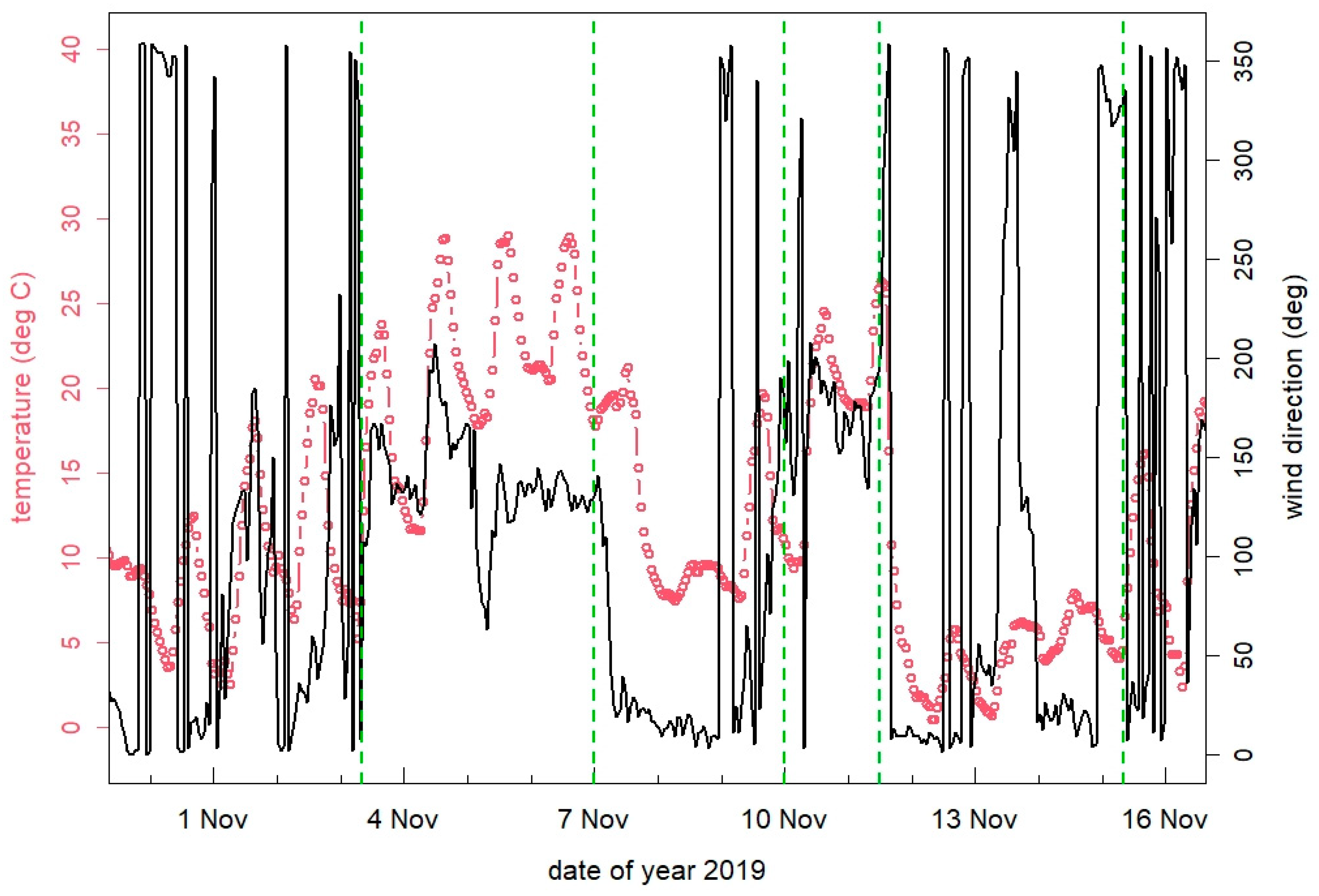
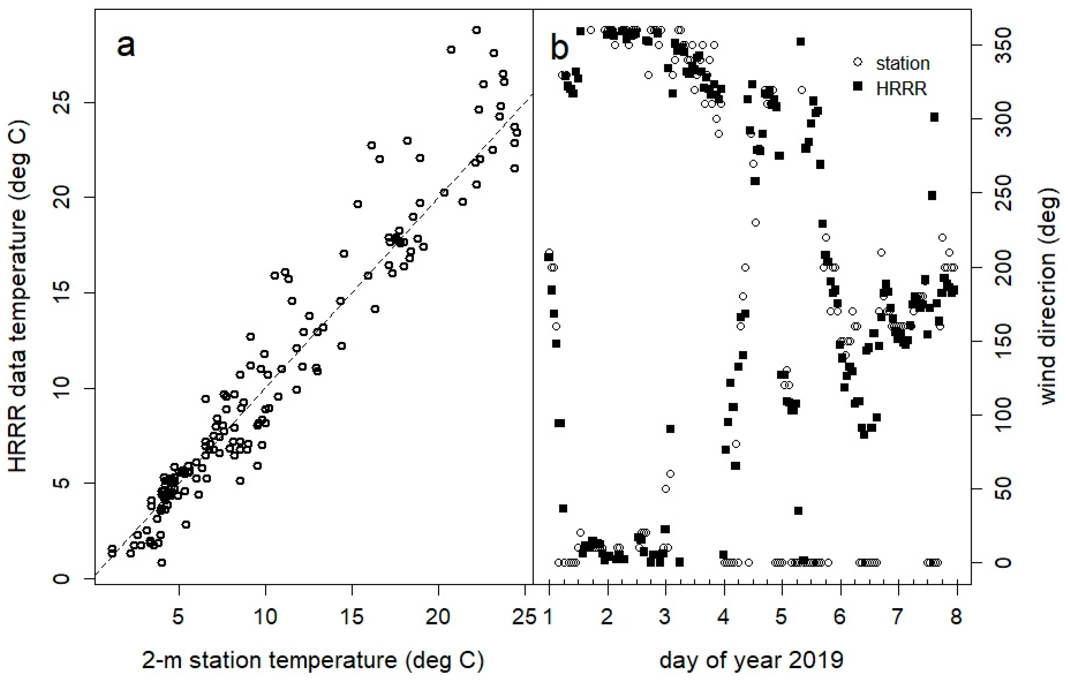
3.2. Comparisons of HYSPLIT Meteorological Input Data with Regional Measurements

Our comparisons between HRRR and local met-data showed an overall high fidelity of the HRRR data in this area of Texas. The master spreadsheets for all sites are provided as an extension to this manuscript in the Texas data repository. Here, we discuss two examples for one site, one for temperature and one for winds.
Figure 6a shows a scatter plot comparison of temperature data from a weather station near Gonzales, TX, approximately 60 km NNE of the blowout location, with HRRR data from the grid cell covering the station. In this example, the determination coefficient was 0.94 and the slope indicated a slightly higher HRRR estimate (5%) of the actual station temperature, on average. A similar result was obtained from other weather stations in the area during this winter period. The obtained mean error (ME) and mean bias (MB) were approximately 1.1 and 0.3 deg. C, respectively.
Figure 6b shows a time series comparison of wind direction data from the same station. Wind direction is a critical parameter for air mass transport, and, in this example, showed a very good comparison, capturing direction changes correctly when winds at the station were not calm (equates to a value of zero, in which case wind direction is not defined). Mean error and bias results (wind direction: MB = 3 deg., ME = 12 deg.; wind speed: r2 = 0.67, MB = −0.2 mph, ME = 1.8 mph; 1 mph = 0.45 m s−1) for this example were similar for winds at other sites. Meaning, nearly unbiased and closely correlated relationships were obtained. Similar to the temperature data, this indicates a high fidelity of the HRRR model winds for this area, and thus a high fidelity of the HYSPLIT meteorology inputs. Since we observed similar results at the other stations and for all seasons, we concluded that HRRR input data in general is likely of high to very high fidelity in this part of Texas, supporting its usage in the blowout event analysis.

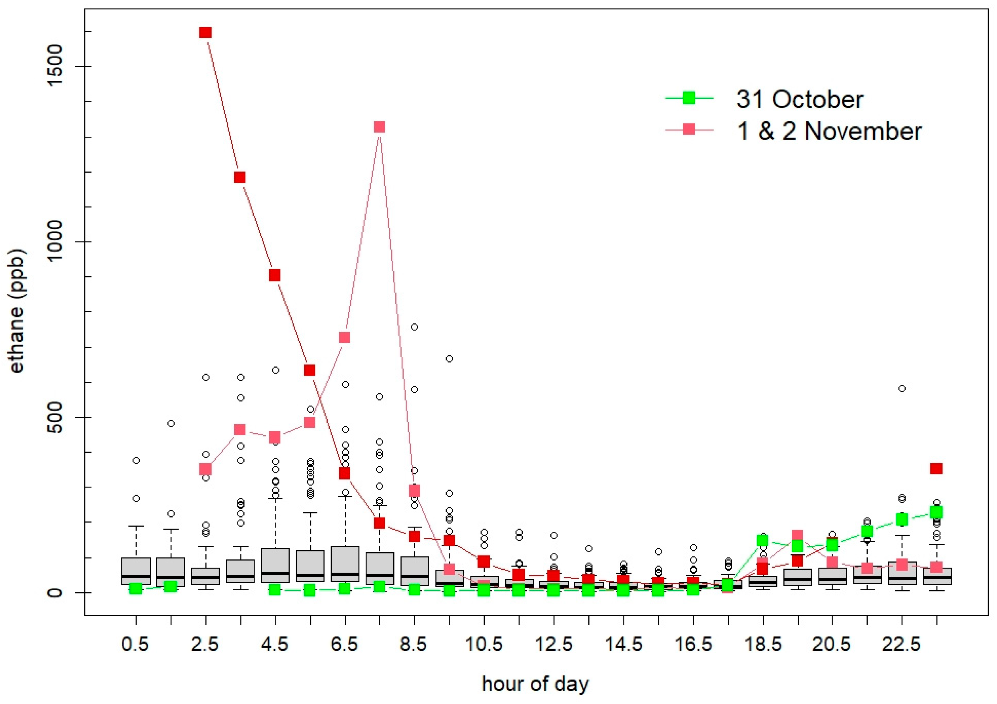
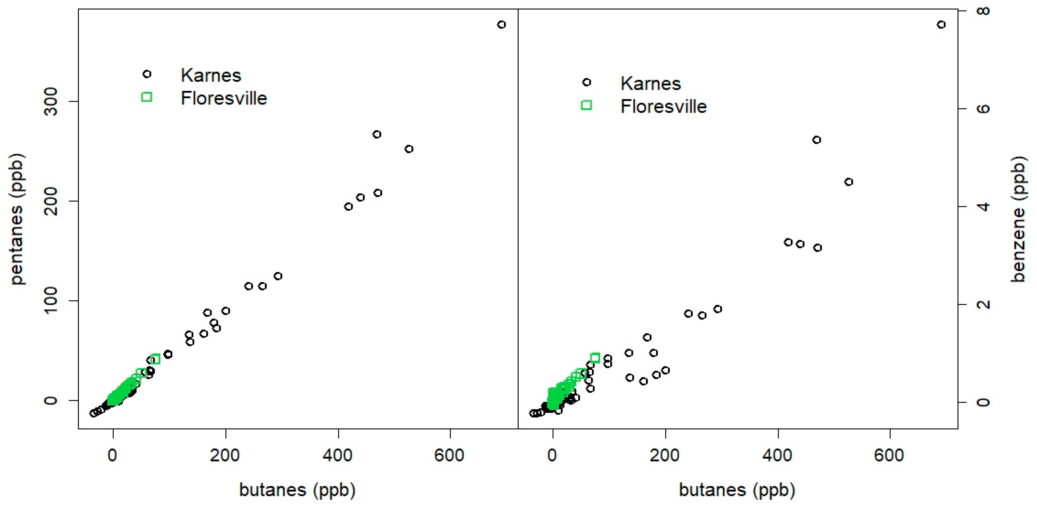
3.3. Hydrocarbon Composition

We used the excess levels above median reference levels to determine the hydrocarbon composition of blowout emissions as observed at the Karnes City and Floresville Hospital monitors. While neither the company’s report, nor the TCEQ investigation of the blowout listed its hydrocarbon composition, we obtained several measurements to compare the air monitor’s data to: (i) a 2009 local wildcat gas and well-stream composition analysis (well name: Migura 1) of the same field the blowout occurred in; (ii) a 2017 gas composition analysis from a standard permit application to TCEQ by Devon (Migura 3, pad 3), also of the same field the blowout occurred from; and (iii) a partial ambient gas composition analysis obtained from 24 h canister sampling carried out within a 2-mile radius near the blowout by a company contracted by the well’s owner, and provided in the Texas data repository.
Table 2 lists observed hydrocarbon ratios compared to the permit and near-field data. While the available ratios were generally comparable, in almost all cases the measured ratios at the downwind air quality monitor slightly deviated from the well gas composition in the direction of higher amounts of the less volatile hydrocarbon. This is to be expected because condensable hydrocarbons (“condensate”), such as BTEX and alkanes with five or more carbon atoms, are emitted with the gas during a blowout, but are not likely to be deposited to a large extent during plume dispersion. When surface deposition becomes a significant loss process of emitted condensate—typically at or near the blowout location during initial dispersion—we expect to find the observed composition downwind to deviate from the blowout well’s overall hydrocarbon composition (“well-stream”).
The excess hydrocarbon mixing ratios were highly consistent between the two monitoring sites, as is demonstrated for two examples in Figure 7. Differences in slope are likely insignificant. They could result from both slight calibration differences between the sites, and small statistical deviations due to the smaller amount and range of values available from the Floresville monitor. Differences to the local measurements near the ongoing blowout, and to the permit application data, probably also included effects from both (i) analytical methodology differences (much different for the onsite company measurements), and (ii) variability in the hydrocarbon source composition.
In summary, these comparisons suggest that excess hydrocarbon observations near the blowout were consistent with the expected hydrocarbon composition from the source, and were also consistent with distant downwind observations of excess hydrocarbons at two air quality monitors. Local condensate accumulation near the blowout was observed, and therefore some deposition had to have occurred. This, as well, is consistent with the observation that the B/T ratio (toluene being the lowest vapor pressure hydrocarbon investigated) was higher at the air quality monitors than what was observed locally.

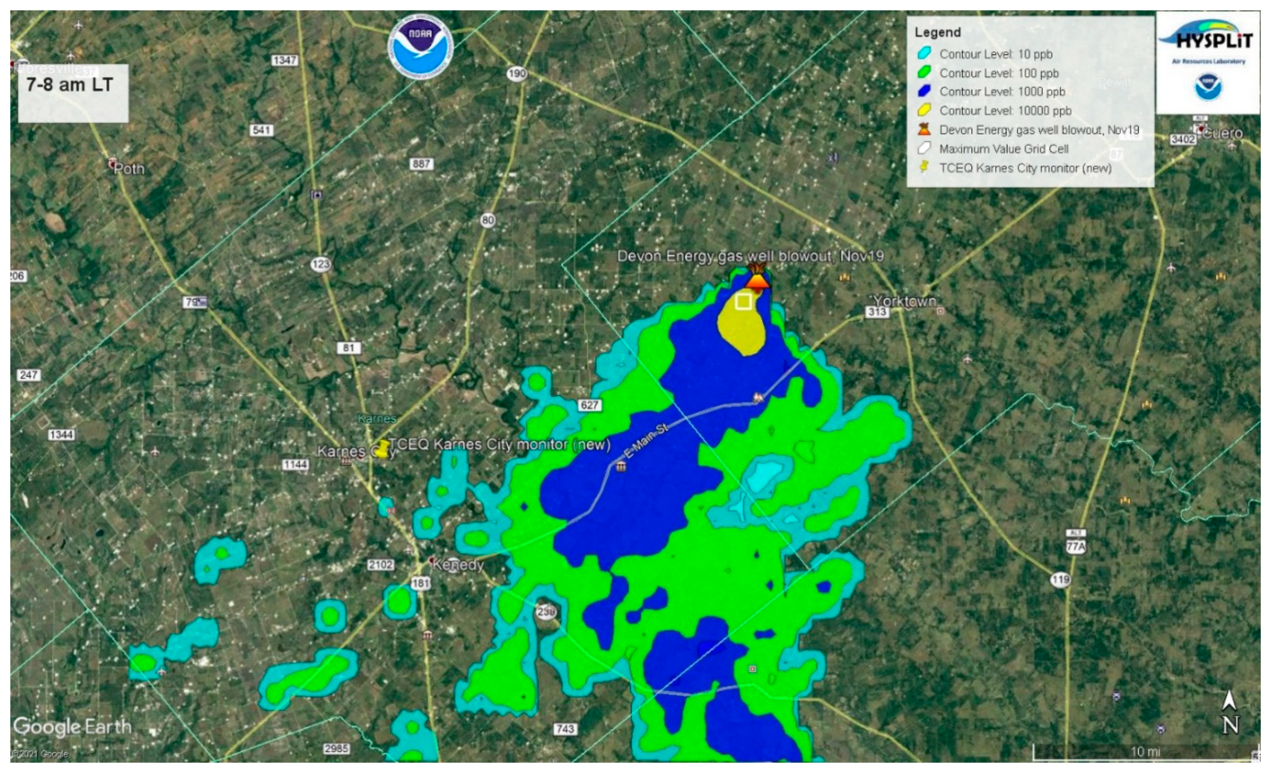
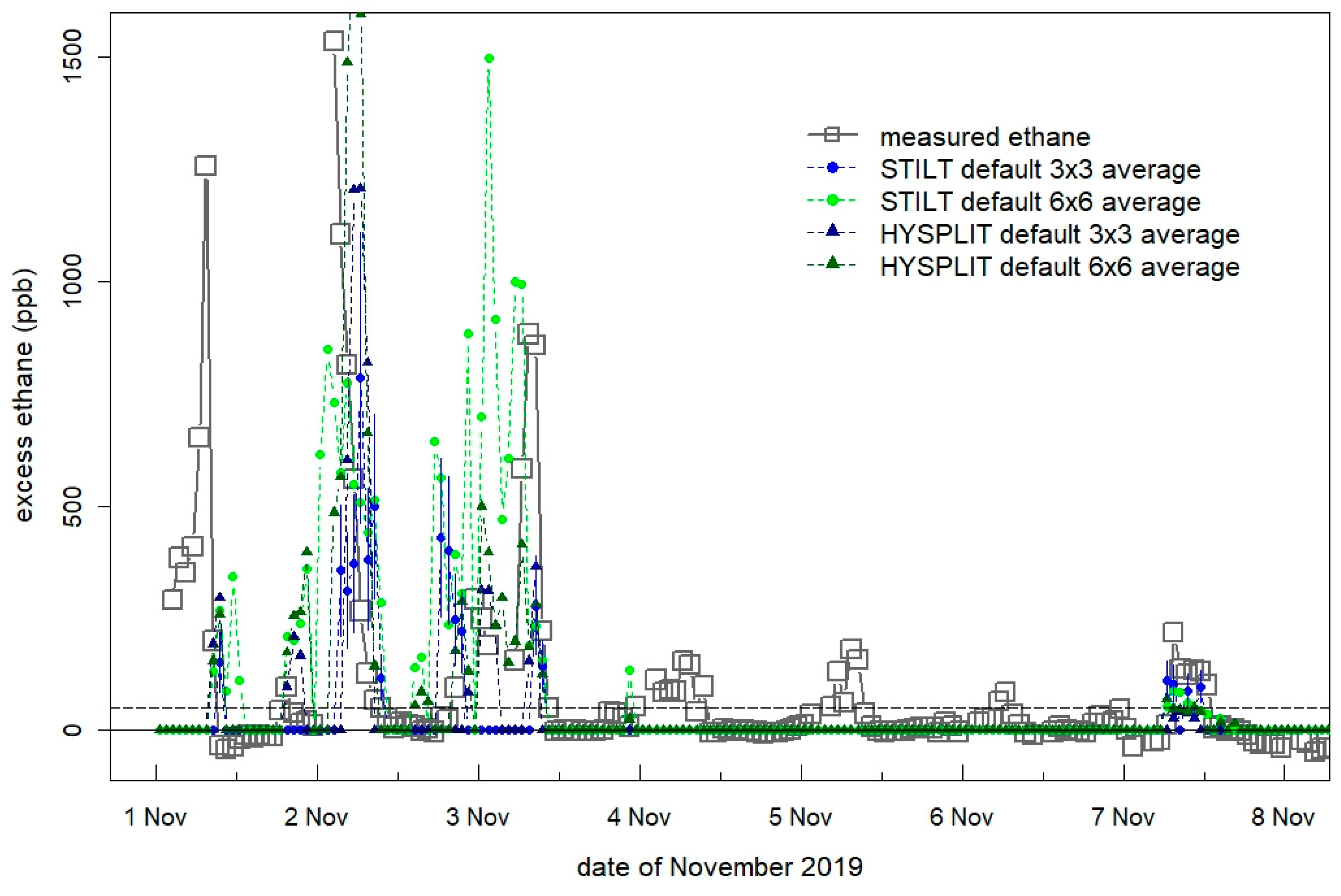
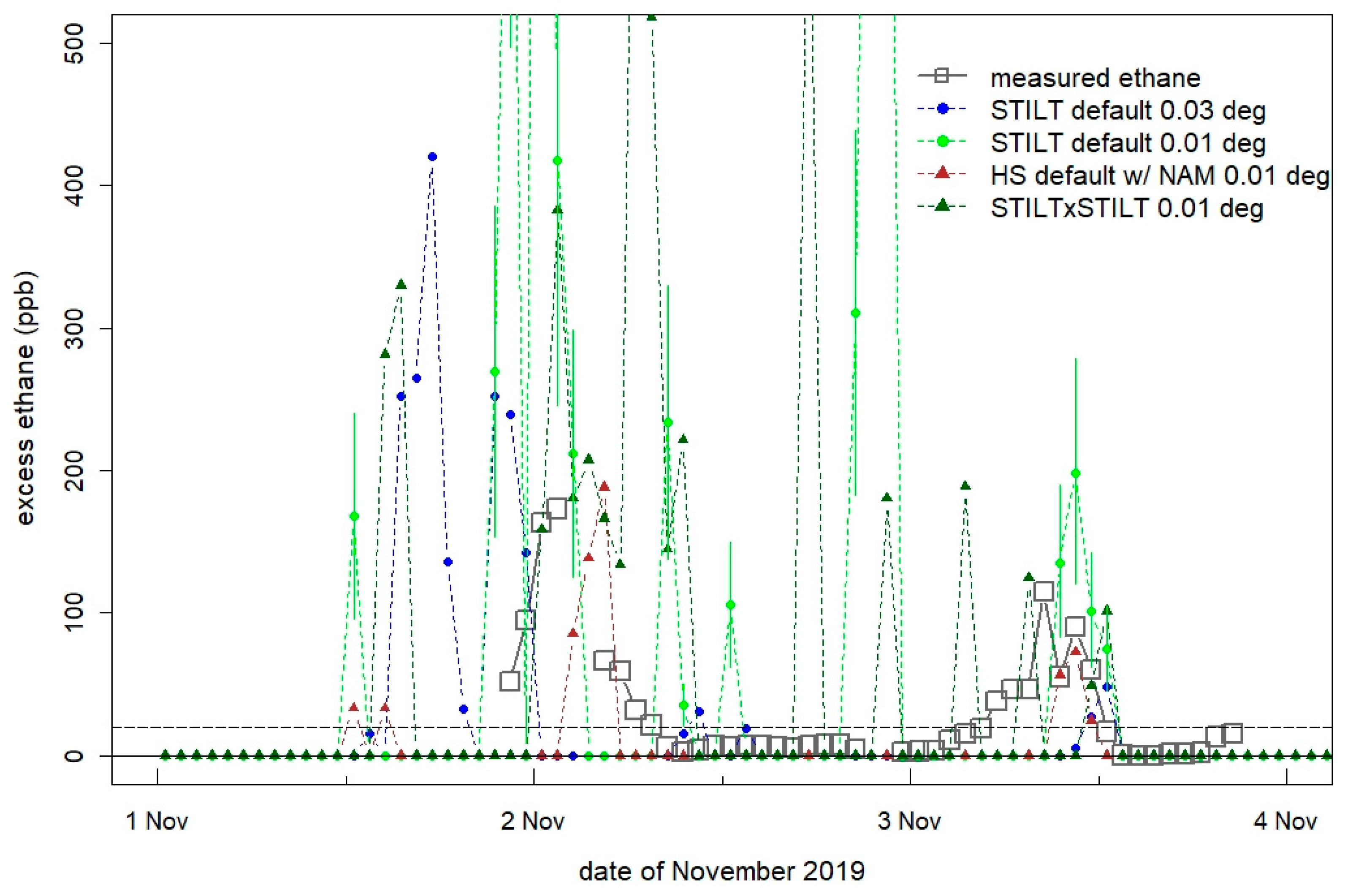
3.4. HYPLIT Model Results Compared to Air Quality Monitor Observations

We ran the PC version of HYSPLIT for all tests. Dispersion modeling was limited to 10 HRRR meteorology input files (the maximum is 12, aka 72 h). The model was initiated at midnight UTC, thus 6 pm local Texas standard time, and only data after 30 h into the run (midnight local time) was used for comparisons. A 3° × 3° domain around the blowout location was modeled, in most cases at a grid resolution of 0.01 degrees. The output file contained the average, hourly dilution ratio at levels below 50 m above ground. Gridded ASCII file output data was created from the main binary output file, and read into R software for further analysis. Google Earth output data (kmz-files) in the form of contours were created to view the results in spatial format overlaid on standard maps.
An example contour plot overlaid on a Google Earth map is shown in Figure 8. It depicts the extrapolated impact from the STILT × STILT 0.01 degree resolution run in the Dewitt and Karnes County areas downwind of the blowout during the morning hour of 7–8 am on 1 November 2019. As shown in Figure 4, ethane at the monitor was very high at this hour, but the blowout plume as calculated by HYSPLIT had not reached the monitor location yet, suggesting timing uncertainties in the meteorology during that period. While the maximum local ethane mixing ratio was observed between 7 and 8 am that morning, HYSPLIT calculated that it should have arrived 1–2 h later, and at >1000 ppb (blue shading in Figure 7). So while the timing was off in this example, the magnitude of impact at the receptor matched. Notably, HYSPLIT results indicated that the plume was north of the monitor after 11 am on that day, consistent with a lack of significant impact observed at that time.
A similar situation occurred on 2 November 2019. In that case as well, although HYSPLIT correctly indicated a major impact at the monitor in the early morning hours of 4–8 am, local measurements suggest that maximum impacts occurred 1–3 h earlier. We note that in both these examples, a calculation at higher resolution than the meteorological input data was selected, and the HYSPLIT program’s contour display routine was executed to create the kmz-files displayed. The program caries out two internal extrapolations for this: (i) it extrapolates the meteorological data linearly to the desired grid output resolution, and (ii) it extrapolates the gridded output data when creating the contour plots. This is reasonable and advantageous for on-screen displays and outreach to the media and citizens impacted by such emission events. However, for the analyses below, the gridded output data was directly compared to the monitor data for several grid averages. Namely, in the case of 0.01 × 0.01 degree resolution (approximately 1 × 1 km2), the center grid cell at the monitor, a 3 × 3 cell average, and a 6 × 6 cell average around the monitor were compared (see Figure 1). At the lower (native met model) 0.03 × 0.03 degree resolution (3 × 3 km2), the center grid cell at the monitor, and a 3 × 3 cell (9 × 9 km2) average were compared to the excess ethane data from the air quality monitor measurements.

3.4.1. Performance of HYSPLIT Evaluated for the Karnes City Monitor

A first look at the performance of HYSPLIT for this emission event is given in Figure 9 as a time series of excess ethane measurements and different model run forecasts for the first week of data, when emission rates were high enough to cause significant excess hydrocarbon observations. As illustrated, the timing offset described above is mostly eliminated when spatial averaging is used. Smaller impacts were missed by HYSPLIT on November 4–6, but correctly quantified on November 7. The major impacts at the Karnes City monitor on November 1–3 were at times under- or overestimated depending on day, hour, and spatial averaging choice. The STILT default method calculations produced slightly larger surface layer mixing ratios at coarser averaging, meaning the improved STILT dispersion calculation method implemented in HYSPLIT version 5.0 causes less vertical dilution as compared to the default HYSPLIT dispersion algorithm. Not shown in Figure 8 are any model outputs for the single 0.01 × 0.01 degree grid cell containing the monitor location, because in all cases those values were few and far apart, underestimating the measured impact due to spatial offsets. This suggests that higher than native met-model resolutions may not be meaningful unless post-run grid cell averaging is applied to the output, and for this mid-field distance comparison.
None of the other model runs not shown in Figure 9 (Table 1) showed substantially different results to the two runs depicted. Nevertheless, to compare the results against each other, we calculated a similar ranking metric as Loughner et al. [15] as follows:
R a n k = r 2 + ( 1 | F B 2 | ) + ( 1 K S )
In Equation (1), r2 is the determination coefficient of a linear correlation of integrated daily excess ethane mixing ratios (first ten days), which avoids timing offsets. FB is the normalized fractional bias, and KS is the Kolmogorov–Smirnov test statistic. For both FB and KS, hourly data was used, but only when measurements were available and the measured excess ethane exceeded 50 ppb (horizontal dashed line in Figure 9) to avoid random effects on ethane from other petrochemical emission sources than the blowout. The highest value for Rank is 3 (perfect model), the lowest 0 (no model skill).
We compared the standard, default HYSPLIT dispersion setup (using the Kanthar–Clayson vertical turbulence parametrization and met-model derived PBL depth) at 0.01 × 0.01 degree resolution (“HKC1”) against the otherwise identical STILT dispersion setup (“HS1”), the STILT dispersion setup with STILT parametrization (“HSS1”, using the Hanna vertical turbulence parametrization and a modified Richardson Number PBL depth calculation), the default HYSPLIT dispersion setup using NAM input data (“HKC1NAM”, 12 km resolution met data), and the STILT dispersion setup at native met-model resolution (“HS3”). Only the spatially averaged outputs were compared. The results are summarized in Table 3. Following Loughner et al. [15], differences in Rank of 0.1 or larger may be considered meaningful, meaning, are likely statistically significant.
It is apparent from Table 3 that using lower-resolution meteorological input data (such as the 12 km NAM) does not automatically lead to an overall lower performance in this test. There is also little difference in the standard STILT setup between higher resolution averaged to a 6 × 6 km area (HS1) and native resolution averaged to a 9 × 9 km area (HS3). Both belong to the highest-performing runs. While, for the event analyzed here, the standard HYSPLIT setup (HKC1) delivered slightly better results than the equivalent STILT version (HS1) when averaged over the central 9 grid cells (3 × 3 km2), the standard STILT version was superior at larger spatial averaging (HS1, 6 × 6 km2). Using the additional STILT model parameterizations (HSS1) improved the model at the finer spatial averaging, but not at the coarser spatial averaging.
When compared with respect to vertical dispersion characteristics, we found that the standard HYSPLIT scheme using the Kanthar–Clayson turbulence parametrization (HKC1) did not produce systematically lower concentrations in the boundary layer as compared to the STILT scheme using the Hanna parametrization (HSS1). On average, the former tended instead to deliver slightly higher near-surface ethane mixing ratios than the latter when averaged over the 3 × 3 km2 area around the receptor location (see also Figure 9). The two example hours shown in Figure 10 demonstrate the generally similar results between the model outputs, suggesting that the met-model input data may play a more prominent role than the parametrizations used in different model schemes.
Figure 11 shows a comparison of the integrated daily excess ethane mixing ratios, demonstrating the model’s skill at the 0.03 degree resolution across different setups. While HYSPLIT showed considerable skill in forecasting how the emissions event plume was dispersing downwind, this example demonstrates that impacts at this spatial resolution were generally underestimated by approximately a factor of two. As the emission rate related error bars on the HSS1 model indicate, this is very likely not related to an underestimation of the emissions. In turn, because larger spatial averaging improves this relationship, the underestimation is probably caused by uncertainties in the plume transport.
We note that all HYSPLIT model runs missed apparently significant impacts on 4–6 November 2019 under near continuous southeasterly winds. This may be explained by the variability of possible background levels we subtract from the observations based on known prior variability of ethane at the AQ monitoring location in the absence of a nearby blowout. Note from Figure 4 that interquartile ranges, but especially outlier conditions include ethane levels of up to 100–300 ppb during nighttime hours, comparable to the calculated excess levels above median values used to calculate the data in Figure 9 on 4–6 November. We can therefore not exclude the possibility that the excess levels shown in Figure 9 were simply lower during these days due to higher than median emissions from sources other than the blowout location.
We also note that the underestimations by the models, especially during the overnight hours on 1–3 November, cannot be reconciled with a lower than calculated emission rate, especially not a 3-fold lower emission rate as claimed by the well site operator. In addition, while the company first reported the blowout at 2 am local time on November 1, 2019, the data obviously indicate that emissions were already reaching the 30 km distant air quality monitor location at that time. Therefore, the onset of the blowout most likely occurred 6–12 h prior, and was thus modeled as such.

3.4.2. Performance of HYSPLIT Evaluated for the Floresville Hospital Monitor

The blowout emission plume was also encountered at the Floresville Hospital air quality monitor several times during the 20 days of the event. However, no data was available during several days of the first week (4–6 November 2019) when blowout emissions were highest. Thus, we focused our analyses on the first three days of the blowout when local data at the monitor showed significant impacts. Figure 12 shows the time series of excess ethane measurements and 3 × 3 km averaged model outputs, similar to Figure 9. Most model runs overestimated impacts at the monitor location during 1 and 2 November, but correctly captured impacts on 3 November 2019. While the default settings with STILT dispersion strongly overestimated the observations on 1 and 2 November, generally more moderate overestimations—except for four hours in the morning of the 2nd—occurred when using STILT dispersion with STILT parameterizations (STILT × STILT). In this example, the lower-resolution NAM input met data let to an overall good match.
Model performance is summarized in Table 4. Note, however, that these results are less robust compared to those shown in Table 3 because only three days with limited hours of comparison were available (n = 15; only including excess ethane measurements > 20 ppb for the Floresville location). The best performances were observed for the HSS1 model and the lower-resolution default HS3 model, when averaged over a larger area. Similar to the comparisons at the Karnes City monitor, the STILT dispersion model versions appeared to provide slightly better performances as compared to the default HYSPLIT dispersion runs.
It is illustrative to look at the plume position across models during 3 November 2019 when it was impacting the Floresville monitor during the morning hours, Figure 13. After overnight transport toward the southwest and south, strongly impacting the town of Nordheim just 7.5 km south of the blowout location, winds shifted to the east-southeast and moved emissions toward both monitors in the west-southwest (Karnes City) and west-northwest (Floresville) of the blowout. The example depicts the plume positions, calculated using STILT dispersion for various turbulence parametrizations, between 10 and 11 am local time. In all cases, impacts occurred at both monitors, as observed. However, while the Karnes City monitor was well inside the plume (green shading), the Floresville Hospital monitor was only affected at the edges of the plume (light blue shading) in all cases. It may thus come to no surprise that, regardless of the turbulence parametrization, the models were not able to quantify the impact’s magnitude consistently. In this situation, model results become sensitive to spatial averaging across the plume’s edge, and therefore uncertainties about impacts from the emissions event increase, especially when coarser met-model input data are used.

4. Conclusions

We found a very high likelihood that emissions from the 1 November 2019 gas well blowout in Dewitt County, Texas, reached two distant TCEQ air quality monitors during several distinct periods while the blowout was underway. Excess hydrocarbon ratios observed at the monitors were comparable to observations made near the blowout during the same period, and reflect a mixture of gas and condensate emissions from the field in question. Blowout hydrocarbon emissions were very likely much higher than reported by the responsible company, and we instead used satellite derived data for methane emissions alongside emission permit application informed methane-to-ethane ratios to derive ethane emissions data as inputs to dispersion modeling. We tested several HYSPLIT dispersion and turbulence parameterizations, using mostly high fidelity, 3 km-resolution HRRR meteorological input data, and some 12 km-resolution NAM data for comparison. HYSPLIT captured both the periods of most excess hydrocarbon impacts at the downwind air quality monitors, and quantified the daily integral impacts to within a factor of two under most circumstances. HYSPLIT hourly ethane concentration results did not reveal a consistent pattern of over- or underestimation when juxtaposed with calculated excess ethane at each monitor, derived by subtracting median background abundances under similar meteorological conditions that occurred in 2019. Both a lack of highly accurate emission rate data and confidently unbiased excess ethane measurement data, however, preclude us from judging which model setup is preferred for accurate emission event impact forecasting. Nevertheless, a calculated rank measure demonstrated that both the use of higher-resolution meteorological input data, and the use of the new STILT versus the standard HYSPLIT dispersion scheme, alongside appropriate downwind averaging of grid cells, produces satisfactory results.
We note that accurate input data on source emissions are critical to determine the model results’ fidelity (of forecasts) of the severity of downwind impacts. Our HYSPLIT modeling results confirm that the observed impacts of this emissions event would have been strongly underestimated if we had used the 3-fold lower hydrocarbon emission estimates reported by the company in charge of the blowout well. In addition, significant amounts of condensate emissions, including air toxics such as benzene, were emitted by the event, but not listed by the responsible operator. Local measurements within two kilo-meters of the blowout showed short-term benzene levels over 200 ppb, and 24 h averages of 10 ppb and higher. Based on the dispersion runs, both the nearby towns of Yorktown (10 km east) and Nordheim (7.5 km south) probably experienced near-surface benzene levels of 5–50 ppb during numerous nighttime hours during the first week of the blowout. That would often have been above the EPA’s Rfc value (inhalation reference concentration) of 9.4 ppb. Together with several other aromatic hydrocarbons emitted, the emissions event thus may have had non-negligible health effects on a significant part of the human population living in the area.

Author Contributions

Conceptualization, funding acquisition, project administration, methodology, data analysis, and writing—original draft preparation and editing, G.W.S.; data curation and analysis and writing—parts of original draft and review, M.L.G. All authors have read and agreed to the published version of the manuscript.

Funding

This research was partially funded by the Texas Air Research Center under project number 110TAM0183A in 2020.

Institutional Review Board Statement

Not applicable.

Informed Consent Statement

Not applicable.

Data Availability Statement

Data used for this project can be found in the Texas Data Repository at https://doi.org/10.18738/T8/MK4M3V (accessed 14 March 2022). Air quality monitoring data from the AQ stations evaluated can be found at https://www.tceq.texas.gov/cgi-bin/compliance/monops/agc_daily_summary.pl (accessed 14 March 2022).

Acknowledgments

The authors gratefully acknowledge the NOAA Air Resources Laboratory (ARL) for the provision of the HYSPLIT transport and dispersion model. We also thank the employees at the Texas Commission on Environmental Quality (TCEQ) for providing (i) non-public measurement data near the blowout site, (ii) the TCEQ’s blowout report, and (iii) information about local oil and gas well emission permit data and its interpretation.

Conflicts of Interest

The authors declare no conflict of interest.

References

  1. Ngan, F.; Loughner, C.P.; Stein, A. The evaluation of mixing methods in HYSPLIT using measurements from controlled tracer experiments. Atmos. Environ. 2019, 219, 117043. [Google Scholar] [CrossRef]
  2. Karion, A.; Lauvaux, T.; Coto, I.L.; Sweeney, C.; Mueller, K.; Gourdji, S.; Angevine, W.; Barkley, Z.; Deng, A.J.; Andrews, A.; et al. Intercomparison of atmospheric trace gas dispersion models: Barnett Shale case study. Atmos. Chem. Phys. 2019, 19, 2561–2576. [Google Scholar] [CrossRef] [PubMed] [Green Version]
  3. Ionov, D.; Poberovskii, A. Observations of urban NOx plume dispersion using mobile and satellite DOAS measurements around the megacity of St. Petersburg (Russia). Int. J. Remote Sens. 2019, 40, 719–733. [Google Scholar] [CrossRef]
  4. Castro, M.; Pires, J.C.M. Decision support tool to improve the spatial distribution of air quality monitoring sites. Atmos. Pollut. Res. 2019, 10, 827–834. [Google Scholar] [CrossRef]
  5. Pirouzmand, A.; Kowsar, Z.; Dehghani, P. Atmospheric dispersion assessment of radioactive materials during severe accident conditions for Bushehr nuclear power plant using HYSPLIT code. Prog. Nuclear Energy 2018, 108, 169–178. [Google Scholar] [CrossRef]
  6. Ngan, F.; Stein, A.; Finn, D.; Eckman, R. Dispersion simulations using HYSPLIT for the Sagebrush Tracer Experiment. Atmos. Environ. 2018, 186, 18–31. [Google Scholar] [CrossRef]
  7. Fasoli, B.; Lin, J.C.; Bowling, D.R.; Mitchell, L.; Mendoza, D. Simulating atmospheric tracer concentrations for spatially distributed receptors: Updates to the Stochastic Time-Inverted Lagrangian Transport model’s R interface (STILT-R version 2). Geosci. Model. Dev. 2018, 11, 2813–2824. [Google Scholar] [CrossRef] [Green Version]
  8. Duc, H.N.; Chang, L.T.C.; Azzi, M.; Jiang, N.B. Smoke aerosols dispersion and transport from the 2013 New South Wales (Australia) bushfires. Environ. Monit. Assess. 2018, 190, 1–22. [Google Scholar] [CrossRef] [PubMed]
  9. Rolph, G.; Stein, A.; Stunder, B. Real-time Environmental Applications and Display System: READY. Environ. Model. Softw. 2017, 95, 210–228. [Google Scholar] [CrossRef]
  10. Truong, S.C.H.; Lee, M.I.; Kim, G.; Kim, D.; Park, J.H.; Choi, S.D.; Cho, G.H. Accidental benzene release risk assessment in an urban area using an atmospheric dispersion model. Atmos. Environ. 2016, 144, 146–159. [Google Scholar] [CrossRef] [Green Version]
  11. Stein, A.F.; Ngan, F.; Draxler, R.R.; Chai, T. Potential Use of Transport and Dispersion Model Ensembles for Forecasting Applications. Weather Forecast 2015, 30, 639–655. [Google Scholar] [CrossRef]
  12. Stein, A.F.; Draxler, R.R.; Rolph, G.D.; Stunder, B.J.B.; Cohen, M.D.; Ngan, F. NOAA’s HYSPLIT Atmospheric Transport and Dispersion Modeling System. Bull. Am. Meteorol. Soc. 2015, 96, 2059–2077. [Google Scholar] [CrossRef]
  13. Ngan, F.; Stein, A.; Draxler, R. Inline Coupling of WRF-HYSPLIT: Model Development and Evaluation Using Tracer Experiments. J. Appl. Meteorol. Climatol. 2015, 54, 1162–1176. [Google Scholar] [CrossRef]
  14. Lin, J.C.; Gerbig, C.; Wofsy, S.C.; Andrews, A.E.; Daube, B.C.; Davis, K.J.; Grainger, C.A. A near-field tool for simulating the upstream influence of atmospheric observations: The Stochastic Time-Inverted Lagrangian Transport (STILT) model. J. Geophys. Res. Atmos. 2003, 108, 4493. [Google Scholar] [CrossRef] [Green Version]
  15. Loughner, C.P.; Fasoli, B.; Stein, A.F.; Lin, J.C. Incorporating Features from the Stochastic Time-Inverted Lagrangian Transport (STILT) Model into the Hybrid Single-Particle Lagrangian Integrated Trajectory (HYSPLIT) Model: A Unified Dispersion Model for Time-Forward and Time-Reversed Applications. J. Appl. Meteorol. Climatol. 2021, 60, 799–810. [Google Scholar] [CrossRef]
  16. Hegarty, J.; Draxler, R.R.; Stein, A.F.; Brioude, J.; Mountain, M.; Eluszkiewicz, J.; Nehrkorn, T.; Ngan, F.; Andrews, A. Evaluation of Lagrangian Particle Dispersion Models with Measurements from Controlled Tracer Releases. J. Appl. Meteorol. Climatol. 2013, 52, 2623–2637. [Google Scholar] [CrossRef]
  17. R Core Team. R: A Language and Environment for Statistical Computing; R Foundation for Statistical Computing: Vienna, Austria, 2020; Available online: https://www.R-project.org/ (accessed on 14 March 2022).
  18. Cusworth, D.H.; Duren, R.M.; Thorpe, A.K.; Pandey, S.; Maasakkers, J.D.; Aben, I.; Jervis, D.; Varon, D.J.; Jacob, D.J.; Randles, C.A.; et al. Multisatellite Imaging of a Gas Well Blowout Enables Quantification of Total Methane Emissions. Geophys. Res. Lett. 2021, 48, e2020GL090864. [Google Scholar] [CrossRef]
Figure 1. Google Earth map of the study area (inset showing location within Texas). Note that the bright patches throughout the picture mark oil and gas well pad locations. The blowout location, a pad site next to Cotton Patch Rd. in Dewitt County, north of the town of Nordheim, TX [18], is marked on the upper right, while the main receptor location in southeast Karnes City, TX, a TCEQ air quality monitoring site, is marked on the lower left. The straight line in black indicates a 30 km travel distance for the emissions. The three boxes in yellow, red, and blue indicate 1, 3, and 6 km averaging areas, respectively, for the model’s gridded outputs.
Atmosphere 13 00486 g001
Figure 2. Modeled blowout location methane emissions in metric tons per hour from 1 to 20 November 2019 (black solid (mean) and dashed (95% conf. interval) lines from linear regression of log-transformed data; red line from non-linear regression). Note that flaring of hydrocarbons began on 14 November (350 h on this scale). Except for 1 November 2019 (see text), filled circles represent satellite estimates, and open circles represent Oil Climate Index (OCI) model-based estimates [18].
Atmosphere 13 00486 g002
Figure 3. Time series of hourly air temperature (red) and winds (black) from 31 October to 16 November 2019 from the Karnes City AQ monitor. Green dashed lines separate periods with similar meteorology.
Atmosphere 13 00486 g003
Figure 4. Diurnal development of ethane levels at the Karnes City AQ monitor in period 1 (lighter red is 1 November). The boxplot shows the calculated reference levels; green data points show ethane from the day prior to the blowout discovery around the midnight hours of 31 October to 1 November, and red data points show ethane from the two days thereafter.
Atmosphere 13 00486 g004
Figure 5. Time series (1–15 November 2019, 12 = midday on 1 November) of excess ethane mixing ratios at both TCEQ air quality monitoring sites. Dashed horizontal lines mark levels below which excess ethane may be insignificant (50 ppb for Karnes City, 20 ppb for Floresville) based on other, randomly occurring regional emissions.
Atmosphere 13 00486 g005
Figure 6. Example weather station to HRRR data comparison for a site in Texas approximately 60 km from the blowout location. (a) shows a scatter plot of one week of air temperature data, (b) shows one week of wind direction data from both datasets.
Atmosphere 13 00486 g006
Figure 7. Example excess hydrocarbon mixing ratio correlations at the air quality monitors investigated (1–3 November 2019), showing a high consistency between the ambient excess hydrocarbon observations.
Atmosphere 13 00486 g007
Figure 8. HYSPLIT kml file output for the ethane plume location integrated for 7–8 am LT, 1 November 2019. Near blowout, ethane levels would have exceeded 10 ppm (yellow shading and white square), while the monitor location in Karnes City had not been reached yet, but was an hour later.
Atmosphere 13 00486 g008
Figure 9. Time series of measured vs. modeled (0.01 deg. resolution) excess ethane mixing ratios at the Karnes City AQ monitor for two model setups and two spatial averaging alternatives (Figure 1). One model run includes error bars (STILT default 3 × 3, filled blue circles) illustrating emission rate uncertainties.
Atmosphere 13 00486 g009
Figure 10. Receptor location (Karnes City) excess ethane mixing ratio vertical distributions during two hourly periods (local time) of the early November impacts of the hydrocarbon plume. The vertical levels represent the height above ground over which the model results were averaged: 50 m = surface level (0–50 m), 100 m = 50–100 m level, 200 m = 100–200 m level, and so on.
Atmosphere 13 00486 g010
Figure 11. Scatter plot of integrated daily (sum of all 24 h alleviating timing offsets) excess ethane mixing ratios at the receptor site averaged to 0.03 degrees. Dashed and dotted lines represent correctly estimated, and factor-two underestimated integrated daily model results, respectively.
Atmosphere 13 00486 g011
Figure 12. Time series of measured vs. modeled (all 3 × 3 km averages) excess ethane mixing ratios at the Floresville Hospital monitor for several model setups (Table 1). One model run includes errors bars (STILT default 3 × 3, filled green circles) illustrating emission rate derived uncertainties. The dashed horizontal line marks excess ethane mixing ratios (<20 ppb) that may have arisen from random emissions other than the blowout at 54 km from the monitor.
Atmosphere 13 00486 g012
Figure 13. HYSPLIT-program plotted 3 November 2019, 10–11 am LT, blowout emission plume positions using STILT dispersion with four different turbulence parametrizations: Hanna = Hanna, K-C = Kanthar–Clayson, met-mod = meteorological model’s TKE field, B-H = Beljaars/Holtslag turbulence parametrization. The star marks the blowout location, and the two orange dots mark the air quality monitor locations, the closer one being the Karnes City monitor.
Atmosphere 13 00486 g013
Table 1. HYSPLIT dispersion model runs used in this project.
Method (Abbreviation)Met InputResolution 1Processing Time 2
STILT default (HS1)HRRR 3 km0.01 deg (1 km)525 ± 153
STILT default (HS3)HRRR 3 km0.03 deg (3 km)383 ± 186
HYSPLIT default (HKC1)HRRR 3 km0.01 deg (1 km)248 ± 122
HYSPLIT default (HKC3)HRRR 3 km0.03 deg (3 km)251 ± 89
HYSPLIT default (HKC1NAM)NAM 12 km0.01 deg (1 km)180 ± 42
STILT × STILT (HSS1) 3HRRR 3 km0.01 deg (1 km)539 ± 166
1 Resolution refers to the output resolution of the model, e.g., a 0.01 deg., or 1 km output grid is thus at higher resolution than the native resolution of the meteorological input data, and is achieved within the HYSPLIT program via interpolation of the coarser data to the finer grid. 2 Processing times are the average (±1 sd) length in seconds for 54 h model runs on a standard PC (Intel i7, 3.6 GHz, 16 Gb RAM, 64-bit Win10) for the 20 days analyzed (1–20 November 2019). 3 STILT dispersion plus new STILT vertical turbulence setting (Hanna boundary layer turbulence parameterization, see Loughner et al., 2021 [15] and Section 4.3.1).
Table 2. Observed hydrocarbon ratios in permit applications, near the blowout, and as determined from Karnes City and Floresville air quality monitor data.
CompositionGas OnlyWell-StreamAmbientAmbientAmbient
origin2017 permit2009 wildcatblowoutKarnes CityFloresville
C3/C2 10.380.48NA0.630.59
nC4/C30.280.4NA0.490.49
iC4/nC40.70.65NA0.490.46
totC5/totC40.340.560.4330.490.54
benz/totC40.005NA0.0310.0090.012
tol/totC40.012NA0.1470.020.03
benz/tol0.42NA0.210.27–0.4 20.31
1 C2 = ethane, C3 = propane, nC4 = n-butane, iC4 = isobutane, totC4 = nC4 + iC4, totC5 = n-pentane + isopentane, benz = benzene, and tol = toluene. 2 Inconsistent slope (see Figure 7).
Table 3. Model performance Rank by setup and spatial average.
Spatial AverageHS1 1HS3HKC1HKC1NAMHSS1
3 × 3 km1.110.901.271.221.24
6 × 6 km1.841.78 21.591.341.61
1 See text and Table 1 for model abbreviation explanation. 2 9 × 9 km output.
Table 4. Model performance Rank by setup and spatial average.
Spatial AverageHS1 1HS3HKC1HKC1NAMHSS1
3 × 3 km1.690.481.141.421.99
6 × 6 km1.401.93 21.301.612.40
1 See text and Table 1 for model abbreviation explanation. 2 9 × 9 km output.
Publisher’s Note: MDPI stays neutral with regard to jurisdictional claims in published maps and institutional affiliations.

