1. Introduction
Visibility (VIS) is an important indicator of the transmittance of the atmosphere. In the recent 10 years, China has experienced many severe haze and fog events which are often accompanied by extremely low visibility and high PM
2.5 concentrations due to rapid urbanization and industrialization [
1,
2,
3,
4,
5,
6,
7]. Low visibility conditions present a host of problems of people’s daily activities and have become a major concern in air pollution studies and climatology [
8,
9,
10,
11,
12,
13,
14].
Atmospheric visibility in winter is closely related to the direct extinction of aerosols and water vapor [
15,
16,
17,
18]. Previous studies have revealed that aerosol particles, especially PM
2.5, have a strong attenuation effect on visibility through the direct effect of absorbing and scattering solar radiation [
15,
19], and the scattering of solar radiation by aerosol particles is highly dependent on RH, as hygroscopic particles take up water with increasing RH [
20,
21,
22,
23,
24]. Moreover, the direct extinction of fog droplets under the near saturation of water vapor is the other key factor of visibility degradation [
21,
24]. Both high PM
2.5 concentration and high RH can result in the occurrence of low visibility [
6,
25]. The key point of low visibility calculation and prediction depends on reasonable understanding of the correlation between visibility, PM
2.5 concentration, and RH.
In order to increase the safety and efficiency of transportation under low visibility conditions, developing parameterization schemes of low visibility is necessary for low visibility forecasts and numerical calculations. The parameterization methods of visibility could be roughly divided into four categories [
26,
27,
28,
29]. The empirical equation from IMPROVE (Interagency Monitoring of Protected Visual Environments) reconstructs the relationship between the mass concentration of chemical components of aerosol particles and the extinction coefficient [
27,
30,
31]. The Mie model calculates the optical parameters of spherical particles based on the corresponding particle number size distribution and the complex refractive index [
26,
28,
32]. The third parameterization of light extinction is based on visibility, RH, aerosol hygroscopic growth factors, and particle number size distributions measured during the Haze in China [
33,
34]. The physical meaning of this method is relatively clear, and it has been proved to be suitable for some regions in China such as the Beijing-Tianjin-Hebei region and the Yangtze River Delta region [
26,
34]. The above three methods are developed based on the contribution of chemical characteristics of different aerosol components to the extinction coefficient. However, because of the uncertainty of aerosol hygroscopic growth factor under high humidity conditions, these schemes usually overestimated low visibility below 5 km [
25,
26]. The spatiotemporal distribution difference of aerosol species also limits their applicability in China. The visibility statistical algorithm establishes a regression equation of visibility or extinction coefficient and its influencing factors, including the concentrations of PM, such as PM
10 and PM
2.5, and their chemical components, ozone gaseous pollutants, such as sulfur dioxide and nitrogen dioxide, and meteorological conditions, such as RH, wind speed, temperature, and boundary layer height [
29,
35,
36,
37,
38,
39]. For example, Zhou et al. [
29] established a multiple regression equation of visibility, PM
2.5 concentration, 10 m wind speed, wind shear (500–850 hPa), RH, temperature difference (925–1000 hPa), and potential pseudo-equivalent temperature difference (850–925 hPa) in Yangtze River Delta (YRD). This equation predicted the visibility variations during the winter of 2014–2015 well, with a correlation coefficient of 0.77. Jiang et al. [
26] compared the fitting visibility in Lin’an calculated by different regression methods, which was developed based on visibility, PM
2.5, PM
10, and RH [
35,
40], and the R
2 values between observations and calculations were 0.32–0.88. However, the common problem of these visibility parameterization schemes is their low efficiency on low visibility (VIS <5 and 3 km) prediction in winter [
25,
29]. In this study, new multivariate nonlinear regression equations of low visibility focusing on severe haze–fog pollution in eight regions of China are proposed.
Here, using the observations from December 2016 to February 2017, the relative contribution differences of PM
2.5 concentrations and RH changes to visibility reduction in the eight regions of China (
Figure 1a) are investigated in depth. Considering these differences, the data sets of the eight regions are grouped by different RH levels (BTH, GZP, and NEC: RH < 80%, 80% ≤ RH < 90% and RH ≥ 90%; CC, SCB, YRD, and SCC: RH < 85%, 85% ≤ RH < 95% and RH ≥ 95%; XJ: RH < 90% and RH ≥ 90%). Based on these RH groupings, new multivariate nonlinear regression equations of PM
2.5 concentration and humidity on visibility of the eight regions are established, respectively, and the low visibility forecasting capability (VIS < 5 and 3 km) of these new equations is evaluated based on the observations in January 2016–2020.
2. Data and Methodology
2.1. Data
The observation data used in this study include the ground-level meteorological factors and PM2.5 concentration and cover the January of 2016–2020, February of 2017, and December of 2016. MICAPS meteorological data, including visibility (VIS, km), temperature (T, °C), dew-point temperature (Td, °C) and present weather phenomena at 02:00, 05:00, 08:00, 11:00, 14:00, 17:00, 20:00, and 23:00 BJT, were obtained from the 654 sites of the China Meteorological Information Center. The RH (%) and Temperature dew point difference (T-Td, °C) values are calculated from T and Td. Hourly PM2.5 concentrations are provided by the 1496 stations of China National Environmental Monitoring Center. Extreme weather phenomenon, including precipitation, sand and dust could also lead to the occurrence of low visibility events. Therefore, the observation data under extreme weather conditions is eliminated.
Reanalysis of meteorological data, including the geopotential height (dagpm), temperature (T, K) u and v (components of the wind field, m s
−1) at heights of 500 and 850 hPa were obtained from the Modern-Era Retrospective Analysis for Research and Applications, Version 2 reanalysis meteorological data [
41]. These data have a spatial resolution of 0.5° × 0.5° and cover the same period as those of the observation data.
2.2. Statistical Analysis Method
This work mainly uses the regression analysis method. The regression equations between 3-hourly visibility and PM2.5 concentrations under different RH levels during the winter of 2016–2017 (December 2016 to February 2017) were calculated to analyze the relationship between visibility, PM2.5 concentration, and ambient humidity. Considering the contribution differences of changes in PM2.5 concentration and humidity to visibility reduction, the 3-hourly data sets of the eight regions are grouped by different RH levels (BTH, GZP, and NEC: RH < 80%, 80 ≤ RH < 90% and RH ≥ 90%; CC, SCB, YRD, and SCC: RH < 85%, 85 ≤ RH < 95% and RH ≥ 95%; XJ: RH < 90% and RH ≥ 90%). Most sensors for measuring humidity have an uncertainty or systematic error. Therefore, it is considered that ambient humidity reaches saturation when the RH increases to >95% in this paper. Using these RH grouping methods, new multivariate nonlinear regression equations of PM2.5 concentration and humidity (represented by T and Td) on visibility of the eight regions are established. The calculated visibility in January 2016–2020 (except 2017), which was calculated by these visibility regression equations, are compared with the observations to evaluate the visibility forecasting capability of this visibility statistical algorithm.
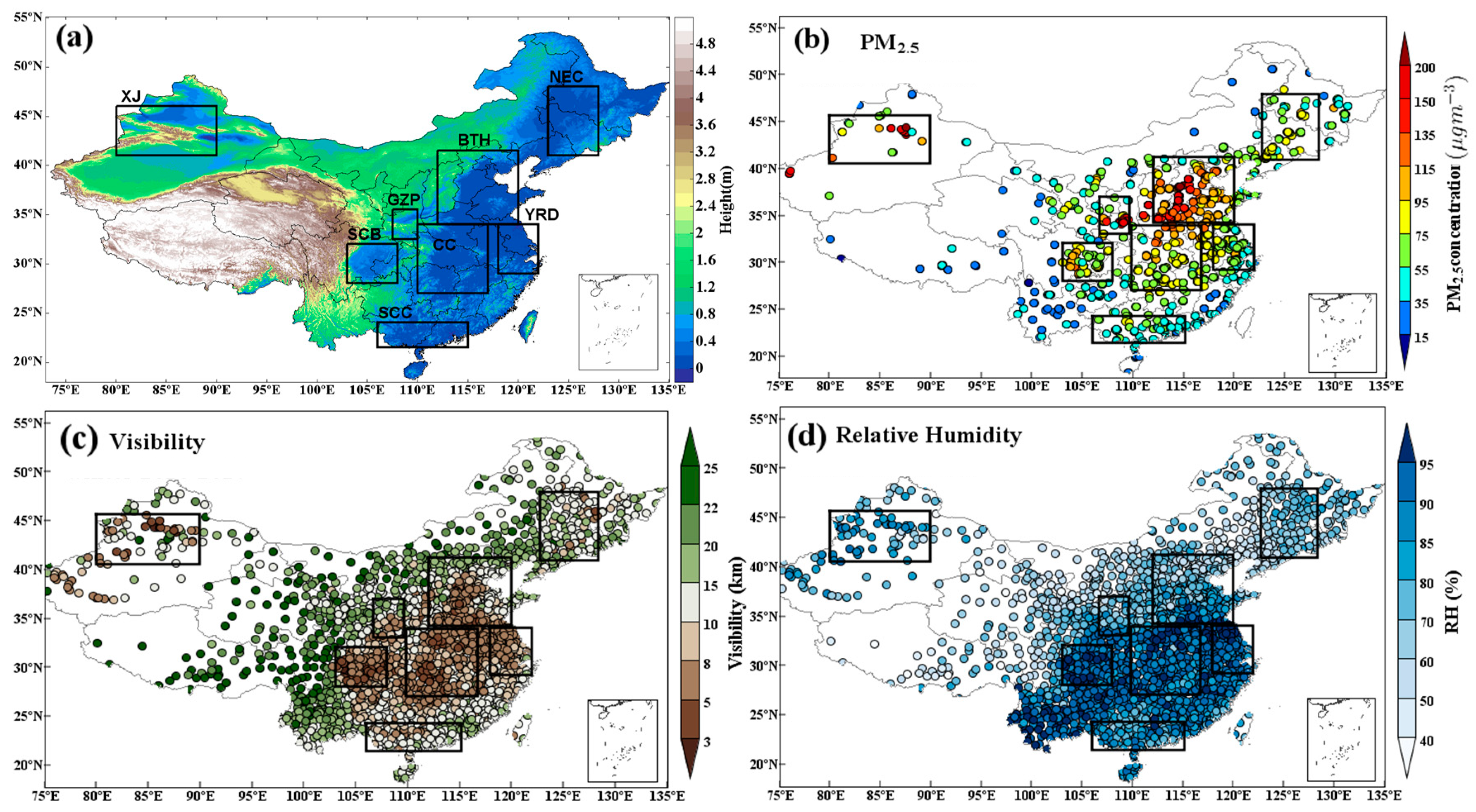
2.3. Regional Division
According to China’s climate regionalization scheme [
42], also considering the spatial distribution of the PM
2.5 observation stations (
Figure 1b) and ground meteorology stations (
Figure 1c,d), China is divided into the following eight regions in this study (
Figure 1a): Beijing-Tianjin-Hebei and its surrounding regions (BTH, 112° E–120° E, 34° N–41.5° N), Central China (CC, 110° E–117° E, 29° N–34° N), Guanzhong Plain (GZP, 107.5° E–110° E, 32.5° N–35.5° N), North Eastern China (NEC, 123° E–128° E, 41° N–48° N), Sichuan Basin (SCB, 103° E–108° E, 28° N–32° N), South China Coastal (SCC, 106° E–115° E, 21.5° N–24° N), Yangtze River Delta (YRD, 118° E–122° E, 29° N–34° N), and Xinjiang (XJ, 80° E–90° E, 41° N–48° N). The number of meteorology sites, PM
2.5 sites, and the total number of samples used in this study are listed in
Table 1.
3. Results and Discussion
3.1. Regional Distribution Differences of Winter Visibility, RH and PM2.5 Concentrations
Severe low visibility events were observed in many areas of China during the winter of 2016–2017 [
20,
43]. The spatial distribution of average visibility, PM
2.5 concentrations, and RH during this period is shown in
Figure 1. It is clear that low visibility is mainly located in the central and eastern parts of China, including BTH, CC, GZP, SCB, and YRD (
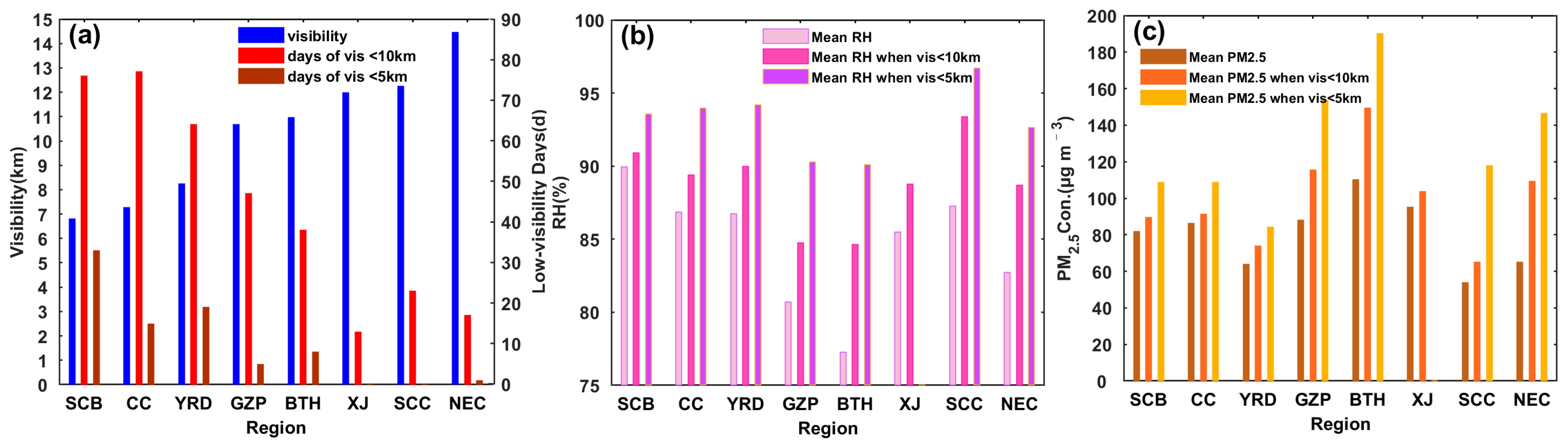
Figure 1c). The average visibility of the five regions ranked from low to high is SCB, CC, YRD, GZP, and BTH, respectively (
Figure 2a). The lowest visibility is found in SCB (6.8 km), which is located in Southwest China. The counts of daily mean visibility of less than 10 and 5 km are 76 and 33 d, accounting for 84% and 37% of the study period, respectively. The average RH of the five regions ranked from high to low is SCB (90.0%), CC (86.9%), YRD (86.7%), GZP (80.7%), and BTH (77.3%) respectively (
Figure 2b), which is consistent with the ascending order of visibility, suggesting that the higher the RH is, the lower the visibility is. Moreover, the mean RH under visibility <10 km in CC, SCB, and YRD is 89.6–90.9% and that under visibility <5 km is 93.5–94.2%. Mean RH under visibility <10 km in BTH and GZP is 84.6% and 86.8% and that under visibility <5 km is 90.0% and 90.3%, respectively. This also suggests the close relationship between low visibility (<5 km) and high RH (>90%).
The distribution of PM
2.5 concentrations in China also has obvious regional differences. As can be seen in
Figure 2c, the highest PM
2.5 concentrations are mainly observed in BTH and GZP. Many stations report PM
2.5 concentrations >150 μg m
−3, which represent heavy pollution according to the National Ambient Air Quality Standard in China (NAAQS). Therefore, even though the average RH in BTH and GZP is relatively lower, visibility <5 km is also observed because of the high aerosol loading. In addition, mean PM
2.5 concentrations under visibility <10 and 5 km in BTH, GZP, and NEC are 103.6–140.9 and 146.4–190.0 μg m
−3, 31.3–67.8 % and 72.7–124.5 higher than the average values. Mean PM
2.5 concentrations under visibility <10 and 5 km in CC, SCB, and YRD are 73.9–91.2 and 84.2–108.8 μg m
−3, 5.8–15.6 and 25.5–33.1% higher than the average values. PM
2.5 concentrations under low visibility conditions in BTH, GZP, and NEC are much higher than those in CC, SCB, and YRD. When visibility decreases from 10 to 5 km, the growth rates of PM
2.5 concentration in BTH, GZP, and NEC are also far higher than that of other regions. It suggests that the contribution of PM
2.5 concentration increase to visibility degradation in BTH, GZP, and NEC is probably higher than that of other regions.
The influence of PM2.5 concentrations and RH on visibility variations has obvious regional differences. Consequently, the relative contribution differences of changes in PM2.5 concentrations and RH to variations in visibility of the eight regions deserves further study.
3.2. Relative Contribution Differences of PM2.5 Concentrations and RH to Visibility Degradation
The concentrations of fine particulate and atmospheric humidity are the key factors affecting winter visibility in China [
44,
45,
46,
47,
48,
49,
50,
51]. T-T
d is often used to analyze ambient humidity. The smaller the value is, the higher the ambient humidity is. A value <5 °C is often considered as the necessary humidity condition for the occurrence of fog events.
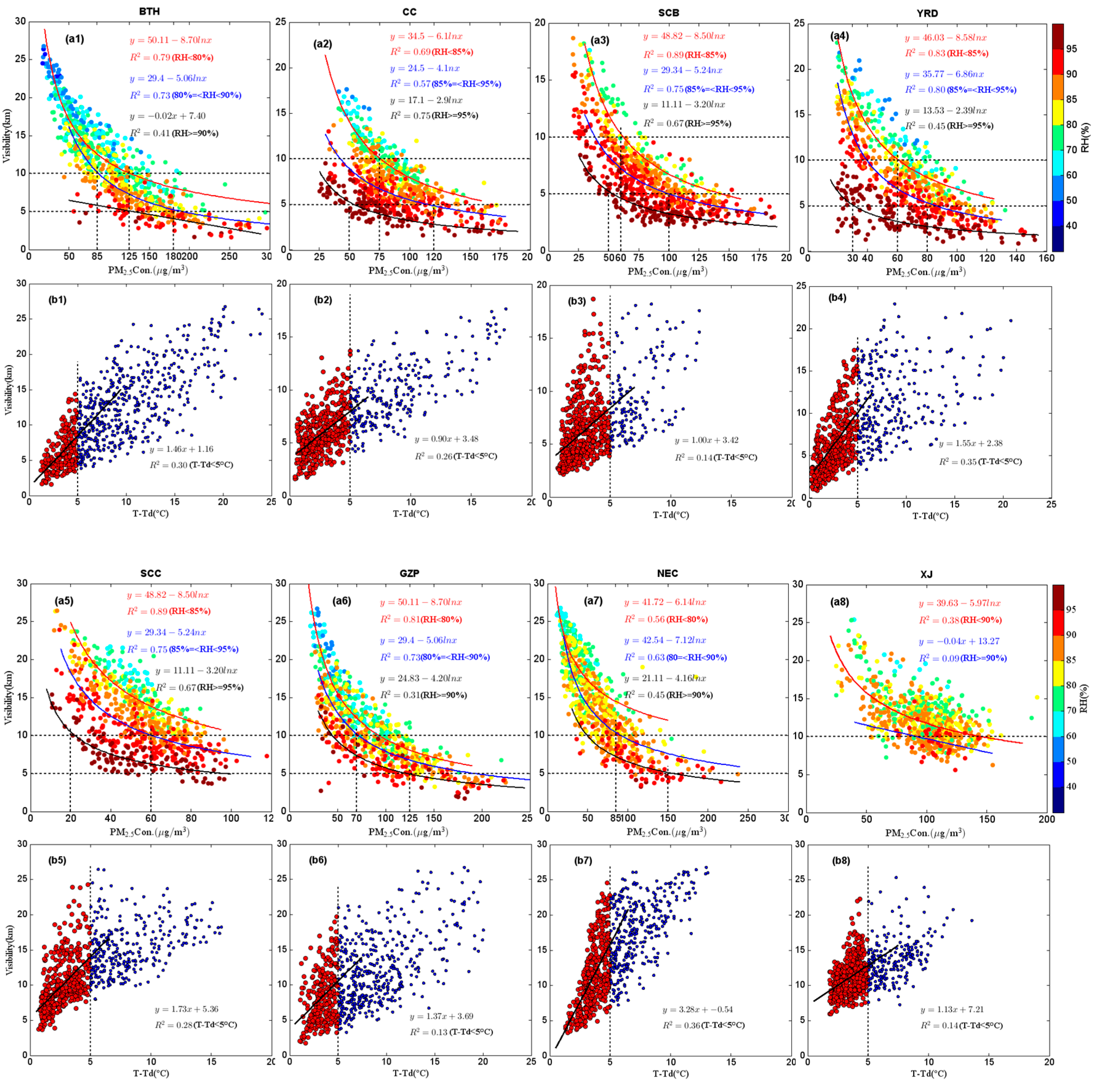
Figure 3 shows the scatter distributions of visibility, PM
2.5 concentrations, and T-T
d in the eight regions. It can be seen that the fitting relationships of PM
2.5 concentrations and visibility are significantly different with the increase in RH levels. Also considering the regional difference in RH distribution (
Figure 2b), the data groups of regions with relatively low RH (BTH, GZP, and NEC) are divided into three groups: RH < 80%, 80 ≤ RH < 90% and RH ≥ 90%, the data groups of regions with high RH (CC, SCB, SCC, and YRD) are divided into RH < 85%, 85 ≤ RH < 95% and RH ≥ 95%, respectively, and data groups of XJ are divided into RH < 90% and RH ≥ 90%. The relative contribution differences of changes in PM
2.5 concentration and RH to visibility decrease as well as their regional differences are investigated based on these RH grouping methods.
For BTH (
Figure 3(a1)) and GZP (
Figure 3(a2)), when the RH is <80% and PM
2.5 concentration is lower than <125 and 90 μg m
−3, respectively, the visibility in the two regions is usually >10 km. Within this range, the visibility decreases logarithmically with the PM
2.5 concentration increase. PM
2.5 concentration dominates the visibility changes while variation in RH contributes less. Both the continuous increase in PM
2.5 concentrations and RH lead to a further decrease in visibility to 10–5 km. With the RH increase to >80%, the correlation between PM
2.5 concentrations and visibility is weakened, and the contribution of RH becomes increasingly important. When the ambient RH increases to 80–90% and PM
2.5 concentration rises to >180 μg m
−3, the visibility of the two regions further drops to < 5 km. It is worth noting that as the RH further increases to >90%, PM
2.5 concentration >125 μg m
−3 could also result in visibility decreasing to <5 km, which is mainly caused by the strong hygroscopic growth of some aerosol particles with high water absorption (sulfate, nitrate, ammonium salt, and some soluble organic aerosols) [
22,
23,
24,
51,
52,
53,
54,
55,
56]. When the water vapor in the air is nearly saturated (RH > 95%), the visibility degradation is mainly caused by the direct extinction of fog droplets [
21,
22].
Similarly, for CC (
Figure 3(a3)), SCB (
Figure 3(a4)), and YRD (
Figure 3(a5)), the PM
2.5 concentration that corresponds to a visibility of 10 and 5 km varies from region to region. Under relatively low RH conditions (<85%), when PM
2.5 concentration in CC, SCB, and YRD rises to >75, 60, and 60 μg m
−3, respectively, the visibility of the three middle regions decreases to <10–5 km. As the RH rises to 85–95%, PM
2.5 concentration increasing to >110, 100 and 85 μg m
−3 respectively could lead to visibility decreasing to <5 km. When the saturation water vapor in the air reaches the saturation state (RH > 95%), an extremely low PM
2.5 concentration (>50, 50, and 30 μg m
−3, respectively) could also result in the visibility of CC, SCB, and YRD decreasing to <5 km.
For NEC (
Figure 3(a6)), SCC (
Figure 3(a7)), and XJ (
Figure 3(a8)), the visibility under relatively low humidity conditions (RH < 80 %) is usually >10 km. The further decrease in visibility (<10 km) is due to the combined effect of increase in humidity (RH > 80%, 85%, and 90%, respectively) and PM
2.5 concentration (> 85, 60, and 90 μg m
−3, respectively).
Figure 3b shows the relationship between visibility and T-T
d. In general, the higher the visibility is and the greater the T-T
d is, the greater the dispersion of the two parameters is, indicating that atmospheric humidity contributes less to visibility reduction under low humidity conditions. However, when the visibility decreases to <10 km and the T-T
d drops to <5 °C, the dispersion of the two parameters decreases significantly with the decrease in T-T
d, indicating the great contribution of high humidity to visibility reduction.
Overall, the PM2.5 concentration dominates the visibility changes under relatively low RH conditions. As the RH increases, the PM2.5 concentration that corresponds to the visibility of 10 and 5 km gradually decreases, suggesting that the contribution of changes in PM2.5 concentration to visibility reduction gradually decreases while the contribution of RH becomes increasingly important. When the RH grows to >95%, the visibility degradation is mainly caused by the direct extinction of fog droplets, and a low PM2.5 concentration could also lead to the visibility decreasing to <5 km. The PM2.5 concentration corresponding to visibility of 5 km in CC, SCB, and YRD is approximately 50, 50, and 30 μg m−3 while that in BTH and GZP is 125 μg m−3, respectively. Moreover, at a constant RH level, the PM2.5 concentration that corresponds to a visibility of 10 or 5 km in BTH and GZP is always higher than that in other regions. It indicates that, compared with other regions, changes in PM2.5 concentration may have a stronger contribution to visibility reduction in BTH and GZP.
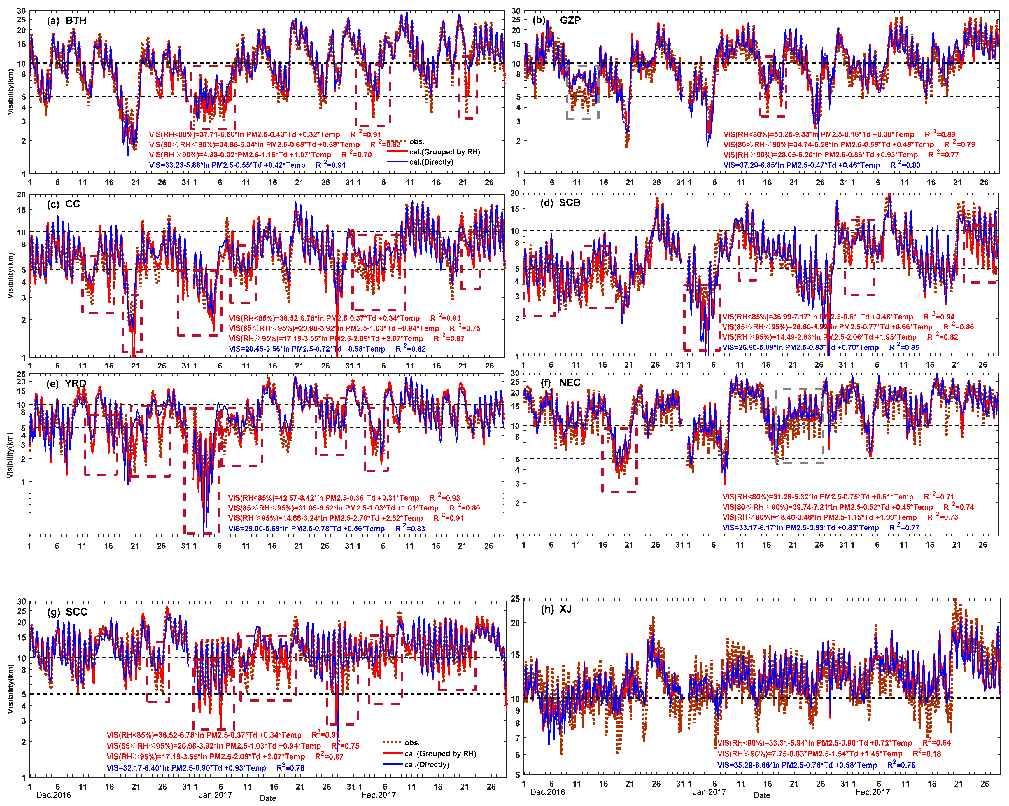
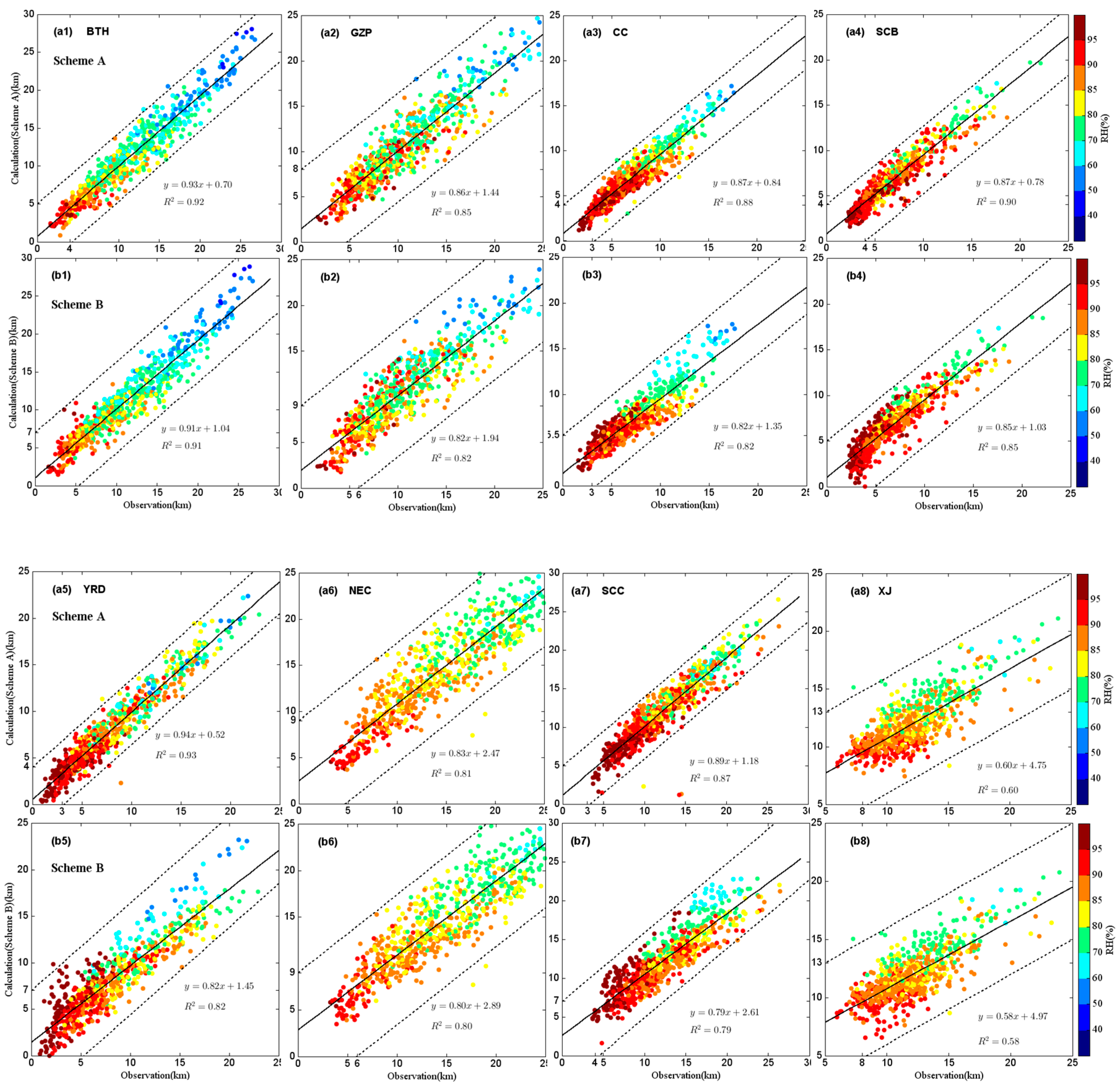
3.3. Multivariate Nonlinear Regression Equations of Visibility with PM2.5 Concentrations and Humidity
Under different RH levels, the fitting relationships between visibility and PM
2.5 concentrations are significantly distinct. Therefore, using the same RH grouping methods as in
Section 3.2, the multiple nonlinear regression equations of visibility, PM
2.5 concentration, and ambient humidity (represented by T and T
d) of the eight regions are established respectively and this method is defined as Scheme A. As the comparisons, according to the previous regression methods (the datasets are not grouped by setting RH levels), we directly established the multivariate nonlinear regressions of visibility and the same factors (Scheme B). The fitted visibility calculated by the two schemes is recorded as CAL
a and CAL
b, respectively.
Figure 4 shows the calculated visibility from the two schemes and the actual observations. It is clear that CAL
a of the eight regions (except XJ) are closer to the actual observations compared with CAL
b. Especially, Scheme A has greatly improved the calculation capability of low visibility. For example, a continuous low visibility event was observed in BTH from January 1 to 9, 2017 and the minimum visibility was only 2.9 km (orange box in
Figure 4a). Compared with observed visibility, the mean bias of CAL
a is 0.8 km while that of CAL
b is 2.3 km. A low visibility event with the minimum value of 2.5 km occurred in SCB from December 12 to 18, 2016 (orange box in
Figure 4d). The mean bias of CAL
a during this event is 1.2 km while that of CAL
b is 3.3 km. However, both the error of CAL
a and CAL
b in XJ is much larger than that in other regions. The R
2 of Scheme A and B in XJ is only 0.18–0.64 and 0.75 (
Figure 4h), while those in other regions are 0.70–0.93 and 0.77–0.91, respectively. The insufficient number of samples may be the major reason for the poorest visibility fitting in Xinjiang (
Table 1).
Figure 5 compares the calculated visibility with the observed visibility under different RH conditions. It is obvious that compared with CAL
b, CAL
a under all RH levels is closer to the observations. Especially under high humidity (RH > 90%) conditions, the calculation accuracy of CAL
a is clearly higher than that of CAL
b. According to the coefficient of determination (R
2), both CAL
a and CAL
b of NEC, GZP, and XJ have worse fitting precision compared with other regions, which may be related to sample sizes, density of meteorology sites, and PM
2.5 sites (
Table 1).
In order to further compare the low visibility fitting accuracy of the two schemes, the statistics of calculations under visibility < 5 and 3 km are given in
Table 2. It can be seen that the advantage of CAL
a for 5 and 3 km calculation is clearly more significant than CAL
b. CAL
a only slightly overestimates the low visibility of China (except SCC). For the five low visibility regions (BTH, GZP, CC, SCB, and YRD), the MB and MAE values under visibility < 5 km are 0.16–0.40 and 0.61–1.06 km, 27–62% and 18–46% lower than those of CAL
b, respectively. The MBs and MAEs of CAL
a under visibility < 3 km are −0.03–0.26 and 0.44–0.78 km, 26–93% and 22–52% lower than those of CAL
b, respectively. RMSEs of CAL
a in the five regions under visibility <5 and 3 km are 0.77–1.01 and 0.48–0.95 km, 16–43% and 24–57% lower than those of CAL
b, respectively. It suggests that the low visibility (<5 and 3 km) forecast accuracy of Scheme A has been improved by 16–57%.
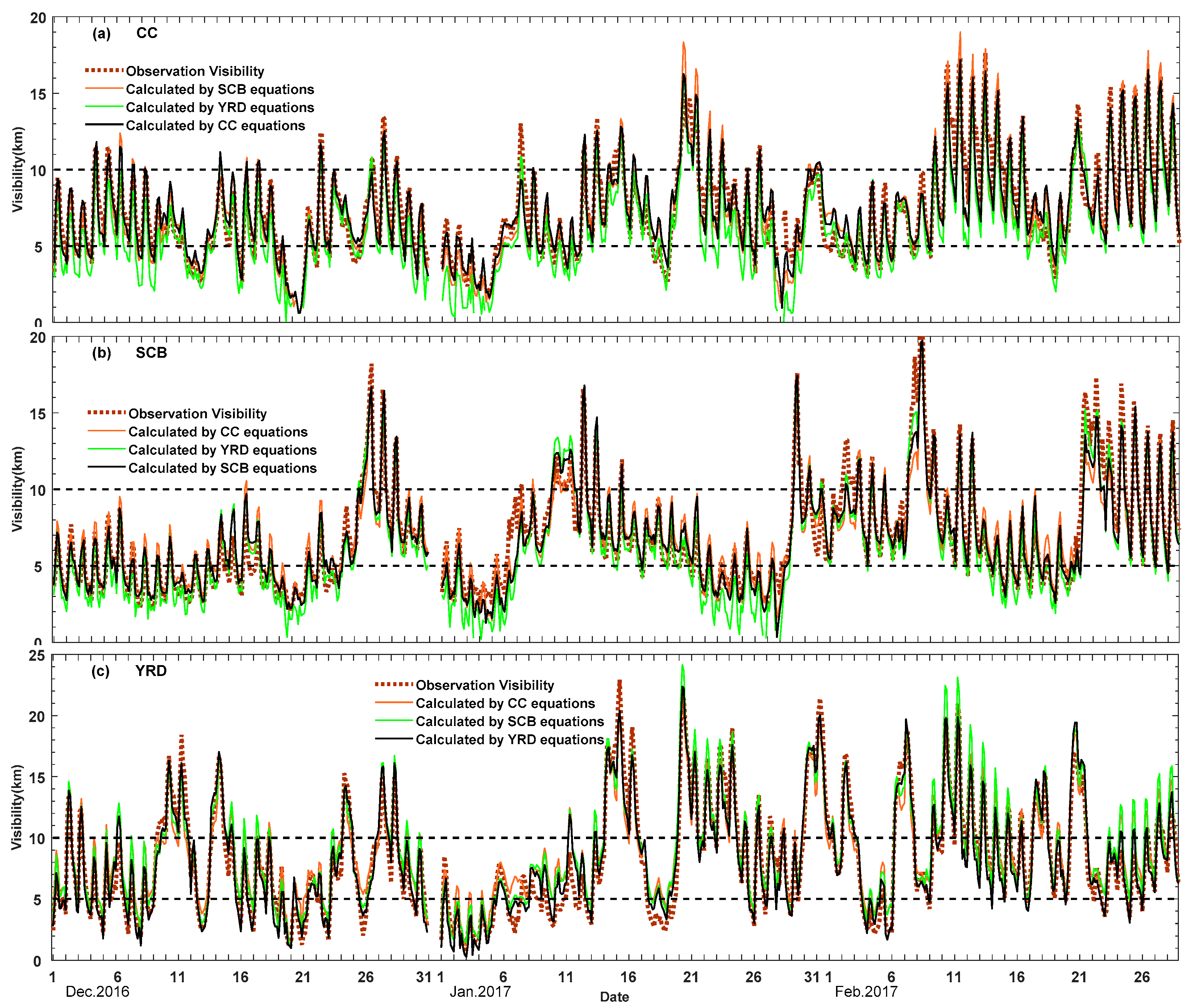
The datasets of CC, SCB, and YRD use the same RH grouping method in Scheme A. Moreover, the fitting relationships between the visibility, PM
2.5 concentration, and humidity of the three regions are relatively similar. At a constant RH level, the PM
2.5 concentrations that correspond to the visibility of 10 and 5 km are very close. Therefore, to test whether all the three equations can calculate the visibility in CC, SCB, and YRD well, the visibility is calculated by different equations of Scheme A respectively (
Figure 6). It is clear that all three equations can well estimate the visibility >5 km in CC, SCB, and YRD. However, the fitting accuracy of different equations under lower visibility conditions is obviously different. For instance, fitting visibility of YRD calculated by CC and SCB’s equations is far lower than the actual observations. Similarly,
Figure S1 (Supplementary Materials) shows the fitting visibility of BTH and GZP calculated by BTH and GZP’s equations respectively. As can be seen, BTH’s equations overestimate the low visibility in GZP, and GZP’s equations slightly underestimate the low visibility in BTH. Thus, it is reasonable to calculate the calculated visibility of the eight regions with respective visibility multivariate nonlinear equations. It also shows that the regional division in this paper is reliable to a certain extent.
3.4. Reasons Analysis on Poor Fitting Accuracy in NEC, GZP and XJ
Section 3.4 shows that CAL
a of NEC, GZP, and XJ have worse fitting precision compared with other regions. As can be seen in
Figure 1 and
Table 1, both PM
2.5 and meteorology sites in NEC, GZP, and XJ are far less than those of other regions. For example, the number of PM
2.5 sites in GZP and XJ are only 45 and 33 respectively. Accordingly, the total samples used to establish the visibility fitting equations are also the least. The insufficient samples are probably one of the main reasons for the poor fitting accuracy of calculated visibility in the three regions.
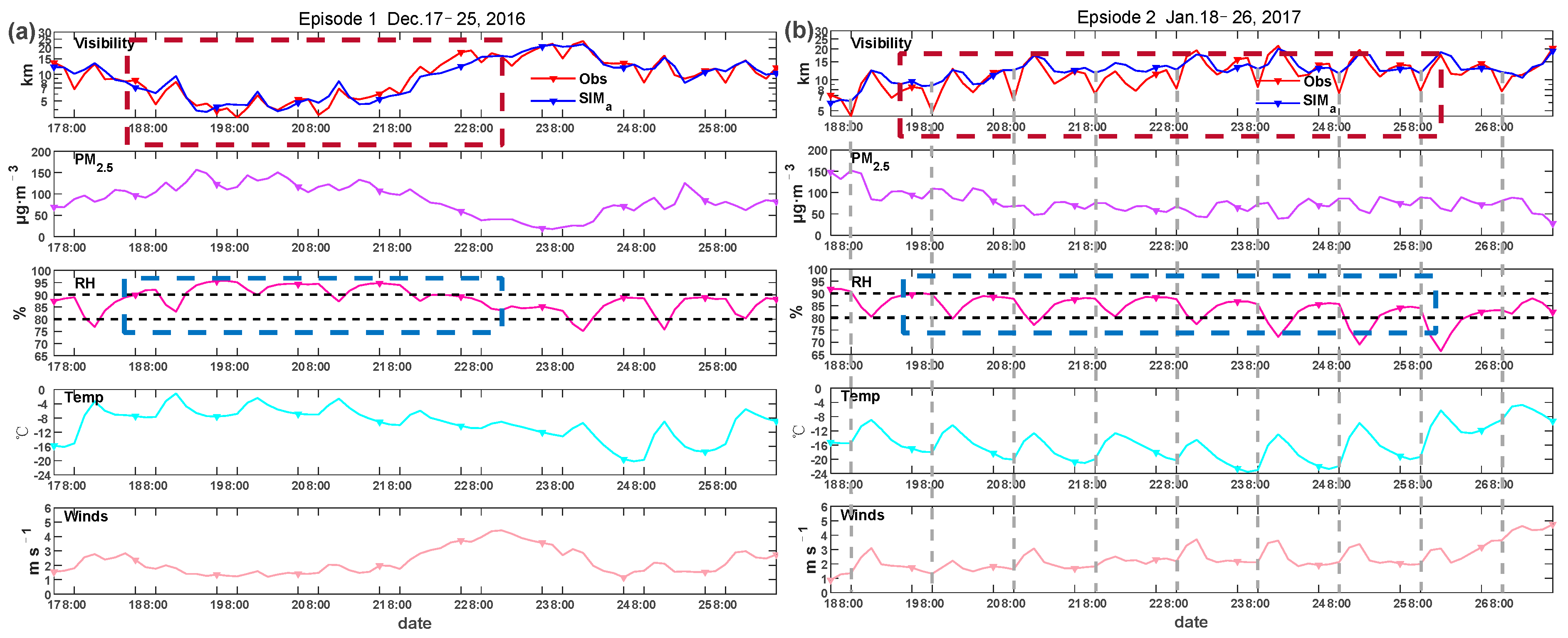
As can be seen in
Figure 4f, Scheme A well predicts the low visibility event in NEC during 17–25 December 2016 (Episode 1), but does not well predict the low visibility during 18–26 January 2017 (Episode 2).
Figure 7 shows the observed visibility, CAL
a, PM
2.5 concentrations, and surface meteorological factors in NEC during the two episodes. It can be noted that observed visibility at 08:00 (LT) in Episode 2 is much lower than that at other times. Compared with Episode 1, low visibility at 08:00 in Episode 2 is seriously overestimated. According to the present weather phenomenon, regional fogs were observed at 08:00 (LT) every day of Episode 2. However, the calculated RH values at 08:00 during Episode 2 are lower than 90%, with a maximum of 89.2% and a minimum of 83.1%. It can be seen that there are probably some errors and uncertainties of the RH calculation in NEC, which may be due to the insufficient samples caused by the lack of meteorology stations. As can be seen in
Figure 1, the NEC covers an area of about 450,000 km
2, with 88 meteorology sites distributed. But its density is only 1.95 per 10,000 km
2. By comparison, the density of meteorology sites in BTH and YRD is 7.10 and 6.56 per 10,000 km
2, respectively, far higher than that in NEC. Therefore, the insufficient samples of meteorology may be one of the major reasons for the mismatch between the fog phenomenon and the calculated RH at Episode 2.
3.5. Test of Visibility Forecast Ability of Scheme A
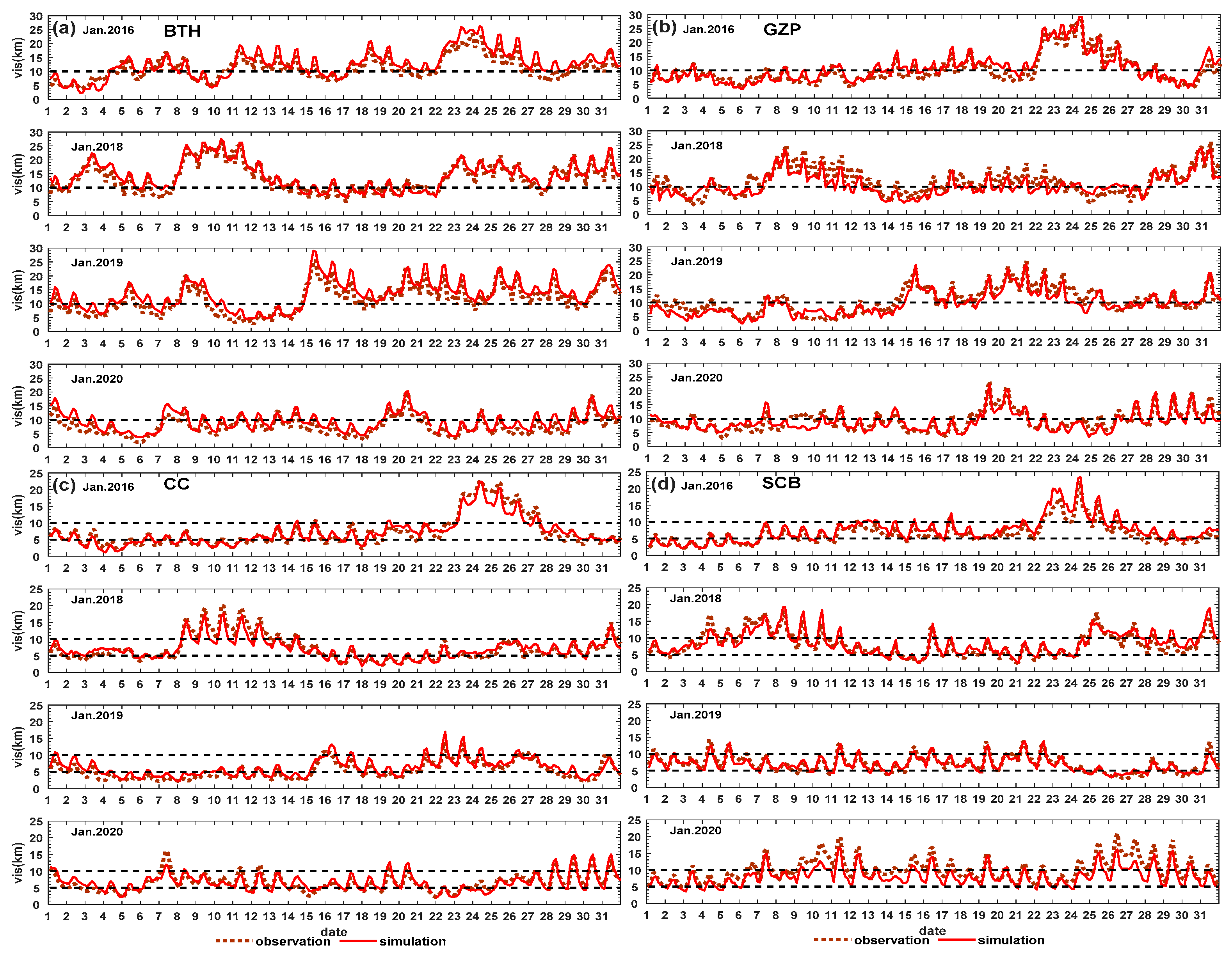
To examine the applicability of Scheme A, the visibility of the eight regions in January of 2016–2020 (except 2017) is calculated by Scheme A, and the results are compared with the actual observation (
Figure 8 and
Figure S2). The statistics of the calculations under visibility <5 km are shown in
Table 3 and
Table S1.
In general, the calculated and observed visibility of BTH, GZP, CC, SCB, YRD, and SCC have similar trends. Numerically, Scheme A slightly overestimates the visibility from 2016 to 2020. The correlation coefficient between the observed and fitted visibility is 0.88–0.96, which all pass the significance t-test at the 0.01 level. Especially, MAE, MB, and RMSE under low visibility (<5 km) conditions are 0.44–1.41, −1.33–1.24, and 0.58–2.36 km, respectively. It suggests that Scheme A can well predict the low visibility in middle and eastern China. The correlation coefficient between the observed and calculated visibility of NEC and XJ is only 0.59–0.85, far lower than that in other regions. The worse visibility forecast ability in NEC and XJ may be due to the poorer fitting accuracy of their visibility fitting equations.
We also compare the fitting visibility calculated by Scheme A with the results of previous visibility (extinction coefficient) regression parameterization schemes. Zhou et al. (2016) established a multiple regression equation of visibility in YRD, and the R2 was 0.816. This equation predicted the visibility in the winter of 2014–2015 well, with the correlation coefficient of 0.77. Fan et al. (2016) established multiple regression equations of visibility, PM2.5 concentration, and RH in Hangzhou, Ningbo, and Wenzhou. Jiang et al. (2018) compared the fitting visibility in Lin’an calculated by different visibility regression equations (Lin et al., 2009; Chen 2013; Shen, 2016). The four cities are all located in YRD. The R2 of these equations was 0.32–0.88, and the calculation accuracy under low visibility conditions was relatively low. As comparisons, the R2 values of the visibility regression equations for YRD in this study are 0.80–0.91 and the correlation coefficients between observations and calculations from 2016–2020 are 0.90–0.96, all higher than those of previous regression methods. Besides, Scheme A greatly improves the prediction ability of low visibility forecast in YRD, with the RMSEs under visibility <5 km of 0.88–1.03 km. Chen et al., 2012 established the regression equations of extinction coefficient, RH, aerosol volume concentration, and coarse to fine volume ratio in the North China Plain. The R2 was 0.89–0.92 while that of Scheme A is 0.92. Overall, compared with previous regression methods, Scheme A in this study can well predict the variations in winter visibility in China. Especially, Scheme A is confirmed to be reliable and applicable for the low visibility prediction (<5 km). This study provides a new visibility parameterization for the haze–fog numerical prediction system.
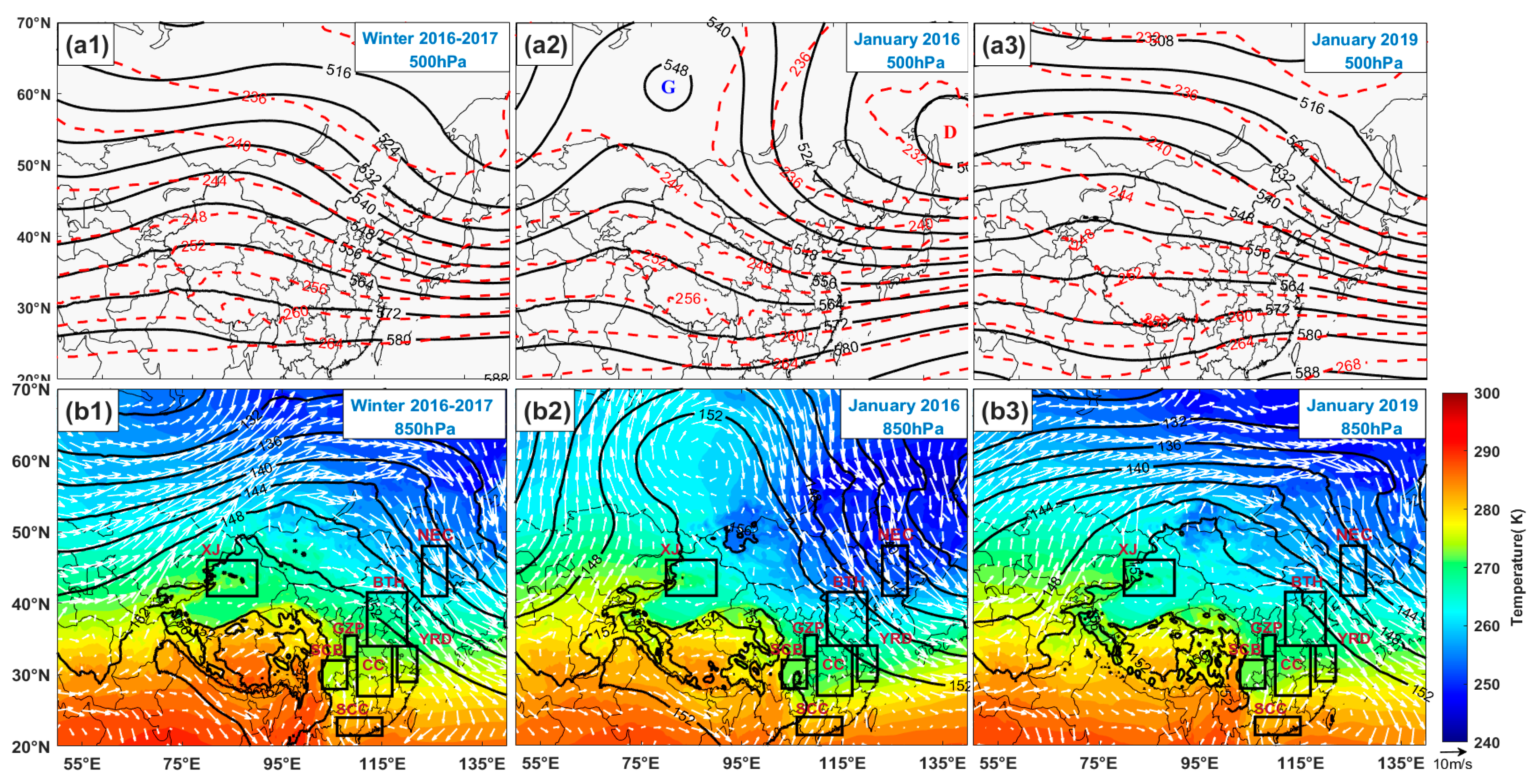
Comparing the visibility forecast accuracy between different years, it is clear that the calculated visibility of BTH, NEC, and XJ in 2019 and 2020 had higher fitness than that in 2016 and 2018, while the calculated visibility in CC, SCB, YRD, and SCC from 2016 to 2020 all had good fitting degrees. Previous studies have shown that the upper air circulation patterns affecting northern and central China in the winter of 2016 and 2018 were obviously different from those in 2017 and 2019 (Liu et al., 2019). To investigate whether the differences in upper air circulation patterns result in the poorer fitting degrees of visibility in BTH, GZP, and NEC in 2016 and 2018,
Figure 9 shows the average circulation situations at heights of 500 and 850 hPa during the winter of 2016–2017, January 2016 and January 2019 (weather situations in January 2018 and January 2020 are similar to those in 2016 and 2019 respectively, so they are not shown here).
As it can be seen, during the winter of 2016–2017, the synoptic situations at heights of 500 and 850 hPa are dominated by the distinct zonal circulation, suggesting weak winds and stable atmospheric conditions in BTH, GZP, and NEC. The upper-level circulation situations in 2019 and 2020 are basically similar to those in the winter of 2016–2017. Accordingly, the calculated visibility in 2019 and 2020 calculated by Scheme A, which is based on data of winter 2016–2017, have good fitting degrees. However, there are large changes in synoptic situations in 2016 and 2018. The circulation patterns in the mid-troposphere in the two years are dominated by distinct meridional circulation, suggesting strong cold air activity and high wind speeds (
Figure 9b) affecting northern and middle China. Correspondingly, the visibility in BTH, GZP, and NEC has not been well predicted in the two years. The strong meridional circulation has relatively smaller influences on the southern and eastern regions such as CC, SCB, YRD, and SCC. Thus the fitting degree of visibility in the four regions in 2016 and 2018 have no significant difference compared with that in 2019 and 2020. The results show that Scheme A performs better under similar circulation situations with the winter of 2016–2017. And this may be the main reason for the better visibility fitting degree in BTH, GZP, and NEC in 2019 and 2020.
4. Conclusions
With rapid urbanization and increasing pollutant emission, low visibility has become a pervasive and urgent environmental problem in China and its prediction accuracy is therefore important, especially for low visibility conditions. However, current visibility parameterizations tend to overestimate the low visibility during haze–fog events. The key point of low visibility calculation and prediction depends on a reasonable understanding of the correlation between visibility, PM2.5 concentration, and relative humidity (RH). Using the winter observations of PM2.5 concentration and meteorology from 2016 to 2017, under different RH levels, the relative contribution differences of changes in PM2.5 concentration and humidity to visibility decrease in the eight regions of China as well as their regional differences are discussed. Based on these contribution differences, new visibility multivariate nonlinear equations applicable to eight regions of China are established and evaluated.
Low visibility in winter always occurs during periods with severe PM2.5 air pollution and high humidity. Because of the regional distribution differences of PM2.5 concentration and RH, their contribution to visibility reduction also has obvious regional differences. Under different RH levels, the fitting relationships of visibility with PM2.5 concentration and RH are also distinct. Considering these differences, the data groups of BTH, GZP, and NEC are divided into 3 groups: RH < 80 %, 80 ≤ RH < 90 % and RH ≥ 90 %, data groups of CC, SCB, SCC, and YRD are divided into RH < 85%, 85 ≤ RH < 95 % and RH ≥ 95 %, and data groups of XJ are divided into RH < 90% and RH ≥ 90 %, respectively, and the relative contribution differences of PM2.5 concentration and RH changes to visibility decrease are investigated.
Under relatively low RH conditions (<80% or 85%), the visibility in China (except XJ) is usually >10 km (NEC and SCC) or 5 km (BTH, GZP, CC, SCB, and YRD) and the PM2.5 concentration dominates the visibility changes within this range. As the RH increases, the PM2.5 concentration that corresponds to the visibility of 10 and 5 km gradually decreases, suggesting that the contribution of PM2.5 concentration to visibility reduction gradually decreases, while the contribution of RH becomes increasingly important. When the water vapor in the air reaches the saturation state (RH > 95%), the visibility degradation is mainly caused by the direct extinction of fog droplets, a very low PM2.5 concentration could lead to visibility <5 km. The PM2.5 concentration corresponding to the visibility of 5 km in CC, SCB, and YRD is approximately 30, 50, and 50 μg m−3 respectively, while that in BTH and GZP is 125 μg m−3. Moreover, at a constant RH level, the PM2.5 concentration that corresponds to the visibility of 10 and 5 km in BTH and GZP is always higher than that in other regions, indicating a higher contribution of PM2.5 to visibility variations in the two regions.
Based on these contribution differences, using the same RH grouping methods, the multiple nonlinear regression equations of visibility, PM2.5 concentration, T, and Td of the eight regions are established respectively (Scheme A). According to the previous regression methods, the multiple regression equations of visibility and the same factors are established directly as the comparisons (Scheme B). The calculated visibility from the two schemes is recorded as CALa and CALb. The statistical results show that CALa of the eight regions (except XJ) is closer to the actual observations. Especially, the advantage of Scheme A for 5 and 3 km evaluation under high humidity conditions is more significant compared with CALb. For the five low visibility regions (BTH, GZP, CC, SCB, and YRD), MAEs of CALa under visibility <5 and 3 km are 0.61–1.06 and 0.44–0.78 km, 18–46% and 21–52% lower than that of CALb, respectively. RMSEs of CALa under visibility <5 and 3 km are 0.77–1.01 and 0.48–0.95 km, 16–43% and 24–57% lower than those of CALb respectively, suggesting that the low visibility forecast accuracy of Scheme A is improved by 16–57%. Moreover, Scheme A can well predict the variations in winter visibility in BTH, GZP, CC, SCB, YRD, and SCC from 2016 to 2020. The correlation coefficient between the observed and fitted visibility is 0.88–0.96, which all pass the significance t-test at the 0.01 level. The MAEs, MBs, and RMSEs under low visibility (<5 km) conditions are 0.44–1.41, −1.33–1.24, and 0.58–2.36 km, respectively. Overall, Scheme A is confirmed to be reliable and applicable for the visibility prediction in many regions of China (except XJ).
This study provides a new visibility parameterization algorithm for the haze–fog numerical prediction system. The physical meaning of this algorithm is relatively clear, and it is proven to be applicable to many areas of China, with simple calculations, high time resolution, and relatively high forecast accuracy of low visibility. However, this method has some limitations and uncertainties. This method has been proved to be suitable for winter, but in spring, summer, and autumn, some weather phenomena such as dust and precipitation could also lead to the occurrence of low visibility, so it may be not applicable to those three seasons. Moreover, its visibility forecasting effect is greatly affected by the number of samples of the study region. The uncertainty of RH calculation could also affect the accuracy of visibility multiple regressions. These limitations deserve to be further studied.


