Article

Emissions of H2S from Hog Finisher Farm Anaerobic Manure Treatment Lagoons: Physical, Chemical and Biological Influence

Department of Agronomy, Purdue University, 915 W. State St., West Lafayette, IN 47907, USA
*
Author to whom correspondence should be addressed.
Atmosphere 2022, 13(2), 153; https://doi.org/10.3390/atmos13020153
Submission received: 14 December 2021 / Revised: 11 January 2022 / Accepted: 12 January 2022 / Published: 18 January 2022
(This article belongs to the Special Issue Feature Papers in Atmosphere Science)

Abstract

:
Hydrogen sulfide (H2S) from hog operations contributes to noxious odors in the surrounding environment and can be life-threatening. There is, however, limited understanding of what influences H2S emissions from these farms. Emissions of H2S were measured periodically over the course of two years at hog finisher farms in humid mesothermal (North Carolina, NC, USA) and semi-arid (Oklahoma, OK, USA) climates. Emissions were determined using an inverse dispersion backward Lagrangian stochastic model in conjunction with line-sampled H2S concentrations and measured turbulence. Daily emissions at the two lagoons were characterized by low emissions on most days with occasional days of high emissions. Mean annual area-specific emissions were much lower for the NC lagoon (1.32 µg H2S m−2 s−1 ± 0.07 µg H2S m−2 s−1) than the OK lagoon (6.88 µg H2S m−2 s−1 ± 0.13 µg H2S m−2 s−1). Mean annual hog-specific emissions for the NC lagoon were 0.75 g H2S hd−1 d−1 while those for the OK lagoon were 1.92 g H2S hd−1 d−1. Emissions tended to be higher during the afternoon, likely due to higher mean winds. Daily H2S emissions from both lagoons were greatest during the first half of the year and decreased as the year progressed and a reddish color (indicating high populations of purple sulfur bacteria (PSB)) appeared in the lagoon. The generally low emissions at the NC lagoon and higher emissions at the OK lagoon were likely a result of the influence of wind on mixing the lagoon and not the presence of PSB.

1. Introduction

Hydrogen sulfide (H2S) is a major source of odor and an asphyxiant. Consequently, emissions of H2S are monitored nationally through the Comprehensive Environmental Response, Compensation and Liability Act (CERCLA) and the Emergency Planning and Community Right-to-Know Act (EPCRA). This study is part of the National Air Emissions Monitoring Study (NAEMS) [1]. Hydrogen sulfide is formed from animal manure sulfur compounds including primarily inorganic sulfate and organic sulfur compounds [2]. Sulfate-reducing bacteria near the bottom of the lagoon produced HS- from the settled manure [3]. The soluble HS- equilibrates with H2S as a function of pH. The H2S is only slightly soluble in water and consequently exists both in the lagoon solution and in micro-bubbles as the partial pressure of H2S increases with increased depth [4]. The H2S is transported from lower layers of the lagoon to the liquid–atmosphere interface by diffusion and ebullition.
Many anaerobic treatment lagoons have periods in which they appear reddish-purple [5]. This coloring is usually a result of the presence of large populations of purple sulfur bacteria (PSB) from the family Chromatiaceae in the phototrophic regions of the lagoon. These bacteria can photosynthesize anoxygenically and oxidize H2S rising from the lower reaches of the lagoon to SO42− [5,6], consequently reducing emissions from the lagoon surface [7,8]. The optimal pH for PSB ranges from 7.5 to 8.2 [7]. Purple non-sulfur bacteria (PNSB) have also been found in swine lagoons but are unable to oxidize zero-valent sulfur to sulfate and hence have a competitive disadvantage in a HS--rich anaerobic lagoon [5].
Prior studies reporting hydrogen sulfide emissions from anaerobic swine waste lagoons show highly variable emissions. A study that used a micrometeorological approach to calculate the emissions from a swine finishing operation in Missouri reported a mean H2S emission rate of 1.57 g H2S hd−1 d−1 from 14 days of measurements in late summer and early fall [9]. A portable wind tunnel was used to calculate H2S emissions of between 1.70 and 2.73 g H2S hd−1 d−1 from 12 days of measurements in late spring to early summer from three lagoons in Minnesota [10]. A dynamic chamber was used to calculate emissions from hog operations in NC, ranging from negligible amounts during the winter to 0.019 g H2S hd−1 d−1 during the summer in an 84-day study [11].
This analysis of the annual and diurnal variations in hydrogen sulfide emissions from finisher operations in differing climates used measurements made during the National Air Emissions Monitoring Study (NAEMS).

2. Experiments

Measurements of hydrogen sulfide emissions were made over the course of two years (2008, 2009) at waste lagoons on hog finisher farms in humid mesothermal (NC, USA) and semi-arid (OK, USA) climates.

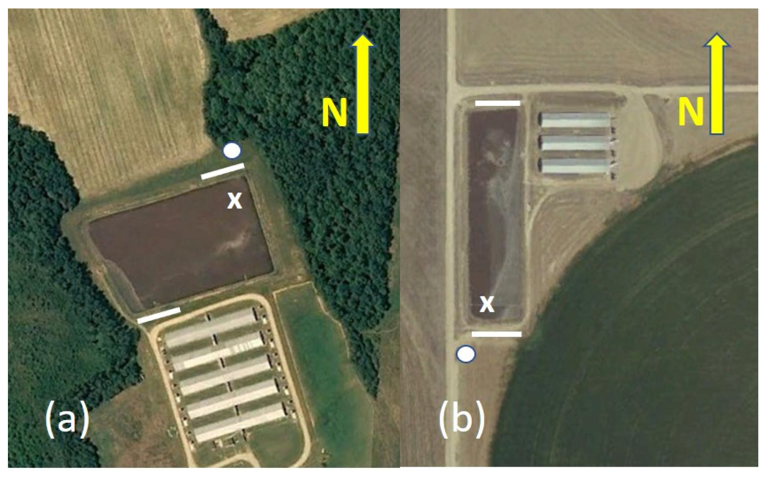
2.1. Farm Descriptions and Operations

The North Carolina finisher facility consisted of five barns, an office and a waste lagoon (Figure 1a). The facility had a capacity of 8000 finishing pigs in five units [12]. Construction of the farm was completed in 1996. Manure from the barns was transferred daily to the lagoon by pull plug and lagoon water recharge. Wastewater combined into one inlet. The rectangular waste lagoon was located to the north and was separated by a drainage swale from the barns. The lagoon area was 18,987 m2 and volume was 45,973 m3. Maximum liquid depth was 3.3 m. Wastewater was removed for irrigation as weather permitted. Sludge from the lagoon had not been removed since construction (15-year sludge removal cycle) and was approximately 0.3 m thick. Producer-reported activity is provided in Table 1.
The Oklahoma finisher facility consisted of three barns and a waste lagoon (Figure 1b). The facility had a maximum capacity of 3024 finishing pigs [13]. Construction was completed in 1997. Manure from the barns was transferred three times a week to the lagoon by a pull plug system with lagoon water recharge. Wastewater from all three units combined into one inlet emptying into the rectangular lagoon west of the barns. At maximum capacity, the lagoon had a liquid depth of 6 m, a surface area of 22,500 m2 and a volume of 28,700 m3. Liquid was removed approximately every six months. Sludge from the lagoon had not been removed since construction (20-year sludge removal cycle) and was approximately 0.3 m thick. Producer-reported animal inventories and activity were provided in Table 1.
Finisher hog operations typically grow hogs in batches with short periods of time between batches in which no animals are present in a barn. Measurements were made both when hogs were housed in the barn and when the barns were emptied and cleaned. Comparing emissions from the lagoons when the barns contained hogs with those when the barns were empty provided a measure of the proportion of H2S emissions that were due to fresh manure being added to the lagoon. Since the gaseous lagoon emissions emanate from manure and effluent residing in the lagoon for multiple months, it was assumed that the number of animals contributing to the lagoon was the maximum capacity of the farm. The producer-reported and study-observed lagoon characteristics for the two farms are indicated in Table 2.

2.2. Measurements

Hydrogen sulfide emissions from the waste lagoons were measured at the two finisher operations to determine the variation in emissions with time of year, meteorological conditions and facility operation. Emissions were measured using H2S concentration and wind turbulence measurements in a backward Lagrangian stochastic model. Measurements were made for approximately two-week periods at each facility for each quarter over two years. Measurements were made for 105 days at the NC lagoon and 148 days at the OK lagoon. Calibration verification checks of the instruments on-site were conducted at the beginning and end of each measurement period when field staff were on-site.
Concentrations of H2S around each lagoon were measured by pulsed-fluorescence (Model 450i, Thermo Fisher Scientific, Waltham, MA, USA) from air drawn at approximately 7 lpm from synthetic open-path systems (S-OPS) on the north and south sides of the lagoon (Figure 1). Each of the S-OPS provided a single flow of air mixed uniformly from ten flow-balanced inlets with 1 µm Teflon® filters spaced evenly along a 50 m long 9.5 mm Teflon® line at 1 m above berm level (abl). The two S-OPS were sampled by a gas sampling system (GSS) based on similar sampling systems for animal housing [13]. Air was drawn from each of the S-OPS sequentially for 15 min by the GSS, with only the last 2 min of concentration measurements used for analyses. Stationarity of the source emission over the half-hour interval was assumed. Stationarity of the flow was assumed when the wind direction standard deviation was less than 30°. A valid upwind S-OPS air sample was defined as having a half-hour mean wind direction less than 60° off the S-OPS perpendicular with the lagoon downwind and wind direction standard deviation of less than 30°. A valid downwind S-OPS air sample was defined as having a half-hour mean wind direction less than 60° off the S-OPS perpendicular with the lagoon upwind and wind direction standard deviation of less than 30°.
The performance of the SO2/H2S analyzer was checked with continuous emissions monitoring (CEM) zero air and a standard gas at span concentration (1420 µg m−3) with response required to be within 10% accuracy. The errors associated with the calibration gas and the diluter were 3% and 1% respectively. The SO2/H2S analyzer minimum detection limit (MDL) (3σ) was 3 µg m−3 (NC) and 4 µg m−3 (OK) [12]. The mean zero bias concentration was +0.4 µg m−3 (NC) and +2 µg m−3 (OK) [12]. Multipoint calibrations of the SO2/H2S analyzer were conducted eight (OK) and seven (NC) times [12]. Instrument response was converted into measured concentrations by multiplying the response by the long-term mean ratio of diluted calibration gas to instrument reading derived from the calibration verification checks. The performances of the S-OPS and GSS were assured by flow and pressure measurement checks of the balance of inlet flows and integrity of sample tubing.
Sensors for the meteorological measurement of barometric pressure (Model 278, Setra, Boxborough, MA, USA), air temperature and relative humidity (Model HMP45C, Vaisala Oyj, Helsinki, Finland), as well as solar radiation (Model 210, LiCOR, Lincoln, NE, USA), were located on a mast situated on the berm near a corner of each lagoon (Figure 1). Measurements were recorded every 5 min and averaged to half-hour intervals. The wind direction and wind speed measurements used in defining valid measurement periods and turbulence statistics used by the emissions model were measured using a 3D sonic anemometer (Model 81000, R.M. Young, Traverse City, MI, USA) located on the meteorological mast at 2.5 m abl. Measurements were recorded at 16 Hz and averaged to half-hour intervals. Sonic anemometer measurements were quality assured by sensor inter-comparisons and zero flow checks. To be considered a valid 5 min period of measurements, at least 90% of the possible 16 Hz values had to be present.
Turbulence statistics used in the emissions model were considered representative of the 30 min statistic interval if at least 50% of the possible 5 min intervals had valid measurements. Validity of the calculated turbulence statistics for each half-hour interval were also evaluated based on upwind fetch conditions. Fetch to the barns whose exhaust contributed to the H2S concentrations were of particular concern. The barns 20 m to the south of the NC lagoon berm had a fetch ratio 3:10 (Figure 1a). Fetch to forest to the east and west were both 3:10. All measurements when the wind was from 135° through 225° were excluded from analysis. Barns to the west of the OK lagoon berm had a fetch ratio of 6:10 to the east side of the lagoon (Figure 1b). Fetch in all other directions was better than 1:100, with upwind interference from center-pivot irrigated crops. Due to the proximity of the barns, emissions from wind directions of 90° to 135° were excluded from analysis.
The state of the lagoon at 0.3 m depth was monitored during non-freezing conditions using an instrumented float located approximately 5 m from the lagoon shore near the meteorological mast and away from the lagoon waste inlets (Figure 1). Measurements included liquid temperature (Model 107-L, Campbell Scientific, Logan, UT, USA), pH (Model CSIM11, Campbell Scientific, Logan, UT, USA), and the oxidation reduction potential (ORP) referenced to a platinum electrode (Model CSIM11, Campbell Scientific, Logan, UT, USA). Measurements were made every 5 min and averaged to half-hour intervals. There were 6415 and 5645 valid half-hour lagoon temperature values for the NC and OK lagoons respectively. The pH probe performance was evaluated using three standards (pH 4, 7 and 10) for response and a Quality Control Check sample solution [14] for stability, with the requirement that the sensor response be within 0.05 pH units, or 3 mV of the standards. There were 7931 and 5023 valid half-hour pH values for the NC and OK lagoons respectively. The ORP probes were evaluated for stability using Zobell’s KCl solution [15], with the requirement that the sensor be within 1 mV of the reference solution. There were 7585 and 5645 valid half-hour ORP values for the NC and OK lagoons respectively.
Producers provided commercially analyzed lagoon liquid composition measurements that were made prior to field applications in accordance with their individual USDA Natural Resource Conservation Service nutrient management plans in accordance with guidelines provide by the USEPA [16]. The sulfur content and pH of the liquid were analyzed ten times at the NC lagoon and three times at the OK lagoon. Although the steady-state fraction of both total S and organic S in a lagoon depends on the hog feed [17,18], the fraction of organic S was expected to be relatively small compared to H2S [2]. The maximum potential hydrogen sulfide concentration in the liquid samples was estimated from the sample S content and pH, assuming no organic S [11].
Although no measurements of PSB were made in this study, the potential for biological activity in the lagoon associated with PSB populations was assessed based on lagoon pH range [5], oxidation-reduction potential (ORP) range [5], color [5] and temperature range [5,19]. In addition, the appearance of the lagoon surface was recorded during site visits (Table 2). A reddish lagoon surface is associated with high PSB or PNSB populations [5]. Since PNSB have a competitive disadvantage in HS--rich environments [5], it was assumed that the dominant bacteria producing the reddish coloration were PSB. If the reddish color was observed during both the site visit at the beginning and that at the end of the measurement period, it was assumed that high PSB populations were present during the entire measurement period. On the other hand, if the reddish color was evident during only one of the two visits, the PSB population was assumed to be high only within one week of the observation.
Sludge depth estimates during the study were based on both producer-provided and on-site project measurements (Table 2). Project measurements were made infrequently using a ‘sludge gun’ (Markland Specialty Engineering, Ltd., Georgetown, ON, Canada). Average sludge depth for a given day was based on nine evenly distributed measurements. Information concerning farm operations were routinely collected from the producers.
Emissions of H2S, calculated over half-hour averaging periods, were determined by single value decomposition of the matrix composed of a flux versus concentration relationship for each of the S-OPS around the lagoon obtained using a backward Lagrangian stochastic (bLS) model (WindTrax; Thunder Beach Scientific, http://www.thunderbeachscientific.com, accessed on 19 December 2019), using the turbulence statistics derived from the on-site sonic anemometer measurements. The background concentration (Cbg) was determined in the solution to the concentration-flux matrix and not from a designated upwind concentration measurement since turbulence can contribute mass disproportionately to mean wind direction. Half-hour averaging periods were excluded from analysis when one or more of the following was true: (1) the absolute value of the Monin Obukov length (L) was less than 2 m [20,21], (2) the friction velocity was less than 0.15 m s−1 [21,22], (3) less than 5% of the backward trajectory parcels originated within the lagoon source area, (4) the wind direction standard deviation was greater than 30°, (5) the mean wind direction was greater than 60° off the S-OPS perpendicular, or (6) the calculated Cbg was greater than the instrument MDL. The bLS emission model has a theoretical random error of 22% [22] and tracer-estimated error of between 5% and 36% [23]. Assuming a 22% emissions model error, the combined error of the half-hour measurements and emissions estimates was 24%. Seasonal and annual emissions were based on all valid half-hour emissions in a given season.
Daily emissions were based on the number of mean half-hourly emissions in an average day that were needed to estimate daily emissions within 30% of the mean day when the lagoon did not appear reddish (indicating relatively low populations of PSB). This was determined by randomly sampling half-hourly emissions, averaging the sampled emissions and comparing the resulting mean emission to the mean daily emission including all measurements. Days with sufficient half-hourly measurements to represent the day with 30% or less error were termed ‘representative’ days. The error of the daily mean emissions was estimated by dividing the relative error of the daily measurement by the square root of the number of representative days included in that emission estimate. Seasonal and annual mean daily emission errors were estimated by dividing the relative error of the daily measurement by the square root of the number of half-hourly values divided by the number of half-hourly values needed to define a representative day.
Emissions reported on a head basis from the lagoons were scaled by the mean animal population of the facility and not the animal population at the time of measurements. The mean populations over the course of the study were 5602 hd and 2742 hd at the NC farm and the OK farm, respectively. An evaluation of this assumption was made based on relatively short-term intervals in which animals were not present in the barns of each farm (Table 1).
Wind shear at the lagoon surface promotes the emission of both dissolved H2S and H2S contained in bubbles lying under a surface film (through bursting). The wind speed, as a proxy for this process, was related to daily mean emissions using Grapher® 11.9 (Golden Software, LLC, Golden, CO, USA) according to the power law:
E i = α   ( U i ) β
where Ei was the daily H2S emission rate, α represented the lagoon source strength in the absence of wind and β represented the efficiency of turbulent mixing between the liquid and the boundary layer of the air overlying the lagoon.
Normalized daily mean emissions were defined as:
N i = [ Q i ( U i ) E l o w e r ( U i ) ] / [ E u p p e r ( U i ) E l o w e r ( U i ) ]
where power law functions (Equation (1)) were used to describe the upper (Eupper(U) and lower (Elower(U) bounds of the emissions relative to U, were defined using the calculated regression β from Equation (1) and visually adjusting α.
Comparisons between lagoon conditions with few measurements were evaluated using the nonparametric Wilcoxon rank sum test if not normally distributed [24]. Comparisons of lagoon conditions with more than 100 measurements were evaluated using the student’s t-test.

3. Results and Discussion

At the OK farm, the mean daily air temperature varied from −13 °C to 34 °C with the lagoon temperature reaching a high of 28 °C (freezing of the lagoon and damage to the probes at the OK lagoon prevented monitoring of lagoon temperatures during the winter so annual minimum temperatures were not measured). Wind speeds were high on the farm with a median wind speed of 4.0 m s−1. The OK lagoon depth varied from 5.3 m to 5.7 m. The mean daily air temperature at the NC farm varied from 1 °C to 28 °C with the lagoon temperature varying from 11 °C to 30 °C. The median wind speed was 1.1 m s−1. The NC lagoon depth varied from 1.5 m to 2.8 m and sludge depth varied from 0.8 to 0.3 m (Table 2).
Weather conditions and equipment failures influenced the number of valid emissions measurements at the farms. There were 1908 and 3861 half-hour emission measurements at the NC and OK farms respectively. Of these measurements, there were 1148 and 3176 valid half-hour emission measurements at the NC and OK farms respectively. The high loss of measurements at the NC lagoon compared to the OK lagoon was largely due to generally low wind speeds at the NC lagoon causing the friction velocity to be frequently below the 0.15 m s−1 threshold. Of the 144 days of measurements at the NC farm, there were 109 days with valid emissions measurements and 67 days with positive mean emission measurements. Of the 138 days of measurements at the OK farm, there were 107 days with valid emissions measurements and 84 days with positive mean emission measurements.

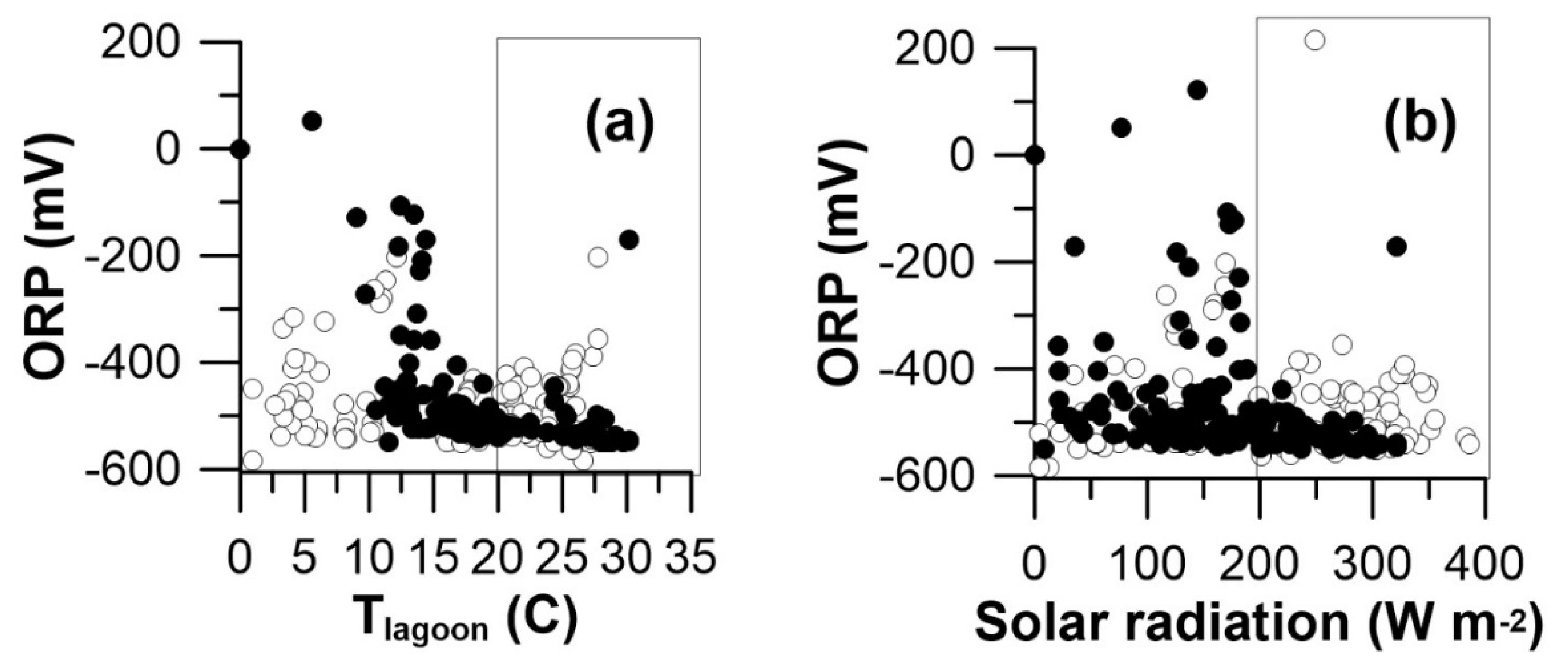
3.1. Lagoon Conditions

The lagoon temperature at 0.3 m depth was compared to the air temperature at 2.5 m height to assess the amount of thermal mixing in the upper 0.3 m of the lagoon. The average difference in daily mean lagoon and air temperatures was 3.7 °C at the NC lagoon and 2.0 °C at the OK lagoon. The relatively steady temperature environment and low wind speeds at the NC lagoon likely inhibited wind shear-driven overturning of the lagoon due to changes in lagoon thermal stability. Although the wider air temperature ranges at the OK lagoon and the freezing conditions during the winter could result in seasonal overturning of the lagoon as suggested for an IN dairy lagoon [25], the high wind speeds likely caused constant mixing in the lagoon, keeping the lagoon liquid temperature and air temperature closer at the OK lagoon than the NC lagoon.

3.2. Potential Biological Activity

The reddish surface appeared about mid-year in both lagoons (Table 2), indicating probable increased microbial populations in the lagoon. Lagoon pH, ORP, temperature and appearance (color) were evaluated to determine the likelihood of PSB in the anaerobic phototropic region of the lagoon. The daily mean pH ranges of the NC (7.3 to 8.0) and OK (7.4 to 8.2) lagoons were both within the optimal range for PSB growth (6.8 to 8.5) [5]. Both lagoons were strongly anaerobic most of the year: the mean daily ORP (0.3 m depth) for all measurement days varied from −171 mV to −550 mV at the NC farm and from −202 mV to −584 mV at the OK farm. Optimal lagoon temperatures for PSB populations corresponded with stronger reducing environments (negative ORP; Figure 2a). Higher solar radiation levels enhance the potential for PSB populations to grow yet were associated with the stronger reducing environmental conditions (Figure 2b). The least reducing environments (ORP least negative) were during the fall and winter. A reddish coloration of the lagoon surface, suggesting the presence of PSB populations, generally developed during the summer and fall (Table 2). The lack of reddish appearance of the lagoon until mid-summer (approximately DOY 180) suggested that PSB populations declined during the winter [18] and may have slowly rebuilt during the spring [5,7].
The reddish surface color of the lagoon was assumed the best indicator of significant PSB populations. Although the ORP was significantly different between the periods with or without the reddish surface color (Table 3), the differences were not considered physically significant. If the reddish color indicated large PSB populations, the presence of a reddish color to the lagoon should correspond with a decrease in ORP associated with the oxidation by the PSB. This was observed for the NC lagoon but not the OK lagoon (Table 3). Daily mean ORP did not show a distinct annual variation at either lagoon. Variation in ORP may have been driven instead by the mixing of the lagoon layer at 0.3 m depth with the surface (discussed below). Differences in lagoon temperature and pH in the presence or absence of a reddish surface were also statistically significant at both lagoons (Table 3). Although the pH of the lagoons was significantly different with difference in surface color, the mean pH with or without the reddish color were within the optimal pH range of 7.5 to 8.2 for PSB (Table 3).

3.3. Concentrations

The distribution of half-hourly H2S gaseous concentrations were strongly negatively skewed over both lagoons with the mean concentrations much higher than the median concentrations. The mean half-hourly concentrations were 9.4 µg H2S m−3 and 10.1 µg H2S m−3 for the NC and OK lagoons, respectively. The median half-hourly concentration measurements at 1 m abl on either side of the NC lagoon were 10.3 µg H2S m−3 and 8.5 µg H2S m−3, with the higher concentration nearer the barns. The median half-hourly concentration measurements at 1 m abl on either side of the OK lagoon were 2.5 µg H2S m−3 and 2.8 µg H2S m−3. The mean concentrations were similar to that reported for finishing hog manure storages in Minnesota [10]. The maximum half-hourly concentrations were 1073 µg H2S m−3 and 344 µg H2S m−3 at the NC and OK lagoons, respectively.
The lagoon liquid sulfur content was, on average, less for the OK lagoon than the NC lagoon, while the pH was higher for the OK lagoon than the NC lagoon (Table 4). The pH of the producer-reported OK lagoon analyses (Table 4) were higher than our measured values, while those for the NC lagoon were similar to our measured values (Table 3). Since the samples analyzed for field application (producer-reported analyses) were collected after several hours of mechanical agitation according to guidelines [26] while our measurements were made in situ at 0.3 m without mechanical agitation, differences in the pH at the OK lagoon may indicate lagoon nutrient stratification [26].
The sulfur content and pH of the NC lagoon were similar to the ‘Type 1 Feeder to finish lagoon’ [27]. The sulfur content of the OK lagoon was consistent with that of the ‘Type 1 Feeder to finish lagoon’ but the pH was much higher than the nominal 7.1 of the Type 1 lagoon [27].
Within the lagoon, the sulfur is typically present as HS, H2S, or SO42− [3,5,6]. Chemical analysis of lagoon liquid samples showed generally higher concentrations of sulfur (S) in the NC lagoon than the OK lagoon (Table 4). Purple sulfur bacteria oxidize the H2S to SO42−, which would not be emitted into the atmosphere and consequently would tend to maintain higher total sulfur concentrations in the lagoon [28]. The sulfur content of the NC lagoon liquid when the lagoon surface was reddish was not significantly different (p = 0.0125, 95% confidence interval of −0.0101 to 0.02; Mann–Whitney unpaired test) from that when the surface was not reddish. The sulfur content of the OK lagoon liquid could not be statistically evaluated due to the limited sample size. The lack of correlation between the reddish color (presumably indicative of PSB) and sulfur content might be expected if the emissions of S as H2S was not significantly reduced by the PSB activity converting the H2S or SO42, or if the reddish color was a result of large PNSB populations.

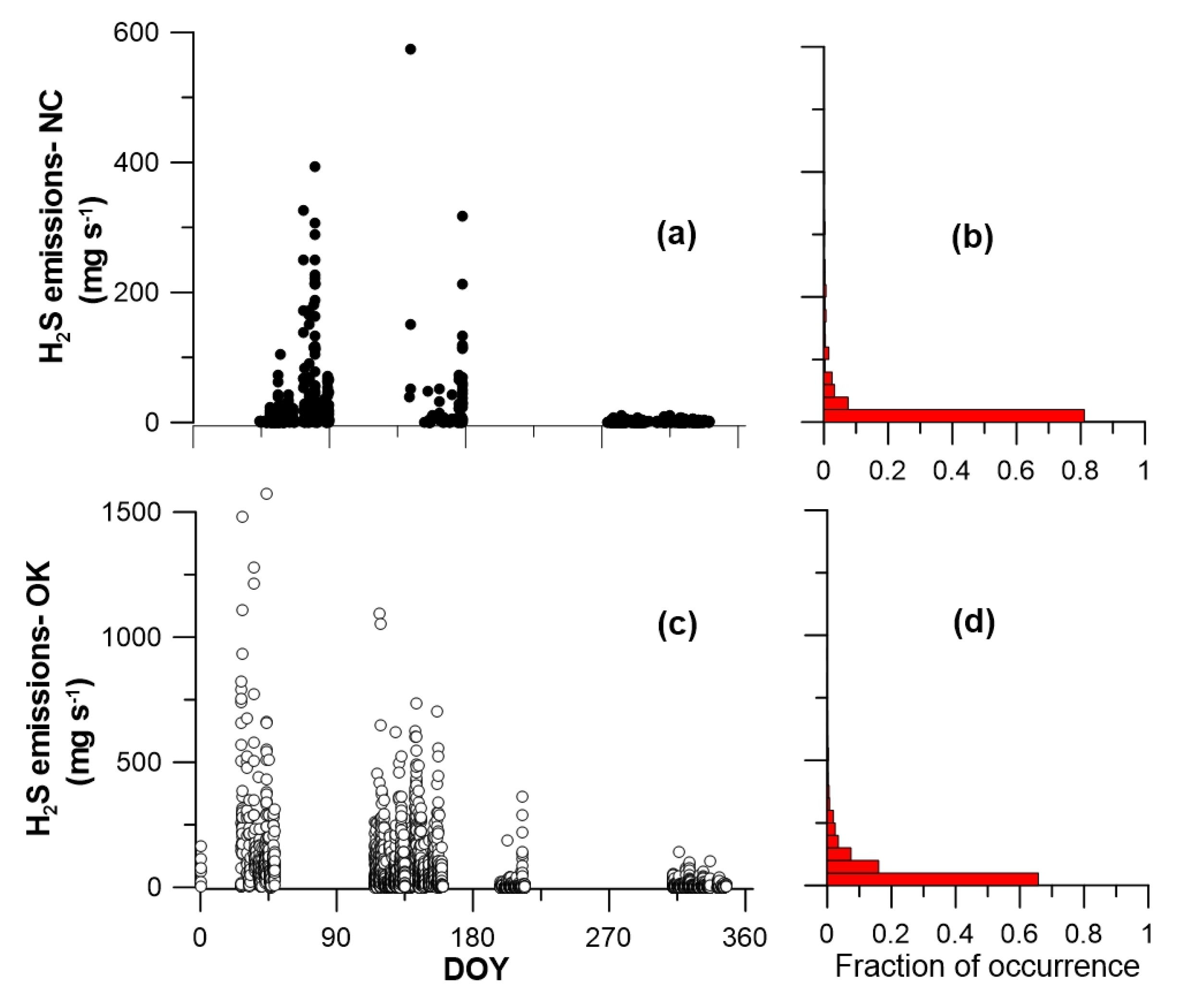
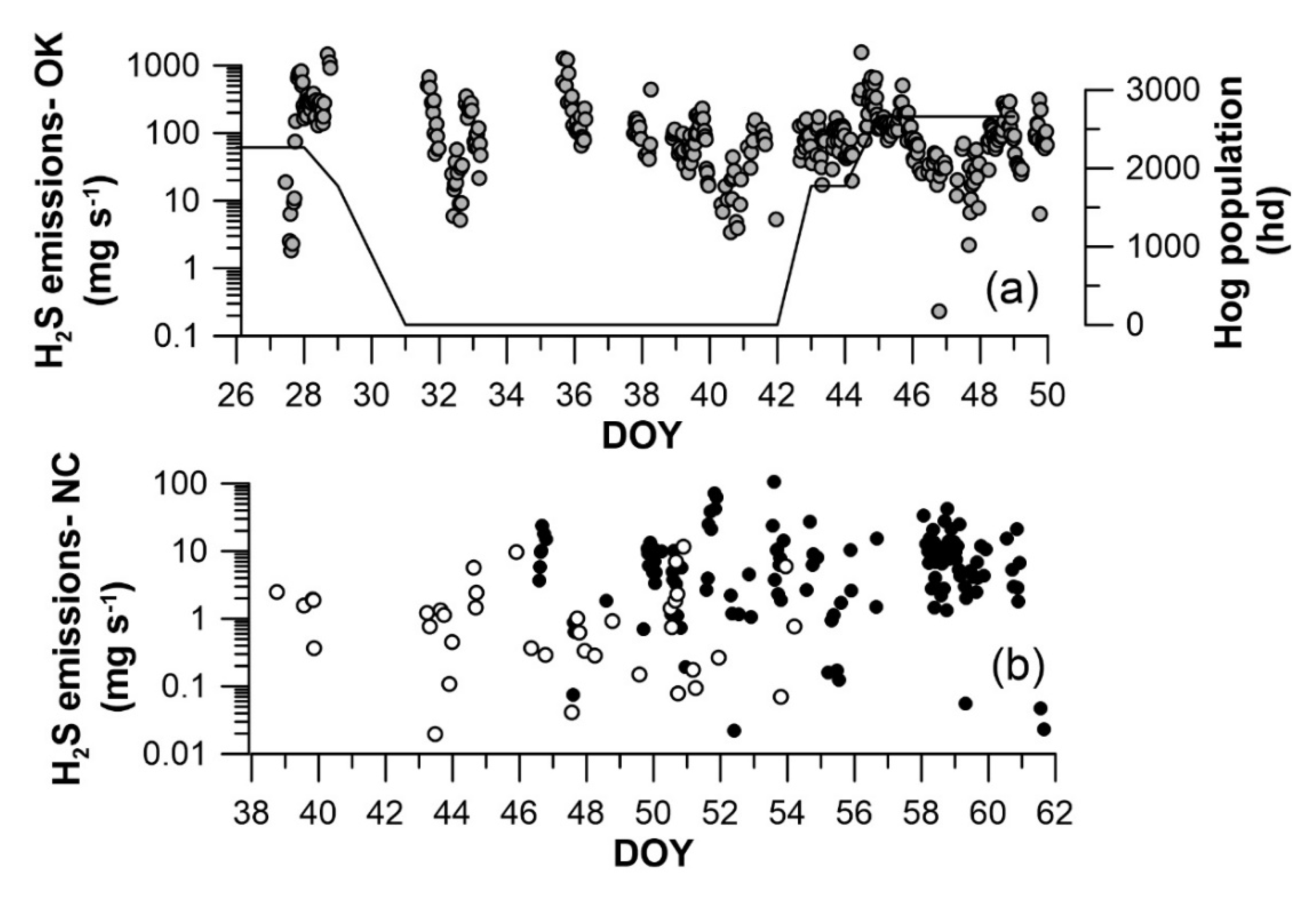
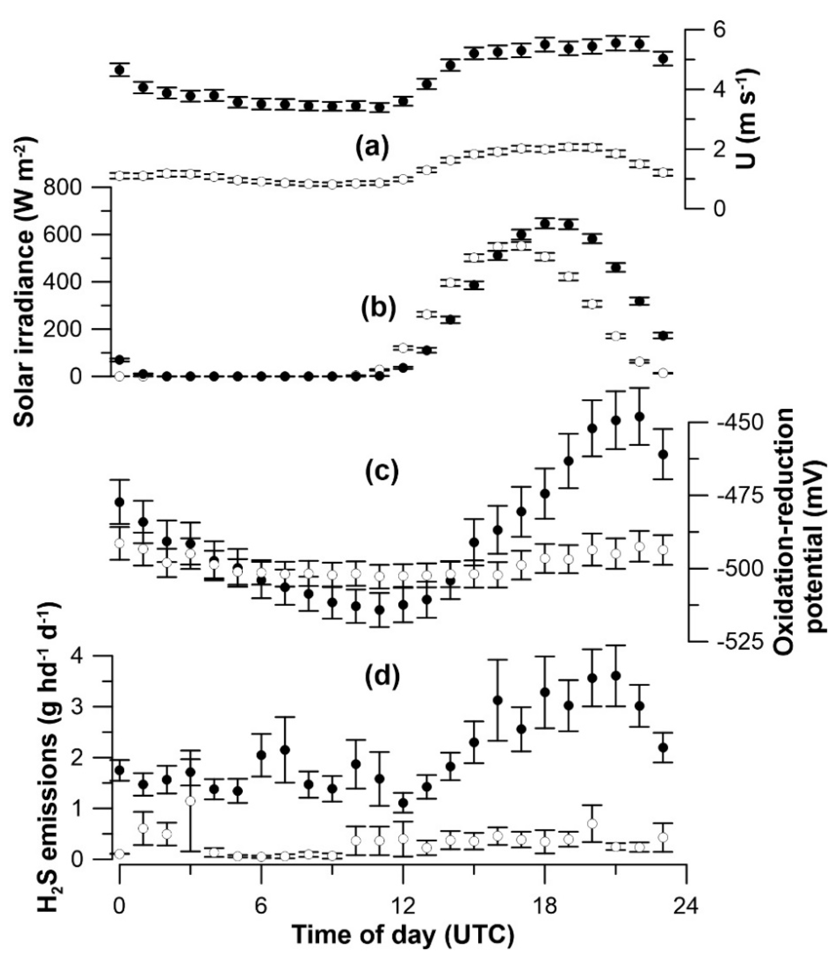
3.4. Half-Hourly Emissions

Emissions were generally greater in the first half of the year at both lagoons (Figure 3a,c). Emissions were also strongly positively skewed at both lagoons (Figure 3b,d). The mean measured emission at the NC lagoon was 9.59 mg H2S s−1 (0.53 µg H2S m−2 s−1) while the median emission was 0.14 mg H2S s−1 (0.01 µg H2S m−2 s−1). The mean measured emission at the OK lagoon was 49.99 mg H2S s−1 (5.12 µg H2S m−2 s−1) while the median emission was 11.68 mg H2S s−1 (1.20 µg H2S m−2 s−1). Emissions at the NC lagoon were more commonly near zero than at the OK lagoon (Figure 3b,d), with 657 of the 1160 measurements at the NC lagoon and 2936 of the 3527 measurements at the OK lagoon above zero. Considering only positive emissions, the mean emissions at the NC lagoon were 18.69 mg s−1 (1.04 µg H2S m−2 s−1) while those at the OK lagoon were 62.79 mg H2S s−1 (6.43 µg H2S m−2 s−1). The 90th percentile of emissions at the NC lagoon was 46.30 mg H2S s−1 (2.57 µg H2S m−2 s−1) while that at the OK lagoon was 163.30 mg s−1 (16.72 µg H2S m−2 s−1).
Low daily mean emissions may have been partly a result of the biological activity of large PSB populations in the lagoon. Again, using the coloration of the lagoon as an indicator of PSB populations, half-hourly emissions were segregated. There were 319 of the 657 positive emissions measurements without evident PSB presence at the NC lagoon and 2285 of the 2936 positive emissions measurements without evident PSB presence at the OK lagoon. The mean positive emissions at the NC lagoon when no PSB were evident was 31.40 mg H2S s−1 (1.75 µg H2S m−2 s−1) while the median emission was 9.07 mg H2S s−1 (0.50 µg H2S m−2 s−1). The mean positive emissions at the OK lagoon when no PSB were evident was 78.60 mg H2S s−1 (8.05 µg H2S m−2 s−1) while the median emission was 39.55 mg H2S s−1 (4.05 µg H2S m−2 s−1).
It was assumed previously that the mean animal population at each farm was more representative of the lagoon emissions than any individual animal population count. This was evaluated by comparing emissions over periods in which the hogs were removed from the building for sale or destruction. When the animals were removed from the buildings the pits under the buildings were flushed. At the NC operation, disease resulted in all animals being removed from the buildings and the buildings being cleaned (Table 1). At the OK operation, the three barns were sequentially emptied for hog sales with a period in which the barns were cleaned for the next cohort (Table 1). These events provided opportunities for assessment of whether the loading of the lagoon by fresh manure influenced the lagoon emissions. It was hypothesized that since H2S is produced from the sludge at depth in the lagoons, the absence of fresh manure loading would not affect the lagoon emissions.
The depopulation of the OK barns occurred over a relatively short period of time, with the barns being entirely empty for only 11 days (Table 1). Winds were nearly constant during the entire period with (n = 14; mean wind speed 4.9 m s−1) and without (n = 12; mean wind speed 4.8 m s−1) hogs present. No measurements of lagoon conditions were made as this occurred during the winter when icing was present (Table 2). Emissions during this period illustrated distinct diurnal tendencies (discussed further below) (Figure 4a). The mean half-hour H2S emissions were not significantly different between measurements made with (mean 161.3 mg s−1) or without (mean 148.5 mg H2S s−1) hogs present (Mann–Whitney test; W = 46, p = 0.63).
The NC barns were empty for an entire measurement period in 2009 (Table 1). A comparison between measurements during this period and measurements made during a similar period in 2008 provided a means of assessing the influence of fresh manure loading on lagoon emissions (Figure 4b). Mean half-hour emissions during the 2008 period when animals were present were 9.8 mg H2S s−1. Mean half-hour emissions during the 2009 period when animals were not present were 1.6 H2S mg s−1. The emissions were significantly different between the two periods (Mann–Whitney test; W = 115, p = 0.001). This difference, however, may have been at least partly due to differences in the lagoon conditions. Mean lagoon pH during the 2008 period with hogs present was 7.5 while that in 2009 when no animals were present was 8.3. Mean lagoon ORP during the 2008 period when hogs were present was −479 mV while that in 2009 when no hogs were present was −331 mV. The weaker reducing environment in 2009 suggested that PSB may have been present, contributing to the lower H2S emissions at the NC lagoons and not a lack of fresh manure loading. Wind speeds and temperatures during the two periods were similar: 1.9 m s−1 (hogs present) and 2.0 m s−1 (hogs absent) and 13 °C (hogs present) and 12 °C (hogs absent).
Analysis of the OK lagoon therefore indicated that lagoon H2S emissions were not significantly influenced by the contribution of fresh manure into the anaerobic lagoons. This supports using the mean hog population over the two years of the study for the estimation of animal-specific emission. However, the comparison of H2S emissions at the NC farm with and without hogs in the barns during a similar period of the year but different years indicated statistically significant differences in emissions. Since the comparison is made based on emissions in different years, the significant differences at the NC farm may have been due to the differences in lagoon microbial populations.
Emissions at both the NC and OK lagoons were higher during the day than during the night (Figure 5d). Wind speeds typically increased at both lagoons as the sun came up (Figure 5a,b). The timing of the increase in wind speed corresponded to increased emissions at the OK lagoon (Figure 5a,d). This was not as evident at the NC lagoon (Figure 5a,d). Increased emissions with increased wind speeds may have been partly a result of enhanced mixing in the lagoon. There were diurnal variations in emissions and ORP for the OK lagoon but not the NC lagoon (Figure 5c). The correspondence of decreasing ORP with increasing solar radiation suggested the presence of either non-detectible PSB and/or other photosynthetic organisms such as algae. Since emissions increased as ORP decreased (Figure 5c,d), the increased emissions were likely not related to low population PSB activity. It is proposed that the reduced ORP (oxygenated water) from the surface of the lagoon may have been mixed in the afternoon due to winds at the OK lagoon, but that wind speeds were too low to substantially mix the top 0.3 m depth of the NC lagoon. Given the higher winds at the OK lagoon, the lack of evidence of oxidation in the lagoon associated with the possible high PSB populations (Table 3) and the correlation of increasing emissions with increasing ORP, the higher emissions were likely due to an overwhelming influence of the shear-driven mixing on the ORP at the OK lagoon.

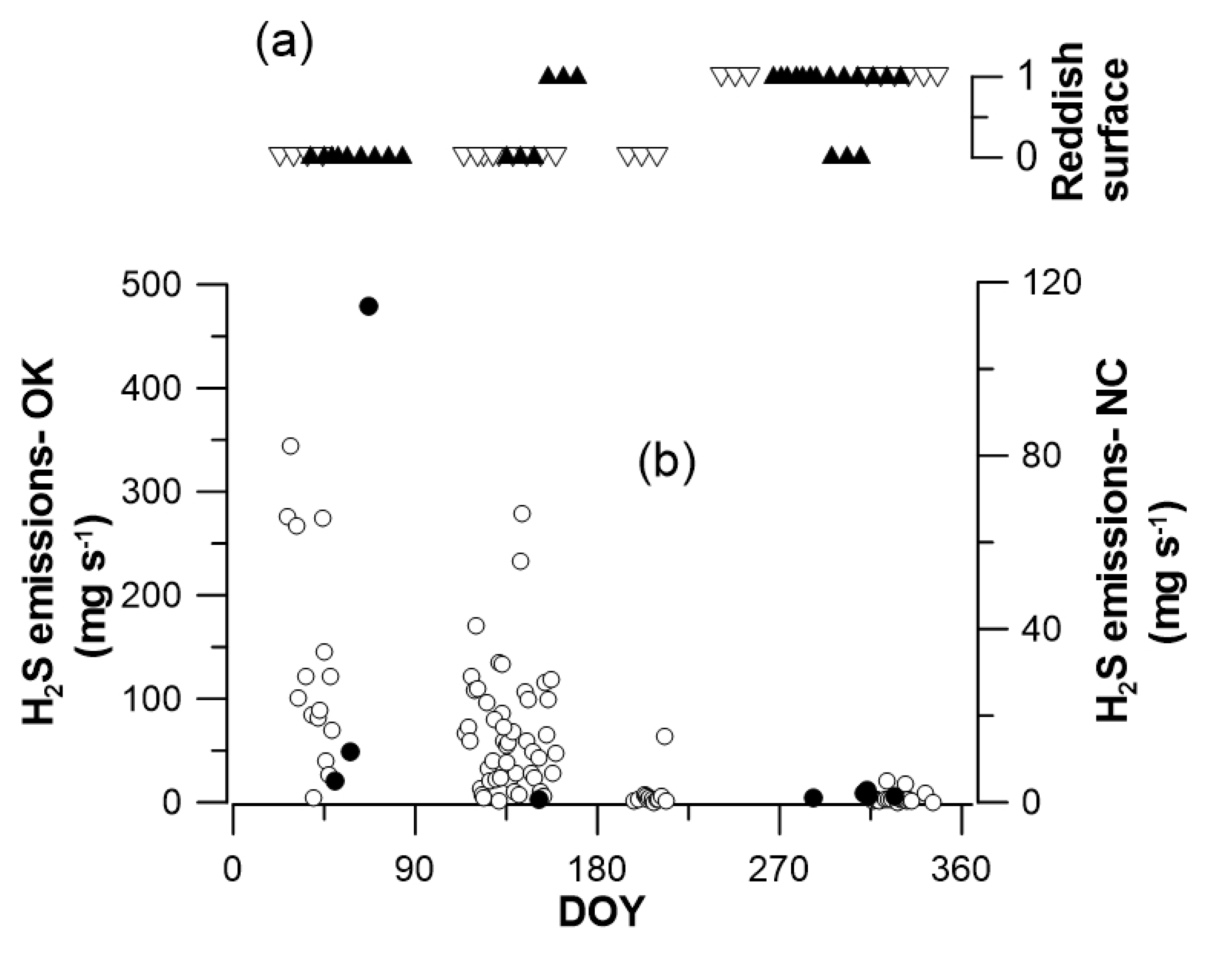
3.5. Daily Emissions

Since the distributions of the half-hourly emissions at both lagoons were strongly skewed (Figure 3b,d), emission error estimates were based on the percent error described in the methods and not on the standard deviation of the measurements. Daily emissions for representative days (with 30% error) were based on at least 11 h of valid half-hourly emission measurements at the NC lagoon (9 of the 144 days of measurements) and at least 6 h of valid half-hourly emission measurements at the OK lagoon (110 of the 122 days of measurements).
Daily emissions at the two lagoons was characterized by low emissions on most days with occasional days of high emissions (Figure 6b). The daily emissions at the NC lagoon were more commonly near zero than at the OK lagoon. In general, daily mean emissions at the two lagoons were higher in the late winter and spring and decreased by mid-year (Figure 6b), although the specific sampling periods resulted in differences in the dominant emission season (winter for the OK lagoon and spring for the NC lagoon; Table 5). Emissions from the OK lagoon were greater than those from the NC lagoon even though there were more animals at the NC farm than the OK farm.
The mean daily emission for representative days at the NC lagoon was 1.35 kg H2S d−1 ± 0.135 kg H2S d−1. The mean daily emission for representative days at the OK lagoon was 4.70 kg H2S d−1 ± 0.13 kg H2S d−1. The 90th percentile daily emissions at the NC and OK lagoons, respectively, were 5.8 kg H2S d−1 and 11.5 H2S d−1. The 90th percentile emission at the NC lagoon was 33 times the median value, while only 5 times the median value at the OK lagoon. The maximum daily emission at the NC lagoon was 9.9 kg H2S d−1. The maximum daily emission at the OK lagoon was 29.8 kg H2S d−1. The maximum daily emissions at both lagoons were below the EPCRA and CERCLA threshold for reporting of 45.4 kg H2S d−1.

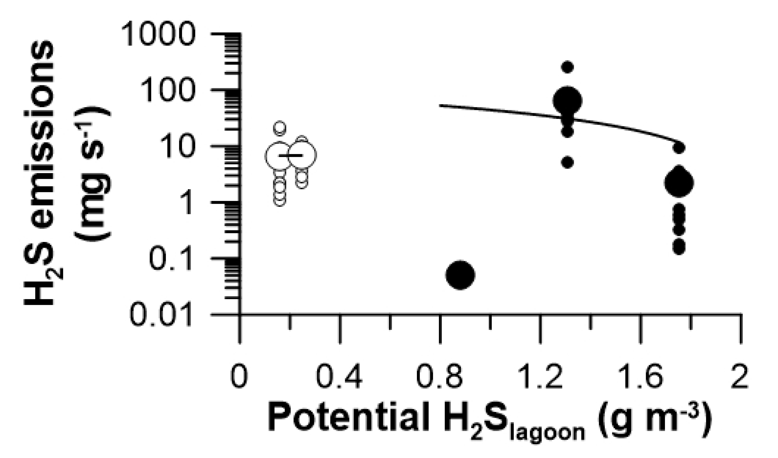
3.6. Influence of Lagoon Sulfur Content on Emissions

The decrease in emissions during the year appeared to correlate with the appearance of a reddish color on the lagoon surfaces both in NC and OK (Figure 6). Emissions are driven both by concentration gradients between the lagoon surface and the atmosphere as well as the efficiency of transport from the lagoon to the overlying air. Assuming the well-mixed lagoon liquid concentrations were representative of the surface liquid and could be considered constant at the resolution of the measurements over ± 5 days of the lagoon sample, H2S emissions on the days of lagoon sampling were compared to the estimated potential liquid H2S concentrations (Table 4). Since the background concentration of H2S in the air for the days described was less than 2.5 µg H2S m−3 and the potential liquid concentrations of H2S were 0.2 and 1.8 g H2S m−3 for the OK and NC lagoons, respectively, the H2S gradient was essentially the liquid concentration. The limited measurements (19 days) indicated the potential lagoon H2S concentration in the OK lagoon was not positively correlated with emissions (Pearson R < 0.01) (Figure 7). The NC potential lagoon H2S concentrations and the emissions (30 days) were also not positively correlated statistically (Pearson R = 0.22) due to the few days of measurements at 0.88 g H2S m−3 (Figure 7).

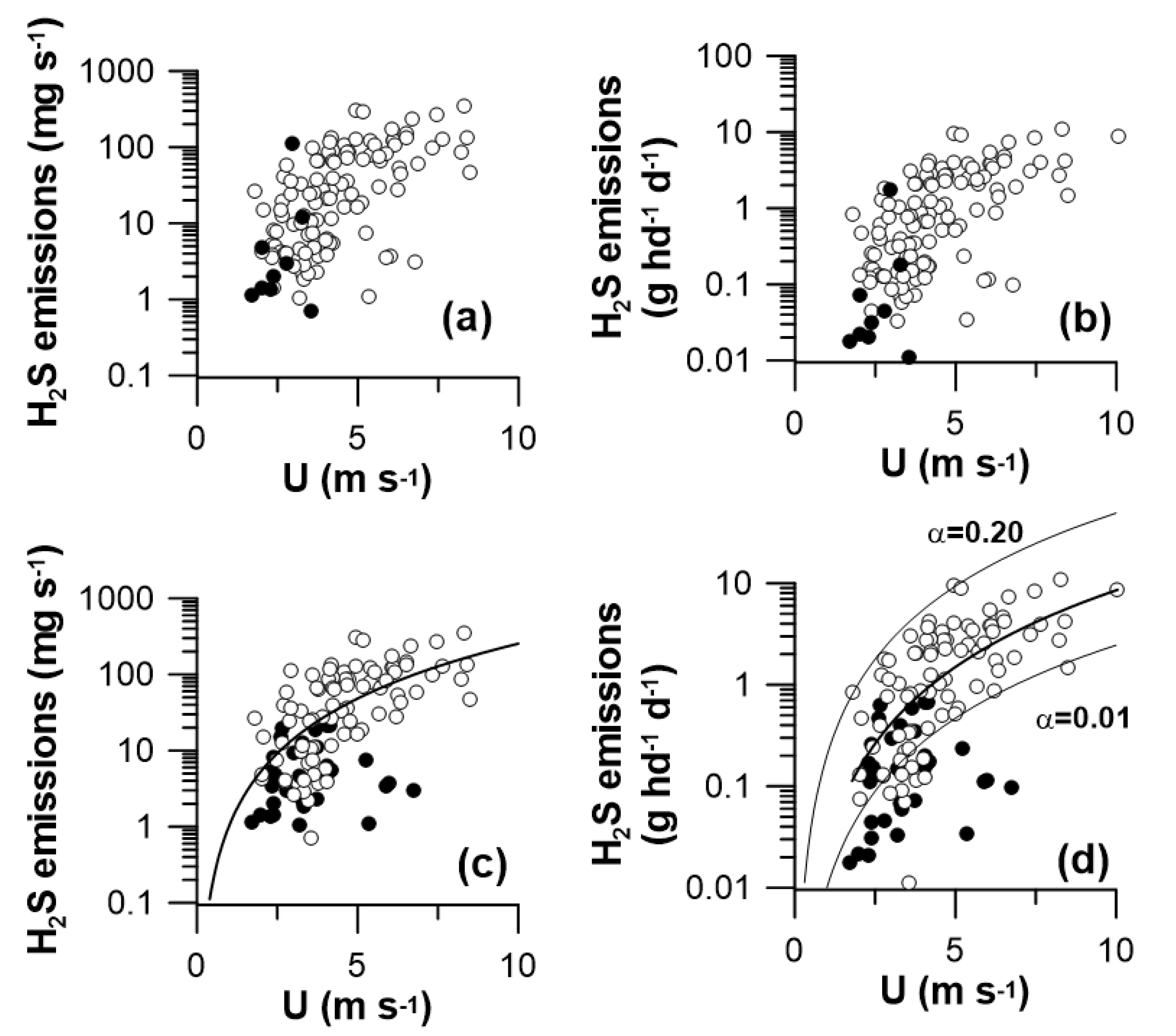
3.7. Influence of Wind on Emissions

Daily mean H2S emissions from representative days at the NC and OK lagoons showed a tendency for increased emissions with increased wind speed (Figure 8a,b). However, the range in emissions for wind speeds less than approximately 7 ms−1 was nearly constant and large. This might be expected if the PSB biological activity in the lagoons influenced the lagoon H2S emissions and the amount of biological activity varied over the study period as indicated by the reddish coloration. Daily mean H2S emissions from representative days with no evident PSB were related to wind speed and friction velocity as a power law function (Equation (1)) to describe emissions (Figure 8c,d) as used for lagoons at sow hog operations [8]. The daily mean emissions variability explained by wind speed and friction velocity, respectively, at the NC lagoon were 24% and 15% (R2 of 0.24 and 0.15). This apparent influence on emissions was much greater than the 4% reported for a sow farm in NC [8]. The daily mean emissions variability explained by wind speed and friction velocity, respectively, at the OK lagoon were 20% and 10% (R2 of 0.20 and 0.10). This apparent influence was comparable to the 25% variability explanation of daily mean emission reported for a sow farm in OK [8].
Given the large difference in hog populations between the two farms, emissions for the two farms were normalized by animal populations, combined, and then related to wind speed. A power law of daily emissions when the lagoon did not have apparent PSB populations was regressed against on wind speed (Equation (1)). The power law relationship (Equation (1)) between U and lagoon emissions in the absence of evidence of PSB had an R2 of 0.33 with an α of 1.24 mg H2S s−1 and a β of 2.23 (Figure 8c). The emissions β coefficient was similar to the average β of 1.8 reported for oxygen of water bodies [29]. The power law relationship between U and animal-basis lagoon emissions in the absence of evidence of PSB had an R2 of 0.35 with an α of 0.032 g H2S d−1 hd−1 and a β of 2.40 (Figure 8d). Assuming the source strength was varying as a result of changes in the lagoon, the range in emissions for a given wind speed was defined by using the same β coefficients and adjusting the α for the upper and lower bounds of the daily emissions when PSB were likely and unlikely (Figure 8d).
The normalized emissions (Equation (2)) of the non-reddish (no-PSB) NC and OK lagoons both fit the relationship of wind speed to the normalized emissions (Figure 9). This indicated that the lower emissions of the NC lagoon when PSB were not evident were likely primarily due to the differences in wind speeds at the two lagoons. The wind speed at the MN lagoon ranged from 1.6 to 7 ms−1 [9] while wind speed at the NC lagoon ranged from 1.0 to 2.5 ms−1 [11]. The direction of influence of wind speed on emissions is consistent with the power function indicated in Figure 8. Wind speeds at the MO lagoon where emissions were also measured were unfortunately not reported [10].
The apparent influence of lagoon temperature on normalized emissions differed depending on the evidence of PSB populations in the lagoons. A lack of influence of wind speed on emissions was suggested for days with PSB populations (Figure 8c,d). This lack of influence resulted in negative values of normalized animal-based emissions and was interpreted as evidence of PSB activity in the lagoon.
There was evidence of large PSB populations (reddish color occurred across days with 0.3 m lagoon temperatures of 3 °C to 15 °C) (Figure 9a). The optimal temperature range for PSB population growth was reported as 16 °C to 30 °C [7]. This suggests that the reddish color of the lagoon surface did not necessarily indicate high populations of PSB within the upper 0.3 m of the lagoon at the time of the measurements. PSB growth could have occurred during the gap in the measurements (Figure 3) when lagoon temperatures were more in the optimal range. The PSB population could have grown over the previous couple months.
The association of non-PSB normalized emissions with lagoon temperature suggests there is a range of temperatures in which H2S production and emission exceeded consumption by any PSB population. Negative normalized emissions were most prevalent when lagoon temperatures were above 25 °C and below 16 °C, but negative emissions were measured throughout the range of temperatures (Figure 9a). Since the optimal temperature range for PSB population growth was reported as 16 °C to 30 °C [7], there were likely days of emissions in which the PSB populations were present but not sufficiently high for reddish coloring of the liquid.
The ORP during days with reddish lagoon surface coloring spanned a ranged from −550 mV to −250 mV (Figure 9b). The apparent reddish coloring of the surface with a strongly reducing environment of less than −400 mV at the 0.3 m depth, combined with the lagoon temperatures suggested that the PSB activity (and observed liquid color) was at a greater depth than 0.3 m.
Normalized lagoon emissions when PSB populations were not evident were associated with lagoon ORP (Figure 9d). There appeared to be a threshold of lagoon ORP above which all normalized emissions were negative (Figure 9d). Remembering that the normalized emissions were based on emission measurements during days in which there were no evident PSB populations in the surface layer of the lagoons, negative emissions would imply activity of PSB without evident reddish coloring of the surface liquid layer. Using a threshold of approximately −450 mV ORP, there were ten days of emissions at the NC lagoon and seven days at the OK lagoon in which PSB appeared to strongly influence the lagoon emissions but that the population of PSB was below the visual threshold of detecting the reddish coloring. The day on which the daily normalized emissions were negative and the ORP was above the threshold at the NC lagoon was DOY 44 (Figure 6). Other days with fewer than 22 measurements (11 h) included DOY 39, 40, 45, 47, 48, 49, 51 and 65. This suggests that PSB activity at the NC lagoon continued to occur into the late winter with PSB populations that were no longer evident by a reddish lagoon surface color. These days include most of the days in which the hog barns were empty (discussed above). The days in which the daily normalized emissions were negative and the ORP was above the threshold at the OK lagoon were DOY 159, 160, 198, 200 and 201 (Figure 6). This suggests that PSB activity at the OK lagoon began to occur earlier in the summer than visually indicated by the reddish lagoon surface color.

3.8. Seasonal and Annual Emissions

The median annual emissions for both lagoons were lower than the mean annual emissions. The mean annual emissions for the NC lagoon were 23.8 mg H2S s−1 (Table 5), corresponding to 0.75 g H2S hd−1 d−1. The seasonal mean daily NC lagoon emissions during winter and summer were similar to that measured in those seasons at other NC finisher hog lagoons [11]. Measured fall NC lagoon emissions were less than the mean emissions measured in the fall at the Type 1 lagoon (6.9 mg s−1) while the OH lagoon emissions were similar (Table 5) [27].
The mean annual emissions for the OK lagoon were 67.2 mg H2S s−1 (Table 5), corresponding to 1.92 g H2S hd−1 d−1. The seasonal mean daily OK lagoon emissions during summer and fall corresponded well with emission rates of 1.57 g H2S hd−1 d−1 in late summer and early fall in Missouri [9] and 1.70 and 2.73 g H2S hd−1 d−1 in late spring to early summer for three lagoons in Minnesota [10]. The contrast between the emissions reported for lagoons in NC and those reported for lagoons in MO, MN and OK was evident.
The mean annual daily emission at the NC lagoon of 1.32 µg H2S m−2 s−1 ± 0.07 µg H2S m−2 s−1 (Table 4) was slightly less than the mean daily emission based on representative days (1.39 kg H2S d−1 ± 0.14 kg H2S d−1). Both mean values were within the error bounds of the two estimates. The mean annual daily emission at the OK lagoon of 6.88 µg H2S m−2 s−1 ± 0.13 µg H2S m−2 s−1 (Table 4) was higher than the mean daily emission at the OK lagoon based on representative days (5.09 kg H2S d−1 ± 0.15 kg H2S d−1). The mean annual daily emission was higher than the upper bound of the daily emission based on representative days (5.24 kg H2S d−1). The difference between these two estimates of the mean daily emissions was likely due to a relatively small sampling of summer emissions resulting in a negative bias to the mean daily emissions based on representative days. The best estimate of the mean annual daily emission was, therefore, the higher value where the fewer measurements during the summer are not biasing the annual emissions (Table 5).

4. Conclusions

Hydrogen sulfide emission at the NC and OK lagoons differed substantially. On the basis of the lagoon area, emissions were much higher for the OK lagoon (6.88 µg H2S m−2 s−1 ± 0.13 µg H2S m−2 s−1) than for the NC lagoon (1.32 µg H2S m−2 s−1 ± 0.07 µg H2S m−2 s−1). Fresh manure loading did not appear to influence the lagoon H2S emissions. Mean annual hog-specific emissions for the NC lagoon were 0.75 g H2S hd−1 d−1 while those for the OK lagoon were 1.92 g H2S hd−1 d−1. Wind speeds strongly influenced emissions and largely accounted for emission differences at the two lagoons when a reddish color on the lagoon surface, suggesting a low or absent PSB population, was not evident. The relationship of normalized emissions to ORP suggests that PSB were present and influencing emissions when the lagoon surface was not clearly reddish. Although the appearance of a reddish surface in the late spring and summer corresponded with decreased emissions at both lagoons, evidence that the reddish color corresponding with PSB activity was weak. Oxidation during the daytime at the OK lagoon was likely largely associated with wind shear mixing and not PSB activity. Since the wind speeds at the NC lagoon were usually low, the oxidation in the NC lagoon was likely to be mostly a result of PSB activity.

Author Contributions

Conceptualization, R.H.G.; methodology, R.H.G.; software, M.T.B.; validation, M.T.B. and R.H.G.; formal analysis, R.H.G. and M.T.B.; investigation, R.H.G.; resources, R.H.G.; data curation, M.T.B. and R.H.G.; writing—original draft preparation, R.H.G.; writing—review and editing, R.H.G. and M.T.B.; visualization, R.H.G.; supervision, R.H.G.; project administration, R.H.G.; funding acquisition, R.H.G. All authors have read and agreed to the published version of the manuscript.

Funding

This research was funded by livestock producers, the Agricultural Air Research Council, Inc., and National Pork Producers.

Institutional Review Board Statement

Not applicable.

Informed Consent Statement

Not applicable.

Data Availability Statement

Daily data is publicly available and can be found at: https://archive.epa.gov/airquality/afo2012/web/html/ok3a.html, accessed on 19 December 2019 and https://archive.epa.gov/airquality/afo2012/web/html/nc3a.html, accessed on 19 December 2019. Half-hourly data presented in this study are available on request from the corresponding author.

Acknowledgments

Assistance with field measurements was made by A. Lawrence, J. Wolf, S. Cortus, C. Fullerton and D. Snyder. Without their help, this work could not have been possible.

Conflicts of Interest

The authors declare no conflict of interest. The funders had no role in the design of the study; in the collection, analyses, or interpretation of data; in the writing of the manuscript, or in the decision to publish the results.

References

  1. Grant, R.H.; Boehm, M.T.; Lawrence, A.J.; Heber, A.J.; Wolf, J.M.; Cortus, S.D.; Bogan, B.W.; Ramirez-Dorronsoro, J.C.; Diehl, C.A. Methodologies of the National Air Emissions Measurement Study Open Source Component. In Proceedings of the Symposium on Air Quality Measurement Methods and Technology, Chapel Hill, NC, USA, 3–6 November 2008; Air and Waste Management Association: Durham, NC, USA, 2008. [Google Scholar]
  2. Clanton, C.J.; Schmidt, D.R. Sulfur compounds in gases emitted from stored manure. Trans. ASAE 2000, 43, 1229–1239. [Google Scholar] [CrossRef]
  3. Hamilton, D.W.; Fathepure, B.; Fulhage, C.D.; Clarkson, W.; Lalman, J. Treatment lagoons for animal agriculture. In Animal Agriculture and the Environment; Rice, J.M., Caldwell, F., Humanik, F.J., Eds.; White Paper; National Center for Manure and Animal Waste Management: St. Joseph, MI, USA, 2006; pp. 547–573. [Google Scholar]
  4. Ni, J.-Q.; Heber, A.J.; Sutton, A.L.; Kelly, D.T. Mechanisms of gas releases from swine wastes. Trans. ASABE 2009, 52, 2013–2025. [Google Scholar]
  5. Chen, T.; Schulte, D.D.; Koelsch, R.K.; Parkhurst, A.M. Characteristics of phototrophic and non-phototrophic lagoons for swine manure. Trans. ASABE 2003, 46, 1285–1292. [Google Scholar] [CrossRef]
  6. Van Gemerden, H.; Mas, J. Ecology of phototrophic sulfur bacteria. In Anoxygenic Photosynthetic Bacteria; Blankenship, R.E., Madigan, M.T., Bauer, C.E., Eds.; Kluwer Academic: Dordrecht, The Netherlands, 1995; pp. 49–85. [Google Scholar]
  7. Holm, H.W.; Vennes, J.W. Occurrence of purple sulfur bacteria in a sewage treatment lagoon. Appl. Microbiol. 1970, 19, 988–996. [Google Scholar] [CrossRef] [PubMed]
  8. Grant, R.H.; Boehm, M.T.; Lawrence, A.J.; Heber, A.J. Hydrogen sulfide emissions from sow farm lagoons along a climate continuum. J. Environ. Qual. 2013, 42, 1674–1683. [Google Scholar] [CrossRef] [PubMed]
  9. Zahn, J.A.; Tung, A.E.; Roberts, B.A. Continuous ammonia and hydrogen sulfide emissions measurements over a period of four seasons from a central Missouri swine lagoon. In Proceedings of the ASAE Annual International Meeting, Nashville, TN, USA, 20–23 August 2022; p. 024080. [Google Scholar]
  10. Bicudo, J.R.; Clanton, C.J.; Schmidt, D.R.; Powers, W.J.; Jacobson, L.W.; Tengman, C.L. Geotextile covers to reduce odor and gas emissions from swine manure storage ponds. Appl. Eng. Agric. 2004, 20, 65–75. [Google Scholar] [CrossRef]
  11. Blunden, J.; Aneja, V.P. Characterizing ammonia and hydrogen sulfide emissions from a swine waste treatment lagoon in North Carolina. Atmos. Environ. 2008, 42, 3277–3290. [Google Scholar] [CrossRef]
  12. Grant, R.H.; Boehm, M.T. National Air Emissions Monitoring Study: Data from the Southeastern US Pork Production Facility NC3A.; Final Report to the Agricultural Air Research Council; Purdue University: West Lafayette, IN, USA, 2010. Available online: www.epa.gov/airquality/agmonitoring/nc3a.html (accessed on 25 March 2013).
  13. Heber, A.J.; Ni, J.-Q.; Haymore, B.L.; Duggirala, R.K.; Keener, K.M. Air quality and emission measurement methodology at swine finishing buildings. Trans. ASAE 2001, 44, 1765–1778. [Google Scholar] [CrossRef]
  14. APHA. Method 4500-H+ A: pH value. In Standard Methods for the Examination of Water and Wastewater, 19th ed.; Eaton, A.D., Clesceri, L.S., Greenberg, A.E., Eds.; American Waste Water Association: Denver, CO, USA, 1995; pp. 465–469. [Google Scholar]
  15. APHA. Method 2590 B: Oxidation–reduction potential in clean water. In Standard Methods for the Examination of Water and Wastewater, 19th ed.; Eaton, A.D., Clesceri, L.S., Greenberg, A.E., Eds.; American Waste Water Association: Denver, CO, USA, 1995; pp. 273–277. [Google Scholar]
  16. USEPA. Revised National Pollutant Discharge Elimination System Permit Regulation and Effluent Limitations Guidelines for Concentrated Animal Feeding Operations in Response to the Waterkeeper Decision; Final Rule. Part II, 40 CFR Parts 9, 122, and 412; USEPA: Washington, DC, USA, 2008.
  17. Trabue, S.L.; Kerr, B.J.; Scoggin, K.D. Swine diets impact manure characteristics and gas emissions: Part I sulfur level. Sci. Total Environ. 2019, 687, 800–807. [Google Scholar] [CrossRef] [PubMed]
  18. Trabue, S.L.; Kerr, B.J.; Scoggin, K.D. Swine diets impact manure characteristics and gas emissions: Part II sulfur source. Sci. Total Environ. 2019, 689, 1115–1124. [Google Scholar] [CrossRef] [PubMed]
  19. Madigan, M.T.; Jung, D.O. An overview of purple bacteria: Systematics, physiology and habitats. In The Purple Phototrophic Bacteria. Advances in Photosynthesis and Respiration; Hunter, C.N., Daldal, F., Thurnauer, M.C., Beatty, J.T., Eds.; Springer: London, UK, 2009; Volume 28, pp. 2–15. [Google Scholar]
  20. Flesch, T.K.; Wilson, J.D.; Harper, L.A.; Crenna, B.P. Estimating farm emissions of ammonia with an inverse dispersion technique. Atmos. Environ. 2005, 39, 4863–4874. [Google Scholar] [CrossRef]
  21. Flesch, T.K.; Wilson, J.D.; Harper, L.A.; Crenna, B.P.; Sharpe, R.P. Deducing ground-to-air emissions from observed trace gas concentrations: A field trial. J. Appl. Meteorol. 2004, 43, 487–502. [Google Scholar] [CrossRef] [Green Version]
  22. Laubach, J.; Kelliher, F.A. Measuring methane emission rates of a dairy cowherd (II): Results from a backward-Lagrangian stochastic model. Agric. For. Meteorol. 2005, 129, 137–150. [Google Scholar] [CrossRef]
  23. Gao, Z.; Desjardins, R.L.; van Haarlem, R.P.; Flesch, T.K. Estimating gas emissions from multiple sources using a backward lagrangian stochastic model. J. Air Waste Manag. Assoc. 2008, 58, 1415–1421. [Google Scholar] [CrossRef] [PubMed]
  24. Blair, R.C.; Higgins, J.J. Comparison of the power of the paired samples t test to that of Wilcoxon’s signed-ranks test under various population shapes. Psychol. Bull. 1985, 97, 119–128. [Google Scholar] [CrossRef]
  25. Grant, R.H.; Mangan, M.R.; Boehm, M.T. Variability in H2S emissions from a midwestern dairy lagoon. J. Environ. Qual. 2021, 50, 1063–1073. [Google Scholar] [CrossRef] [PubMed]
  26. Peters, J.; Combs, S.; Hoskins, B.; Jarman, J.; Kovar, J.; Watson, M.; Wolf, A.; Wolf, N. Recommended Methods of Manure Analysis; University of Wisconsin Cooperative Extension Publishing: Madison, WI, USA, 2003. [Google Scholar]
  27. Zahn, J.A.; Hatfield, J.L.; Laird, D.A.; Hart, T.T.; Do, Y.S.; DiSpirito, A.A. Functional classification of swine manure management systems based on effluent and gas emissions characteristics. J. Environ. Qual. 2001, 30, 635–647. [Google Scholar] [CrossRef] [PubMed] [Green Version]
  28. Sund, J.L.; Evenson, C.J.; Strevett, K.A.; Nairn, R.W.; Athay, D.; Trawinski, E. Nutrient conversions by photosynthetic bacteria in a concentrated animal feeding operation lagoon system. J. Environ. Qual. 2001, 30, 648–655. [Google Scholar] [CrossRef] [PubMed]
  29. Ro, K.S.; Hunt, P.G. A new unified equation for wind-driven surficial oxygen transfer into stationary water bodies. Trans. ASABE 2006, 49, 1615–1622. [Google Scholar]
Figure 1. Lagoon and measurement configurations. The measurement configurations at the NC lagoon (a) and OK lagoon (b). Solid white lines indicate locations of S-OPS while white circles and ‘x’ indicate the locations of the meteorological and lagoon measurements respectively.
Atmosphere 13 00153 g001
Figure 2. Oxidation-reduction potential: (a) The relationship of daily mean lagoon temperature to oxidation-reduction potential in NC (filled circles) and OK (open circles) lagoons; (b) The relationship of daily mean solar radiation to oxidation-reduction potential in NC (filled circles) and OK (open circles) lagoons. Conditions conducive to PSB development is indicated by boxed region.
Atmosphere 13 00153 g002
Figure 3. Half-hourly emissions at the two lagoons: (a) Annual variation in H2S emissions at the NC lagoon; (b) Frequency distribution of half-hourly emission measurements at the NC lagoon; (c) Annual variation in H2S emissions at the OK lagoon; (d) Frequency distribution of half-hourly emission measurements at the NC lagoon.
Atmosphere 13 00153 g003
Figure 4. Influence of fresh manure loading on half-hourly lagoon emissions: (a) Variation in H2S emissions with population (solid line) of the three barns; (b) Variation in H2S emissions with (solid circles) and without (open circles) hogs in the barns.
Atmosphere 13 00153 g004
Figure 5. The diurnal variation in winds, solar radiation, ORP and mean emissions when the lagoon was not reddish (no evidence of PSB). The hourly mean values with error bars of standard error of the mean for the NC (open circles) and OK (filled circles) are indicated for the wind speed (a), solar irradiance (b), lagoon oxidation reduction potential (c) and emissions (d).
Atmosphere 13 00153 g005
Figure 6. Annual variation in daily emissions (representative days) and observed lagoon coloration: (a) The daily lagoon surface color; (b) H2S emissions. Values are indicated for the NC lagoon (closed symbols) and OK lagoon (open symbols).
Atmosphere 13 00153 g006
Figure 7. Relationship between potential lagoon liquid H2S concentration and H2S emissions. The daily mean half-hour emissions for the NC (filled circle) and OK (open circle) lagoons are indicated relative to lagoon S concentration for ± five days of lagoon liquid concentration measurement. Large symbols indicate mean emissions for a given H2S concentration.
Atmosphere 13 00153 g007
Figure 8. Dependence of daily H2S emissions (representative days) on wind speed. The daily mean emissions for the NC (filled circle) and OK (open circle) are indicated relative to farm lagoon (a) and farm head of animals loading the lagoon (b). The daily mean animal-based emissions for the lagoon with evident PSB (filled circle) and not evident PSB (open circle) are indicated relative to farm lagoon (c) and farm head of animals loading the lagoon (d). The power function regressions of emissions on wind speed (Equation (1)) are indicated by solid line with the upper and lower bound of the power function for the non-PSB lagoon emissions indicated by the thin lines respectively.
Atmosphere 13 00153 g008
Figure 9. Normalized daily emissions for representative days without evident PSB relative to oxidation-reduction potential. The normalized animal-based daily mean values (Equation (2)) for the NC (solid circle) and OK (open circle) relative to lagoon temperature with evident PSB populations (a) and without evident PSB populations (c). The normalized animal-based daily mean values relative to lagoon ORP with evident PSB populations (b) and without evident PSB populations (d).
Atmosphere 13 00153 g009
Table 1. Producer-supplied farm activity.
FarmPeriodActivityAnimal Inventory
NC24 October–7 November 2007No events6963
13 February–5 March 2008No events5004
6–26 March 2008No events6425
25 September–14 October 200829–30 September 2008 lagoon pump-out3533
4–23 February 2009No animals present due to disease0
12 May–2 June 2009No events7126
2–22 June2009No events7063
24 September–2 December 2009No events8702
OK30 August–18 September 2007No events2267
25 September 2007All 3 barns emptied0
27 September and 4 October 2007New group of pigs restocked2267 *
24 January–19 February 200829 January 2008 North Barn emptied
30 January 2008 Middle Barn emptied
31 January 2008 South Barn emptied
11 February 2008 North & Middle restocked
14 February 2008 South Barn restocked
1773 *
887 *
0 *
1773 *
2660
7–29 May 2008No events2747
29 May–10 June 200828 May–11 June 2008 pig shipments: total of 2079 were shipped out during this period2747
4 November–3 December 2008No events2909
3–16 December 2008No events2880
21 April–14 May 2009No events2882
14 July–4 August 2009No events2845
* Estimated.
Table 2. Physical characteristics of lagoons.
FarmDate—Appearance (Color/Crust/Scum)Liquid Depth (m)Sludge Depth (m)Source of Depth Info
NC24–26 November 2007—dark/no crust or scum
7 November 2007—brown/red/no crust or scum
1.98N/A 1Producer
13–14 February 2008—black/no crust or scum
5 March 2008—black/partial scum
2.45N/AProducer
6 March 2008—black/80% scum
26–27 March 2008—brown/no crust 0–30% scum
2.57N/AProducer
24–25 September 2008—reddish/no crust or scum
14 October 2008—reddish/brown/50% film
N/AN/AN/A
4–6 February 2009—blackish/no crust
23–24 February 2009—black w/pink in corner/slight scum
2.21
1.49

0.78
Producer;
sludge gun
12–14 May 2009—black/20–30% scum2.33
1.8

0.3
Producer; sludge gun
2–3 June 2009—brown/red/80% scum
22–23 June 2009—black/40–50% scum
2.46N/AProducer
22–24 September 2009—brown/red/no crust or scum
13 October 2009—black/90% scum
26–27 October 2009—red/5% crust
10–11 November 2009—red/no crust or scum
2 December 2009—red/5% crust
N/AN/AN/A
OK30–31 August 2007—brown/red/foamy
18–19 September 2007—brown/red/0–20% crust
5.26N/AProducer
24–25 January 2008—brown/100% frozen
5–6 February 2008—brown/no crust
19 February 2008—brown/red/5% crust
5.54N/AProducer
6–8 May 2008—brown/no crust
19, 29 May 2008—brown/15% scum
5.69N/AProducer
29 May 2008 and 10 June 2008 brown/no crust5.71N/AProducer
5–7, 17 November 2008—brown/no crust, 0–5% scum
2–3 December 2008—brown/red/no crust
5.41N/AProducer
3 December 2008—brown/no crust
16 December 2008—brown/red/50% frozen
5.56N/AProducer (5 January 2009)
21–23 April 2009—brown/30% to 50% scum
6, 14 May 2009—brown/10–20% scum
5.49N/AProducer (14 April 2009)
14–16 July 2009, 4 August 2009—brown/no crustN/AN/A
1 N/A: Not available.
Table 3. In situ lagoon conditions at 0.3 m depth associated with PSB evidence.
LocationReddish Surface (PSB) Mean ORPlagoont Statistic (ORPlagoon)Mean pHlagoont Statistic (pHlagoon)
NCNot evident−504.7 7.7
Evident−462.33.6 *8.05.7 *
OKNot evident−466.6 7.7
Evident−499.5−2.4 *7.6−3.8 *
* Significant at α = 0.05.
Table 4. Liquid sample chemistry of lagoons associated with PSB evidence.
NC LagoonOK Lagoon
DatepH Maximum Possible H2S 1
(mg m−3)
Reddish Surface
(PSB Evidence)
DatepH H2S
(mg m−3)
Reddish Surface
(PSB Evidence)
20 November 20077.31796No28 November 20078.4128
25 March 20087.51307No
26 August 20087.9494No
15 October 20087.6878Yes19 November 20088.3159Yes
16 December 20087.8603No
18 February 20096.91752No
31 March 20097.9494No
21 May 20097.51307Yes
13 July 20097.6658Yes17 July 20097.9247No
1 September 20097.6658Yes
1 Estimated from S content (see methods).
Table 5. Summary of seasonal H2S emissions for the two lagoons based on all valid measurements.
SeasonNC Lagoon OK Lagoon
Count Mean (mg s−1)Mean
(µg m−2 s−1)
Mean (g/hd−1 d−1)Error (%)Count Mean (mg s−1) Mean
(µg m−2 s−1)
Mean
(g hd−1 d−1)
Error (%)
Winter1644.660.260.1511.0505148.615.224.254.6
Spring15960.263.351.9011.2133485.08.702.432.8
Summer6528.811.600.9117.553927.92.850.804.5
Fall2691.340.070.048.65587.30.740.214.4
Annual65723.771.320.755.5293667.26.881.921.9
Publisher’s Note: MDPI stays neutral with regard to jurisdictional claims in published maps and institutional affiliations.

