Article

Long-Term Analysis of Tropospheric Ozone in the Urban Area of Guadalajara, Mexico: A New Insight of an Alternative Criterion

by
José de Jesús Díaz-Torres
1,*,
Valeria Ojeda-Castillo
2,
Leonel Hernández-Mena
1,
Josefina Vergara-Sánchez
3,
Hugo Albeiro Saldarriaga-Noreña
4 and
Mario Alfonso Murillo-Tovar
5,*
1
Analytical and Metrological Services Unit, Center for Research and Assistance in Technology and Design of the State of Jalisco, 800, Normalistas Ave., Colinas de la Normal, Guadalajara 44270, Mexico
2
División de Química Aplicada, Universidad Tecnológica de Jalisco, Guadalajara 44979, Mexico
3
Escuela de Estudios Superiores de Xalostoc, Universidad Autónoma del Estado de Morelos, Av. Nicolás Bravo s/n, Parque Industrial Cuautla, Xalostoc 62717, Mexico
4
Centro de Investigaciones Químicas-IICBA, Universidad Autónoma del Estado de Morelos, Av. Universidad 1001, Col. Chamilpa, Cuernavaca 62209, Mexico
5
CONACYT-Centro de Investigaciones Químicas-IICBA, Universidad Autónoma del Estado de Morelos, Av. Universidad 1001, Col. Chamilpa, Cuernavaca 62209, Mexico
*
Authors to whom correspondence should be addressed.
Atmosphere 2022, 13(2), 152; https://doi.org/10.3390/atmos13020152
Submission received: 27 November 2021 / Revised: 12 January 2022 / Accepted: 14 January 2022 / Published: 18 January 2022
(This article belongs to the Special Issue Feature Papers in Atmosphere Science)

Abstract

:
Tropospheric ozone is an obligatorily-regulated pollutant, to ensure health protection and better air quality. Most countries have established maximum permissible limits (MPL) equal to 0.06 or 0.070 ppmv, but these could be insufficient considering the strictest MPL of the World Health Organization (WHO) guidelines. Such concentrations may still cause health damage to some groups of the population in urban areas. Additionally, the mean value is the principal statistical parameter for monitoring air pollution. This factor may be hiding critical ozone concentrations for public health. This work examines the mean and maximum ozone based on a multi-temporal analysis, to explore the use of a maximum average value as an air quality standard. The mean ozone had a remarkably stationary contrast; while, the maximum ozone emphasized a semi-permanent state of high pollution over the year. Diurnal variation highlights the differences of frequency between the mean and maximum ozone above any MPL, which is accentuated when compared with the WHO guidelines. Under the WHO-MPL, the mean ozone underestimates the highest concentrations; while the maximum ozone represents the extremely high concentrations observed over the year. Instead, the maximum average ozone becomes moderate; this preserves the proper, but conservative high concentrations, following similar temporal patterns as the mean ozone. This parameter is proposed to be adapted as an alternative statistical criterion to prevent negative effects on public health due to high and frequent ozone concentrations in subsequent years.

1. Introduction

Air pollution is the cause of 7 million premature deaths every year [1]. About 0.15 to 0.49 million of these deaths are attributable to respiratory complications by ozone [2]. Ozone is one of the main constituents of photochemical smog and a major human health concern among air pollutants [1]. Tropospheric ozone is formed through UV–photochemical atmospheric reactions involving oxygen, nitrogen oxides (NOx), and volatile organic compounds (VOCs) [3,4,5,6]. Natural sources emit ozone precursors; however, incomplete automobile combustion processes and continued industrialization related to population growth have the strongest association with increments of tropospheric ozone in megacities [7,8,9,10,11].
The persistence of high ozone concentrations in urban areas is a hazard factor that can cause severe health problems among the inhabitants. According to the WHO, there is a high probability that young people who normally breathe at least 0.060 ppmv are prone to suffer pulmonary function alterations in the short term [12,13]. While, a population exposed up to 0.080 ppmv over 6.6 h could be at risk of damage in tissues of the respiratory tract, breathing problems (inflammation, irritation, coughing, and chest tightness), asthma, and lung inflammatory reactions in the short term. In the medium and long term, ozone levels above 0.120 ppmv may produce lung function changes, lung diseases, and mortality.
The general framework indicates that the international community has made mandatory the control of tropospheric ozone and its precursors, to avoid high-pollution episodes and acute effects on human health. There have been efforts to reduce the frequency of high pollution episodes based on epidemiological evidence, as well as the establishment of ozone doses to prevent acute effects on human health [13]. Countries such as the United States have established a maximum permissible limit of 0.070 ppmv, considering the 8-h moving average values [14]; while the World Health Organization suggests an MPL of 0.050 ppmv for ozone [15]. However, none of these limits ensure absolute safety conditions [16]; because some population groups may still suffer chronic disease, either from cumulated effect or the mixture of ozone with other pollutants in the long term [12].
We took the Guadalajara Metropolitan Area (GMA) in Mexico as a study case, due to ozone constantly acting as an air pollutant, producing recurrent atmospheric contingencies during the spring–summer seasons; similar poor air quality prevails in the winter season, due to particulate matter such as PM10 or PM2.5 [17]. The maximum permissible limit (MPL) for ozone in the country was 0.080 ppmv for the 8-h moving average; in 2014, the Mexican standard was updated to 0.070 ppmv [18], as in the United States [14]. It is a limit significantly higher than the strictest limits of the WHO. There are no studies in the GMA focused on the analysis of ozone concentrations under the strictest limits of the WHO-AQGs. Instead, recent studies in the GMA analyzed a part of the long-time series given their publication date [19,20,21], these have led to a limited understanding of ozone. In a global context, the GMA is a medium-sized metropolis that may represent the type of city with high levels of pollution from ozone.
This study aims to discuss the current standard limits internationally established to control air pollution from ozone in urban areas, considering the importance of complementary analytical factors in the study of episodes of high ozone concentrations. An alternative statistical criterion is examined to evaluate air quality based on the monitoring system. The maximum average concentrations may depict the real level of this pollutant, considering a quasi-homogeneous air pollution from ozone in the city. This study emphasizes the need to adopt preventive measures against high ozone, in favor of public health for the subsequent years.

2. Materials and Methods
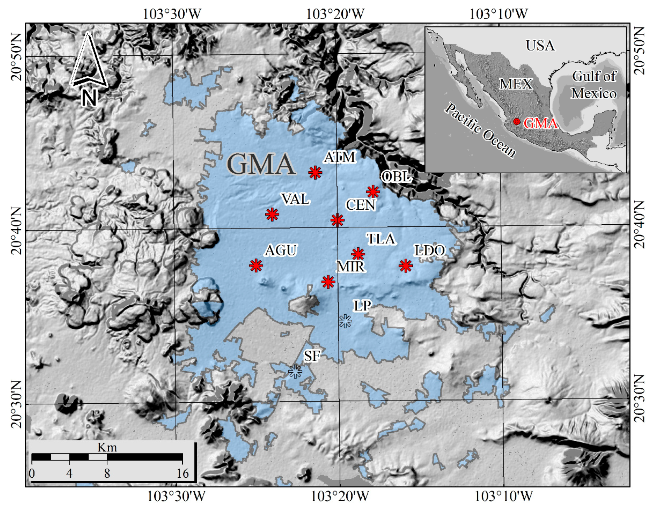
2.1. Study Area

The GMA is located at the western end of México (Figure 1). The mean elevation in the city is 1585 masl; the climate is warm and humid with a well-defined summer rain regime (June–October) [22]. Meteorological data measured in the city shows that the annual mean temperature is around 19.2 °C, with a monthly average temperature between 15.5 and 22.9 °C during the winter (January) and spring (May) seasons, respectively; meanwhile, the diurnal temperature variation is normally around 16.1 °C [23]. The average annual rainfall range is close to 866 mm, with a summer regime (June to October) having July as the rainiest month, with 225.6 mm on average. The wind direction typically is from the southeast (July to October) and southwest (December to June) [21]. The city receives high amounts of solar irradiation, with an average annual irradiance of 5.7 ± 0.9 kWh m−2 d−1 [24]. Overall, these environmental properties induce well-defined changes in the atmosphere throughout the annual cycle.
This climatic variable induces a photo-reactive atmosphere, which mainly favors the ozone formation rate during the dry–warm season (March–June), when the temperature reaches the highest values, under the lowest percentage of humidity (Figure 2). The atmospheric conditions promote the formation of photochemical smog, prevailing for large periods of the day during the dry–warm season, which is produced by mobile sources (the main cause of annual pollution). Mobile sources contribute to 85% of the total emissions in the state, with CO, VOCs, and NOx as the most abundant substances, all of them tropospheric ozone precursors. Additionally, typically, forest fires next to the city worsen the air quality of the GMA due to particulate matter.

2.2. Data Source and Quality Control

The present study focuses on information from the eight stations published with the most complete data record of the atmospheric monitoring system in the GMA, from 1996 to 2019 (Figure 1). Ozone was measured using a non-dispersive UV photometry technique using a Lear Siegler model 9810 gas analyzer, which receives scheduled preventive maintenance every three months [26]. This dataset contains more than 1.68 million records of the tropospheric ozone, averaged every 60 min. The dataset underwent a quality control process, removing invalid data related to electrical or analyzer failures, equipment maintenance, calibration, and values outside the detection limits, all following the methodology described by [27]. The ozone concentrations were analyzed with conditional functions for compliance, with a sufficiency criterion (at least 75% of the hourly and daily records) established by the Mexican Official Standard [18]. Descriptive statistics showed that all stations met the 75% sufficiency criterion, that is, eighteen hours or more in every one of the six to eight stations per day. The valid records were from 87.0 to 91.8% of the total information in almost all stations, except the Oblatos station, where 77.8% was recovered.
The hourly dataset helped us to perform an analysis of ozone concentrations in fine-scale (1-h and 8-h moving average). This was based on calculation of an index (normalized-difference ozone index) and the statistical probability; both throughout the day and considering the entire 24-year period. In addition to the hourly analysis, this dataset helped to calculate the ozone at daily and monthly resolution, to expose a broad picture of the ozone behavior. The first step was the estimation of the daily mean and maximum ozone per station; subsequently, we estimated the daily average, maximum, and maximum average values as parameters of the eight stations established in the city These parameters were aggregated at monthly scales, to analyze the seasonal variation throughout the annual cycle.

2.3. Time Series Analysis

The 1-h ozone concentrations helped to build time series with daily mean and maximum values over a period of twenty-four years [17]. Time series were used to discover normal and temporal patterns (most frequent values) of the ozone concentrations (cyclical variations, and seasonality) using seasonal decomposition method. This method involved the subtraction of the trend, cycles, and random effects, in order to understand the seasonal variation (e.g., day, month, quarter) [28]. Under seasonal decomposition, the seasonal index quantifies differences between the monthly ozone and the full period average. The index is a simple ratio to obtain a reference value (the unit) establishing proportional seasonal deviations.

2.4. The Normalized-Difference Ozone Index (NDO3I)

The normalized index for the ozone is a complementary tool to analyze its concentration; the index works as a filter based on a cut-off threshold defined by any MPL value, highlighting only those ozone measurements outside the standard limit established for any case, according to the country (Equation (1)). It is not a model that seeks to replace an air quality index for such criteria pollutant; instead, the index only shows unacceptable ozone concentrations for public health, considering the simple magnitude of the tropospheric ozone in urban areas.
N D O 3 I = O 3 , i O 3 , r O 3 , i + O 3 , r
The index reflects the difference between the absolute hourly ozone concentration (i) and an MPL value (r); while, the sum of the paired amounts normalizes such deviations. The MPL values used as thresholds were 0.050 ppmv for WHO guidelines and 0.070 ppmv for the EPA’s standard. The numerical scale of the index ranges from 1 to −1, representing all possible values as a function of the total amplitude ozone measurements, setting zero as the reference value for both MPLs. Given its practicality, we applied the NDO3I to hourly measurements. The NDO3I and the general statistical probability function (next section) were both used to evaluate discrete data at local scales in absolute terms (deviations in terms of ppmv). Therefore, the studies interested in these models or the results derived from this work should take into account specific methods for a standardized analysis, to reduce the bias inherent in the differences related to regional variability.

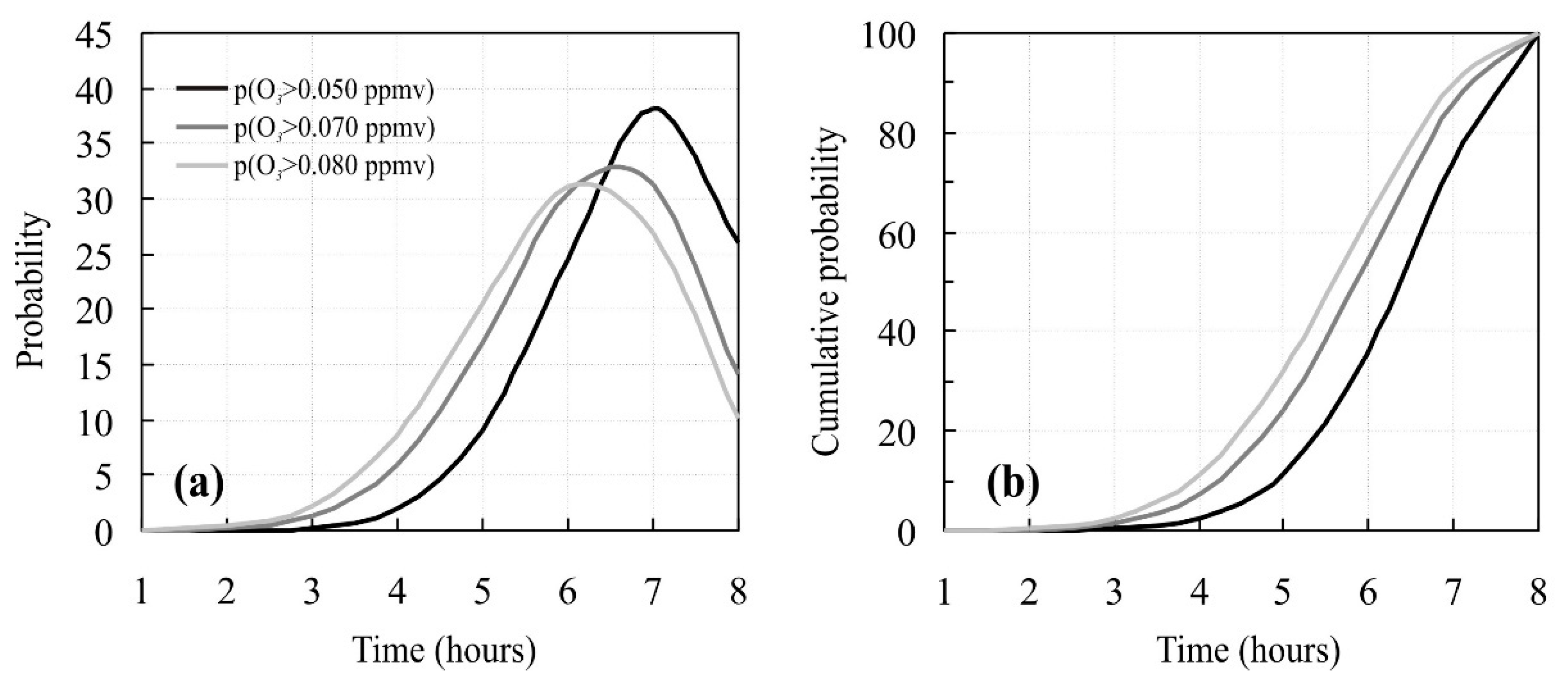
2.5. Statistical Probability

In addition to the analysis of the 1-h and 8-h moving average values, the statistical probability based on a binomial function (Equation (2)) was used to evaluate the probability that ozone exceeds three different maximum permissible limits (0.080, 0.070, and 0.050 ppmv) in the different temporal window during the day. Together with the NDO3I, they show the high ozone concentrations over the entire study period and how they may be over short periods (hours). This function helps us to understand the frequency of the ozone measurements above any MPL, in terms of their probability. The following propositions support the criteria to build the function: (1) any ozone observation such that the ozone concentration is a typical value, and (2) a fixed probability related to a specific limit such that the ozone above that limit is a successful event (poor air quality).
p ( x ) = ( n x ) · p x · q n x ,   ( n x ) = n ! x ! ( n x ) !  
where p is the probability of success, q is the probability of failure, x is the variable that measures the success in n number of hours, and n is defined here as an 8-h temporal window. The last constant takes into account that the tropospheric ozone is directly related to the intensity of natural light. Since the highest concentrations commonly occur along with the temporal windows from ten to twelve hours a day (approximately 7 a.m. to 7 p.m.) with some variations associated with seasonal changes. The statistical, probabilistic approach takes a temporal window of eight hours as the possible period to find high ozone concentrations. This takes into account that the solar radiation becomes negligible in the early sunrise hours and the last sunset hours.

3. Results and Discussion

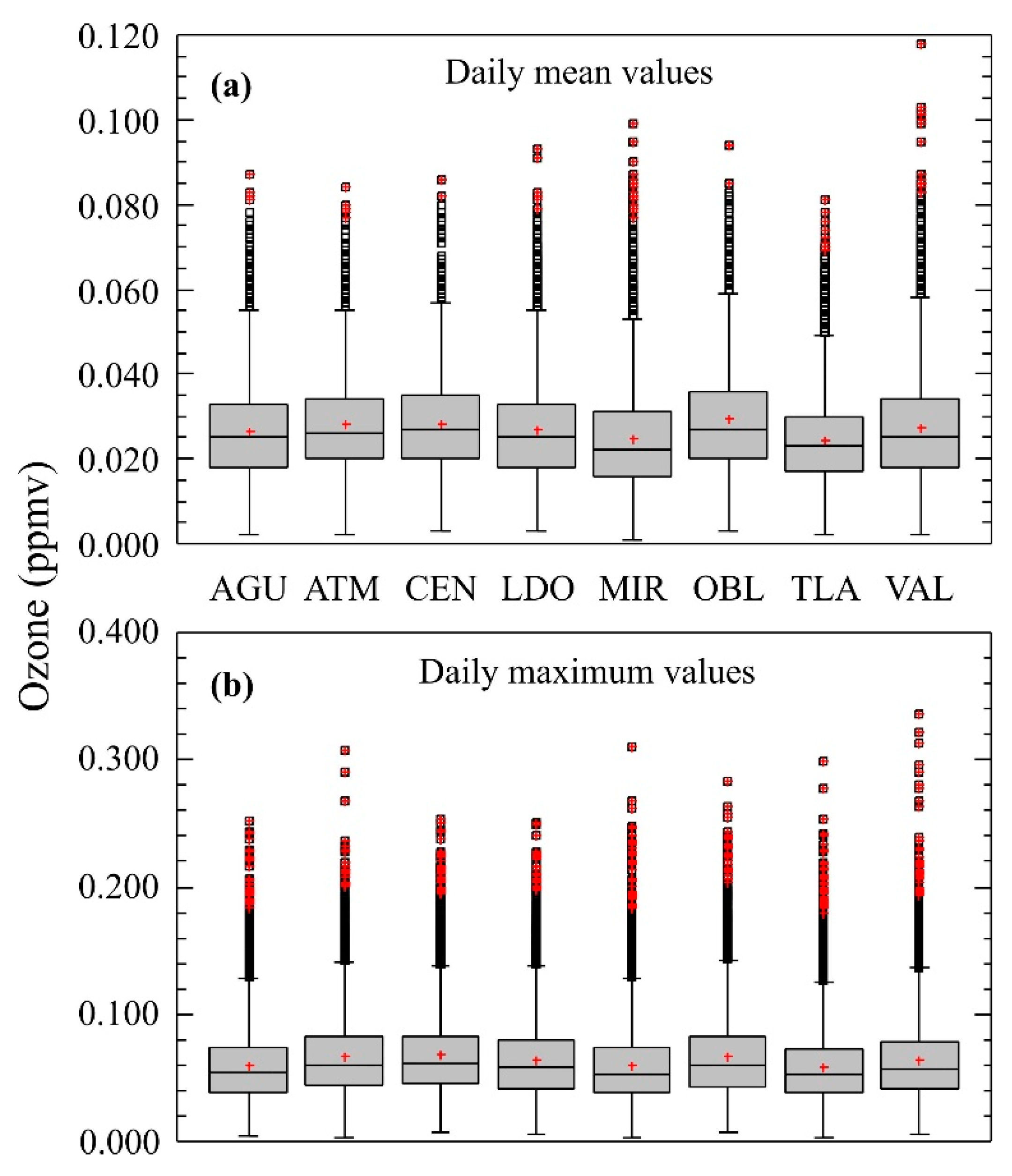
3.1. Spatial Variation

The comparison between stations showed that at least 50% of the ozone measures were close to the median values (Figure 3). The statistics indicate that the median values of all stations were in a short range of 0.022 to 0.027 ppmv for the daily mean ozone and 0.052 to 0.060 ppmv for the maximum ozone. The small differences among sites indicate that there are no important spatial gradients, helping to draw a quasi-homogeneous air pollution condition in the city. Such similarities comprehensively allowed us to characterize the ozone throughout the entire area of influence. In this sense, every parameter should be considered as the result of the eight stations, to interpret the average of the mean values (mean ozone), the maximum (maximum ozone), and the average of the maximums (maximum average); with the later statistical parameters measurable only from daily to smaller scales (e.g., monthly or yearly).

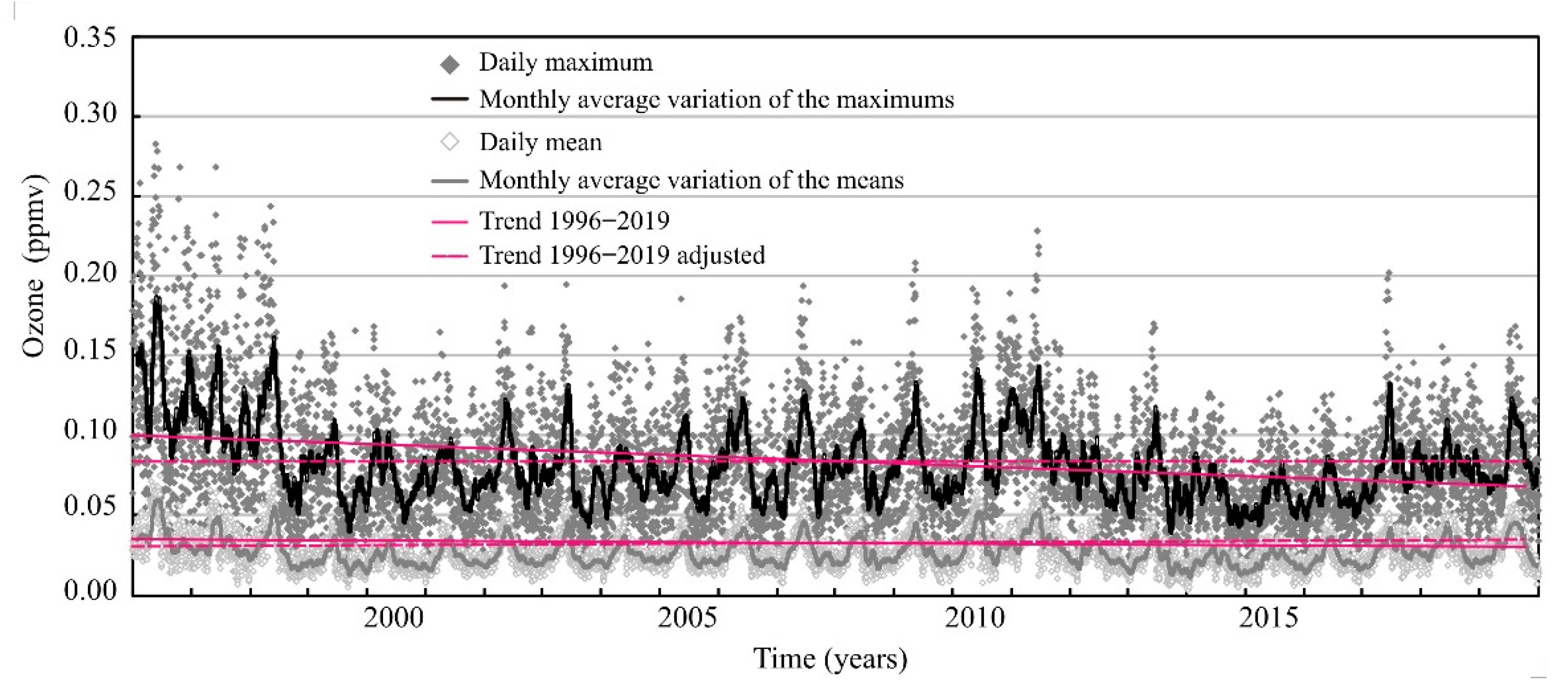
3.2. Long-Term Trend Analysis

3.2.1. Bias Trends

The time series analysis highlights important aspects of the tropospheric ozone in GMA. Two periods (1996–1998 and 2010–2011) were identified with atypical concentrations (Figure 4). A statistical comparison between monthly ozone showed that those atypical years, significantly, were 32.2 to 45.8% higher than the values in the typical years (p < 0.05) (Table 1). Their seasonal variation followed a normal pattern with high concentrations in the warm–dry season and lower concentrations during the rainy season, such as in all other years in the time series (Described in Section 3.3). However, the prominent contrasts with the previous or later years suggest possible systematic errors. Therefore, a comparative analysis identified their incidence in the long-term trend. The case considering all the twenty-four years delineated a decreasing trend over the full period, which is more evident for the maximum ozone. In contrast, the exclusion of the five atypical years shows a reasonable increase in the mean ozone trend, while the maximum ozone remains quasi-stable (Figure 4). These results represent an update of the ozone trends, considering the largest volume of data analyzed so far in the study area, in comparison with previous studies.

3.2.2. Atypical Ozone Measurements

The analysis of variance indicates that there are no significant differences, whether or not we consider these atypical years in the global assessment (p < 0.05, with an r2 = 0.98). These highly atypical values preserve compliance with annual ozone cycles and seasonal patterns; however, they induce a decrease in the long-term ozone trend at the end of the period, similarly to that reported in recent studies for shorter periods [20,21]. Such a trend is opposed to the growing number of mobile sources with an average annual growth rate of 3.5% in the last decade, or 4.2% in the last five years. Since vehicles are the main source of ozone precursors, the long-term trend of ozone could be determined. Therefore, its growth rate suggests similar increases of ozone precursors, and, eventually, a consequent increase of the ozone concentrations. On the other hand, systematic errors based on the technological adaptation of the monitoring system could also explain the evident decrease in the inter-annual trend observed between 1996 and 1998. The partial or total obsolescence of the measurement equipment that was not replaced could affect its optimal functioning, producing measurement deviations such as those observed from 2010 to 2011 [29]; deviations seem to be related to problems such as the calibration of the analyzers, adjustment of the calibration bands, and the ozone dilution standard (personal communication). Given these reasonable discrepancies with the mobile sources and probable systematic deviations, we excluded atypical periods from the analysis.

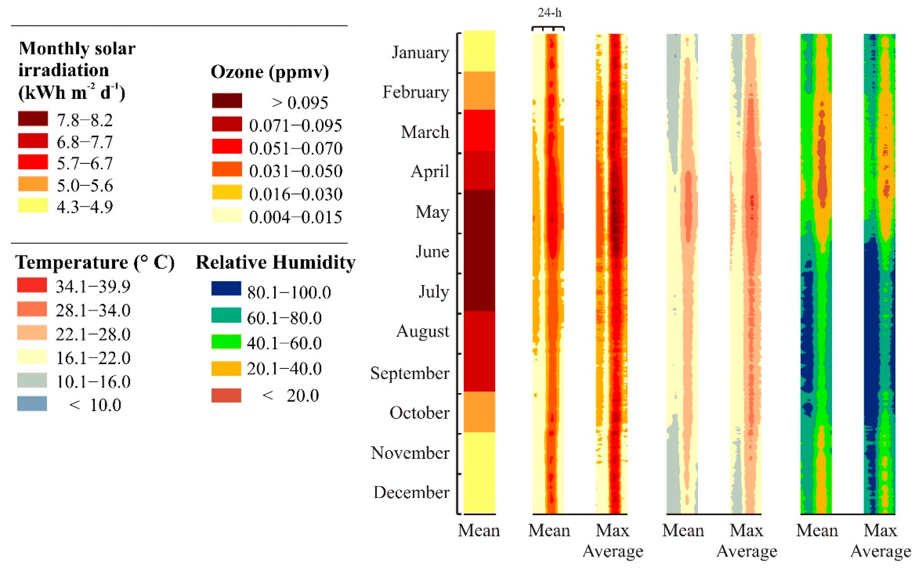
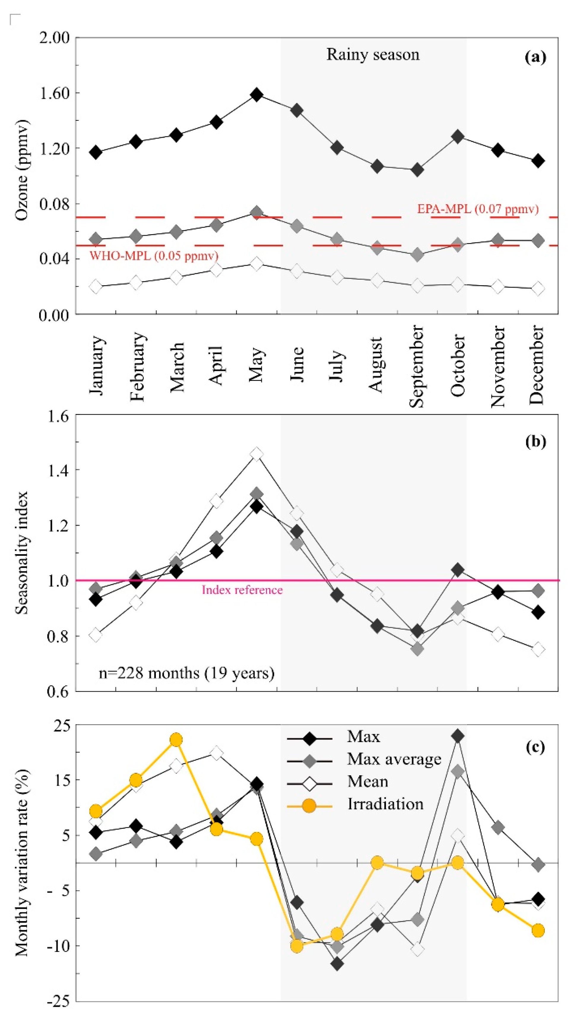
3.3. Inter-Annual Cycles and Seasonal Variability

3.3.1. Pattern Description

The inter-annual cycles followed a temporal pattern with regular and periodic variations, closely associated with a stable long-term trend. In this context, the evaluation of the seasonal variations was in terms of the monthly average values of the nineteen typical years. The mean ozone showed a clear seasonal pattern of high values during the spring–summer season (March–August) and low values in the summer to fall (September–February) in almost all years, remaining within concentrations below 0.040 ppmv (0.019−0.036 ppmv), a quantity relatively safe for public health (Figure 5a). Conversely, the maximum ozone showed high values in May and October, divided by the rainy season. Their concentrations were up to three times the mean ozone, reaching up to 0.159 ppmv in May, and with the lowest close to 0.100 ppmv in August and September. While the maximum average ozone become moderate, which varied in the range of 0.043 to 0.073 ppmv, with regular concentrations above the WHO and EPA-MPL almost all the year. This parameter shows the proper, but conservative, high ozone concentrations following the temporal pattern of the mean values.
The seasonal index explains the monthly variability throughout the course of the annual cycle. The mean ozone had main seasonal changes up to 70.5%, while, the maximum and averages of the maximum were 45 and 55.9%, respectively (Figure 5b). These results highlight the importance of the mean values in showing a remarkable stationary contrast. In addition, the seasonal index denotes that maximum ozone and its average values preserve the smaller annual seasonal change; emphasizing a semi-permanent state of high pollution throughout the inter-annual cycle, diminishing only in the second half of the rainy season.

3.3.2. Human and Environmental Influences

The GMA has a highly photo-reactive atmosphere, which may be related to the high amount of ozone and the chemical precursors derived from the vehicular fleet [30]. Solar irradiation becomes a determining factor that favors ozone formation. The monthly solar irradiation that potentially reaches the surface of the GMA is higher during the spring–summer seasons (Figure 2); however, the cloudy skies associated with the high atmospheric humidity tend to attenuate the irradiation during the rainy season [24]. Considering this seasonal pattern, the evaluation of solar irradiation helps in understanding its influence on the seasonal variation of ozone. A comparison of their changes, evaluated in terms of the monthly exchange rate, shows the direct dependence of the ozone as a response to the solar irradiation variation (Figure 5c). A prominent fall in the proportion of solar irradiation for the dry–warm to the rainy seasons and the persistently negative rate until September explains the temporal variations in the monthly ozone concentrations; mean ozone is better adjusted to such temporal patterns.
In this sense, the statistical analysis confirms that solar irradiation strongly correlates with the mean ozone (r = 0.93, p < 0.05), explaining 86% of its variance. While the correlation was moderate, with the maximum (r = 0.80, p < 0.05) and maximum average ozone (r = 0.77, p < 0.05) explaining the 64.3 and 58.9% of the variation, respectively. The correlation degree of the ozone formation, as a function of the solar radiation availability, denotes the importance of the cloudy sky conditions in the rainy season, which attenuates the formation rate of the tropospheric ozone. The statistical analysis also shows that the three statistical parameters of the ozone preserve significant differences among them (p < 0.05); this is a property that can be better observed if the information is analyzed at a diurnal temporal scale. These results show that solar radiation is a fundamental factor that drives the seasonal variation of ozone; however, its normal cycle could not generate variations in the long-term trend of ozone concentrations.
On the other hand, the old and unregulated automobiles of the GMA contribute to the increase of NOx, the inventory in the state shows that close to 70% of the vehicle fleet is composed of units produced before 2006 [31]. Statistical information published by the local environmental agency shows that NOx emissions have diminished over time [29]; the NOx trend corresponds with a slight decrease of the annual fuel consumption, which was close to 15% between 2011 and 2015, having a sharp decrease in 2016. These NOx emissions together with the VOCs, both induce a VOC-NOx sensitive regime that regulates the ozone formation [32]. This chemical regime and its causes could explain the semi-stable and even the slightly negative ozone trend. Therefore, permanent monitoring of VOCs could contribute to improving the understanding of the ozone regime and its main sources.

3.4. Diurnal Changes

The long-term analysis of monthly and seasonal ozone variation helped to understand the normal behavior over time. Moreover, the analysis of the mean and maximum concentrations above critical limits with the use of the NDO3I allowed us to highlight the magnitude and period in which the highest concentrations occur. The ozone index and the critical standard EPA [14] showed a common diurnal pattern along with the twenty-four-hour records, when the ozone exceeds this limit and remains above it for extended periods (Figure 6a,b). The mean ozone smooths the high values of the maximum of ozone at all of the monitoring stations, eventually, hiding ozone peaks above that limit. In the inter-annual cycle, the ozone intermittently exceeds the EPA limit, this can be seen in the first half of the year when high concentrations could reach up to eight hours or more. Instead, the ozone decreased below 0.070 ppmv in the rainy and fall–winter seasons.
A similar analysis of the critical WHO-MPL depicts high ozone concentrations from eight to sixteen hours during the spring–summer season (Figure 7a,b). Diurnal events were also very common during the fall–winter season, when NOx emissions increased due to changes in the atmospheric dynamics linked to the typical thermal inversion of the season [33]. The ozone increased in the rainy period, compared to the WHO limit, despite significant proportions of solar irradiation available at the ground level (23–28%) being attenuated by humidity and cloudy sky. The occurrence of sunny days throughout the rainy season explains the eventual high ozone concentrations, because of the photochemical reaction of the ozone precursors [24].
Comparison of the frequency between records above the USEPA standard and WHO guideline, as well as differences between the mean and maximum ozone showed evidence of the number of hours per day in every year during which the population in the GMA had been exposed to unhealthy ozone levels. The mean values seem to underestimate worrisome ozone concentrations, while, the maximum values overestimated such levels. In both cases, the parameters reflect extreme conditions that, far from helping to make a better decision, in the best of cases contribute to keeping environmental protection policies the same.

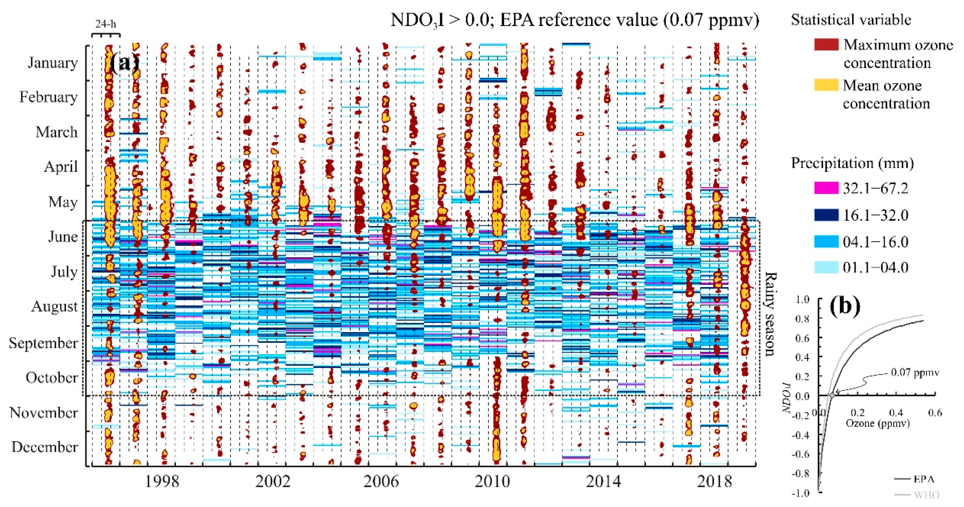
3.5. Tropospheric Ozone under the Strictest Limit

3.5.1. Comparison among Standards

The nineteen typical years depict important differences, depending on the MPL values and the three statistical parameters. A comparative analysis regarding 8-h moving average concentration based on the average maximum and average values of the maximums was obtained from the eight stations. A time series with more than 166 thousand hourly records showed the scenario of air pollution by ozone in the GMA. It is clear that, when lowering the MPL, a major number of hourly records could be classified as periods of poor air quality.
The Mexican standard establishes poor air quality for health protection under two different criteria, one similar to EPA’s criterion, and the other when the ozone concentration exceeds 0.095 ppmv in one hour at least once a year. Time series analysis, regarding the limit 0.095 ppmv, showed that about 0.4% of the hourly mean ozone did not meet this standard in any station; if such a standard is applied to the maximum values, 3.6% of the hourly measures would be above that limit (Table 2). The percentage of poor air quality events is apparently very small (0.4%); however, there are about 35 events per year on average when ozone concentrations are extremely high. In the best scenario, these high-risk events may contribute to an increase cases of breathing problems, such as inflammation, irritation, cough, and tightness in the chest.
The EPA and WHO MPLs for 8-h moving average concentrations were evaluated, taking into account the three parameters (Table 2). The analysis showed that 3.4 and 12.4% of the mean ozone, obtained from all records, were above the 0.070 and 0.050 ppmv, respectively, which could be classified as poor air quality. Furthermore, the frequency of poor air quality events increases dramatically, if we consider the maximum ozone concentrations, 10.8 and 23.7% for EPA and WHO MPLs, respectively. A similar proportion occurs with the maximum average ozone, the frequency of poor air quality events is close to 7.7 for EPA and 22.8% for WHO MPLs.
A comparison between mean ozone and EPA MPL (under the criterion of an 8-h moving average) showed that about 255 high ozone events per year were above such a limit, which means 0.7 events per day based on the mean ozone. While, the maximum average ozone measured in any place of the city showed that 588 high ozone events per year were above such a limit, which means 1.6 events per day. The same analysis, referred to the WHO MPL, indicated that the maximum average ozone was above 0.050 ppmv 1750 times per year (on average); which means 4.8 events per day over the two decades. This frequency is 6.8 times the frequency recorded with the mean ozone above the EPA MPL.
On the other hand, the probability function was estimated in eight-hour periods for the WHO’s guideline, EPA’s standard and the last Mexican standard (Table 3). The function showed that events with high ozone concentrations exceeding all MPLs for one to four hours tend to be small (up to 8.5%) (Figure 8a,b). The probability increases to between 20.4 to 38.1% for events with durations of five to seven hours; particularly, the probability that high concentrations will remain above the EPA and WHO-MPLs for seven hours is between 31.3 and 38.1%, respectively. While, the high-ozone events prevailing for up to eight hours above such MPLs range from 10.2 to 25.9% probability, respectively.
Measurements and statistical probability showed that high ozone concentrations remained for several hours a day. Normally, ozone does not remain for more than 8 consecutive hours; however, the WHO warns that exposure for periods of 5 to 7 h represents a risk to the population’s health [12,13]. These results show evidence for claiming the strictest MPLs, to establish the real context of the air pollution from ozone, highlighting the need to consider alternative statistical criteria in the air quality evaluation of ozone or other pollutants.

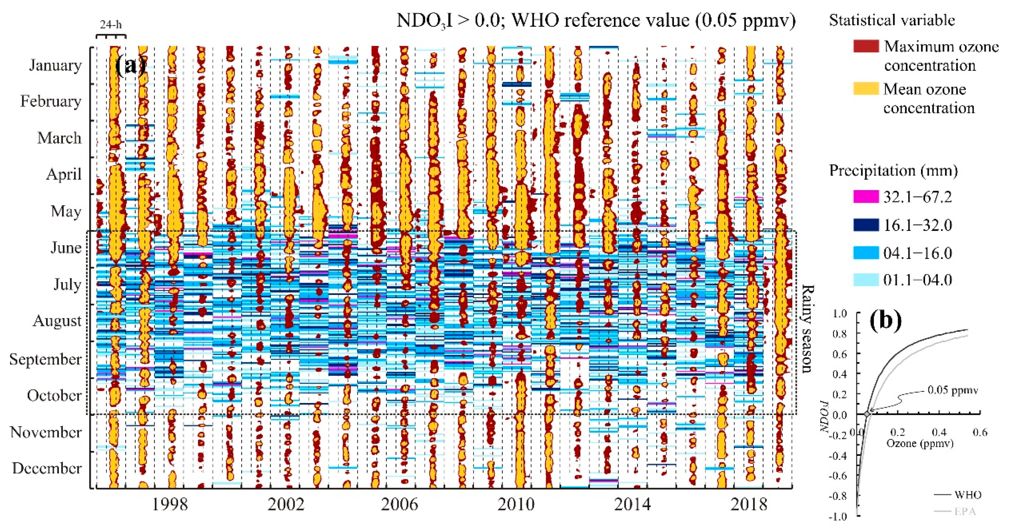
3.5.2. Normal Pattern under the WHO-MPL

The entire time series of an annual cycle was summarized to show the normal ozone variations under the WHO reference limit, considering the hourly records and the three statistical parameters in terms of the NDO3I values. The analysis shows that the ozone measurement is above the WHO standard and any MPL over the years. Mean ozone hardly reaches up to 10% of the time in exceeding the 0.05 ppmv in the entire cycle; maximum average values were close to 29%; while, maximum ozone exceeded 65% (Figure 9a). Such percentages reveal that the frequency of high ozone concentrations, concerning the WHO limit, persisted for approximately a third of the time in the GMA.
Furthermore, the NDO3I delineated the normal temporal boundary between high ozone concentrations (above WHO-MPL) and those with the least risk to public health (Figure 9b). Special attention should be given to the maximum average ozone, which typically tends to be above the 0.050 ppmv, close to the solar noon and for six or more hours, almost all the year. Meanwhile, the mean and maximum parameters seem to be far away from explaining the typical high ozone concentrations; this is due to the mean underestimating the highest ozone concentrations, while the maximum represents the extremely high concentrations observed all the time. The hourly time series and probabilistic approach show that the maximum average ozone concentrations depict a better correspondence with the more realistic levels of the tropospheric ozone pollution observed in the GMA, all in the context of the WHO guidelines.
In the light of these results, it is questionable whether the MPLs based on current parameters prevent damage to health. This is taking into account that high ozone concentrations for periods of six to eight hours per day could be sufficient to produce adverse health effects in the short term for susceptible groups of the population [12]. Furthermore, long-term exposition could be the cause of many lung disease cases and mortality in the GMA. The results from this research point out the potential advantages of taking into account the maximum average ozone as an additional criterion, to prevent these kinds of effects on public health.

3.6. Implications

The air quality regulation appears to be underestimated, in light of international conventions. Since relatively low ozone concentrations have been considered harmful to public health in urban areas [15], more restrictive pollution control policies are required to ensure better air quality in urban areas. Air pollution by ozone is an issue that must be addressed with the greatest responsibility, to reduce its effects on public health. A few countries, such as India, have adopted the strictest ozone limit (0.050 ppmv) [34]. Whereas, Brazil, United States, and Mexico have tightened their maximum permissible limits to levels of 0.070 ppmv [14,18,35]; while, European Union members and Canada and Japan, have preserved a limit of 0.060 ppmv [36,37,38].
Adoption of WHO-guidelines for ozone represents a great challenge, due to the vehicular fleet and industrial activities typically growing, and consequently, ozone precursors are increasing in urban areas. The actions derived from such guidelines should be accompanied by other measures to regulate the ozone precursors and improve the air quality in urban areas. This study leads us to raise the requirement to review the current criteria for controlling air pollution. The assessment of high ozone levels based on public information provides a complementary perspective to develop better schemes of prevention, contributing to more documented decision-making. The results obtained here suggest that the average of the maximum values could be adapted as a complementary reference to estimate the probability of exceeding any MPLs in the immediately following years. The adoption of this parameter will help to establish a baseline for assessing air quality under seasonal variability or trends in the short- and medium-term.
The use of maximum average values intended as an auxiliary criterion could reinforce decisions in the current programs of state environmental contingencies for health protection regarding the ozone or other criteria pollutants such as NOx. Important public resources for health care could be saved because of the reduction in the number of medical consultations for ozone-related diseases. Additionally, the strictest limit would also demand and promote improvements in several sectors, such as (1) alternative energy development; (2) new agreements and policies to reduce emissions from mobile sources into the atmosphere, such as the transition from combustion engine vehicles to hybrid or electric vehicles; (3) technological solutions to control the precursors (VOCs and NOx); (4) the updating of environmental politics to establish stricter criteria to the atmospheric contingencies declarations, including regulation of ozone precursors; and (5) the update of instruments and components or the system of renovation for optimized and reliable monitoring systems, including the VOCs, among others.
Ozone is a secondary pollutant that strongly depends on its precursors, such as VOCs and NOx; nevertheless, their regulation is a serious and common problem that faces many governments for air pollution evaluation. In Mexico, this is not different, and NOx information is available; however, the national monitoring network does not measure the VOCs systematically. Therefore, it is necessary to find a new alternative source to solve the gap in the VOCs information and reach an understanding of the mechanisms behind the ozone rate and its sensitivity to precursors. In this sense, the results derived from the present study could help to underline the need to consider their inclusion in permanent monitoring programs.

4. Conclusions

This study indicates that it may be necessary to consider the maximum average ozone as a complementary parameter, to decrease human health risks in urban areas. Our results indicate that the maximum ozone and the maximum average ozone showed important temporal patterns that are hard to see only with the mean ozone. Among the most important findings is the persistence of high values above the WHO limits for long periods throughout the day, which are highly frequent over the annual cycle. The implementation of these measures could be replicated and evaluated by the scientific community, to be discussed in the international agenda, and eventually adapted by convention in most countries.

Author Contributions

Conceptualization, J.d.J.D.-T.; methodology, J.d.J.D.-T. and M.A.M.-T.; validation, H.A.S.-N. and J.V.-S.; formal analysis, J.d.J.D.-T., V.O.-C., L.H.-M. and M.A.M.-T.; investigation, J.d.J.D.-T.; data curation, J.d.J.D.-T.; writing—original draft preparation, J.d.J.D.-T.; writing—review and editing, J.d.J.D.-T., M.A.M.-T., H.A.S.-N. and J.V.-S.; visualization, J.d.J.D.-T. and M.A.M.-T.; supervision, J.d.J.D.-T. and M.A.M.-T.; project administration, L.H.-M.; funding acquisition, M.A.M.-T., L.H.-M. and J.d.J.D.-T. All authors have read and agreed to the published version of the manuscript.

Funding

This work was supported by the National Council of Science and Technology in Mexico (CB-2012/183444).

Institutional Review Board Statement

Not applicable.

Informed Consent Statement

Not applicable.

Data Availability Statement

The datasets generated during and/or analyzed during the current study are available from the corresponding author on reasonable request.

Acknowledgments

We would like to thank the Ministry of Environment in the State of Jalisco for the availability of air pollutants and meteorological data. Particularly to Estefany López as Air Quality Management Director and the engineer Jorge Blanco as Coordinator of the State Monitoring Network.

Conflicts of Interest

The authors declare no conflict of interest.

References

  1. WHO. Fact Sheet: Ambient (Outdoor) Air Pollution. Available online: https://www.who.int/news-room/fact-sheets/detail/ambient-(outdoor)-air-quality-and-health (accessed on 30 June 2021).
  2. Malley, C.S.; Henze, D.K.; Kuylenstierna, J.C.; Vallack, H.W.; Davila, Y.; Anenberg, S.C.; Turner, M.C.; Ashmore, M.R. Updated global estimates of respiratory mortality in adults≥ 30 years of age attributable to long-term ozone exposure. Environ. Health Perspect. 2017, 125, 087021. [Google Scholar] [CrossRef] [PubMed] [Green Version]
  3. Finlayson-Pitts, B.J.; Pitts, J.N., Jr. Chemistry of the Upper and Lower Atmosphere: Theory, Experiments, and Applications; Academic Press: San Diego, CA, USA, 2000. [Google Scholar]
  4. Eiguren-Fernandez, A.; Miguel, A.H.; Lu, R.; Purvis, K.; Grant, B.; Mayo, P.; Di Stefano, E.; Cho, A.K.; Froines, J. Atmospheric formation of 9,10-phenanthraquinone in the Los Angeles air basin. Atmos. Environ. 2008, 42, 2312–2319. [Google Scholar] [CrossRef]
  5. Zhang, L.; Jacob, D.J.; Boersma, K.F.; Jaffe, D.A.; Olson, J.R.; Bowman, K.W.; Worden, J.R.; Thomson, A.M.; Avery, M.A.; Cohen, R.C.; et al. Transpacific transport of ozone pollution and the effect of recent Asian emission increases on air quality in North America: An integrated analysis using satellite, aircraft, ozone-sonde, and surface observations. Atmos. Chem. Phys. Discuss. 2008, 8, 8143–8191. [Google Scholar] [CrossRef] [Green Version]
  6. Walgraeve, C.; Demeestere, K.; Dewulf, J.; Zimmermann, R.; Van Langenhove, H. Oxygenated polycyclic aromatic hydrocarbons in atmospheric particulate matter: Molecular characterization and occurrence. Atmos. Environ. 2010, 44, 1831–1846. [Google Scholar] [CrossRef]
  7. Haagen-Smit, A.J. Chemistry and physiology of Los Angeles smog. Ind. Eng. Chem. 1952, 44, 1342–1346. [Google Scholar] [CrossRef]
  8. Wild, O.; Akimoto, H. Intercontinental transport of ozone and its precursors in a three-dimensional global CTM. J. Geophys. Res. Atmos. 2001, 106, 27729–27744. [Google Scholar] [CrossRef] [Green Version]
  9. Molina, L.; Molina, M.J. Air Quality in the Mexico Megacity: An Integrated Assessment (Vol. 2); Kluwer Academic Publishers: Dortrecht, The Netherlands, 2002; 384p. [Google Scholar]
  10. Akimoto, H. Global air quality and pollution. Science 2003, 302, 1716–1719. [Google Scholar] [CrossRef] [PubMed] [Green Version]
  11. Kopacz, M.; Jacob, D.J.; Fisher, J.A.; Logan, J.A.; Zhang, L.; Megretskaia, I.A.; Yantosca, R.M.; Singh, K.; Henze, D.K.; Burrows, J.P.; et al. Global estimates of CO sources with high resolution by adjoint inversion of multiple satellite datasets (MOPITT, AIRS, SCIAMACHY, TES). Atmos. Chem. Phys. 2010, 10, 855–876. [Google Scholar] [CrossRef] [Green Version]
  12. WHO. Air Quality Guidelines for Europe, 2nd ed.; European Series, No. 91; WHO Regional Publications: Copenhagen, Denmark, 2000; 288p. [Google Scholar]
  13. WHO. Health Aspects of Air Pollution: Results from the WHO Project "Systematic Review of Health Aspects of Air Pollution in Europe"; (No. EUR/04/5046026); WHO Regional Office for Europe: Copenhagen, Denmark, 2004. [Google Scholar]
  14. USEPA (United States Environmental Protection Agency). National Ambient Air Quality Standards for Ozone, Rules and Regulations; Federal Register; US Government: Washington, DC, USA, 2015; Volume 80, No. 206; 177p.
  15. WHO. WHO Air Quality Guidelines for Particulate Matter, Ozone, Nitrogen Dioxide and Sulfur Dioxide: Global Update 2005: Summary of Risk Assessment; (No. WHO/SDE/PHE/OEH/06.02); World Health Organization: Geneva, Switzerland, 2006; 22p. [Google Scholar]
  16. Bell, M.; Peng, R.D.; Dominici, F. The Exposure–Response Curve for Ozone and Risk of Mortality and the Adequacy of Current Ozone Regulations. Env. Health Perspect. 2006, 114, 532–536. [Google Scholar] [CrossRef] [PubMed] [Green Version]
  17. SEMADET. Air Quality Reports of the Guadalajara Metropolitan Area, 1996–2019. Available online: http://siga.jalisco.gob.mx/aire2020/reportes2020 (accessed on 30 June 2021).
  18. Health Secretary. Official Mexican Standard NOM-020-SSA1-2014, Environmental Health. Allowable Limit Value for the Concentration of Ozone (O3) in Ambient Air and Criteria for Its Evaluation. Mexican Official Diary. 2014. Available online: dof.gob.mx/nota_detalle.php?codigo=5356801&fecha=19/08/2014 (accessed on 8 January 2022).
  19. Benitez-Garcia, S.E.; Kanda, I.; Wakamatsu, S.; Okazaki, Y.; Kawano, M. Analysis of criteria air pollutant trends in three Mexican metropolitan areas. Atmosphere 2014, 5, 806–829. [Google Scholar] [CrossRef] [Green Version]
  20. Hernández-Paniagua, I.Y.; Clemitshaw, K.C.; Mendoza, A. Observed trends in tropospheric O3 in Monterrey, Mexico, during 1993–2014: Comparison with Mexico City and Guadalajara. Atmos. Chem. Phys. 2017, 17, 9163. [Google Scholar] [CrossRef] [Green Version]
  21. Fonseca-Hernández, M.; Tereshchenko, I.; Mayor, Y.; Figueroa-Montaño, A.; Cuesta-Santos, O.; Monzón, C. Atmospheric Pollution by PM10 and O3 in the Guadalajara Metropolitan Area, Mexico. Atmosphere 2018, 9, 243. [Google Scholar] [CrossRef] [Green Version]
  22. Garcia, E. Modificaciones al Sistema de Clasificación Climática de Köppen; Instituto de Geografía, Universidad Nacional Autónoma de México: Mexico City, Mexico, 1988. [Google Scholar]
  23. Servicio Meteorológico Nacional. Available online: Smn.conagua.gob.mx/es/ (accessed on 8 January 2022).
  24. Díaz-Torres, J.J.; Hernández-Mena, L.; Murillo-Tovar, M.A.; León-Becerril, E.; López-López, A.; Suárez-Plascencia, C.; Aviña-Rodriguez, E.; Barradas-Gimate, A.; Ojeda-Castillo, V. Assessment of the modulation effect of rainfall on solar radiation availability at the Earth’s surface. Meteorol. Appl. 2017, 24, 180–190. [Google Scholar] [CrossRef] [Green Version]
  25. Ojeda-Castillo, V.; López-López, A.; Hernández-Mena, L.; Murillo-Tovar, M.A.; Díaz-Torres, J.D.J.; Hernández-Paniagua, I.Y.; Del Real-Olvera, J.; León-Becerril, E. Atmospheric distribution of PAHs and quinones in the gas and PM1 phases in the Guadalajara Metropolitan Area, Mexico: Sources and health risk. Atmosphere 2018, 9, 137. [Google Scholar] [CrossRef] [Green Version]
  26. Gobierno del Estado de Jalisco. Programa para el Mejoramiento de la Calidad del Aire en la ZMG 1997–2001; Gobierno del Estado de Jalisco: Guadalajara, Mexico, 1996; 219p. [Google Scholar]
  27. Zuk, M.; Tzintzun-Cervantes, M.G.; Rojas-Bracho, L. Tercer Almanaque de Datos y Tendencias de la Calidad del Aire en Nueve Ciudades Mexicanas, 1st ed.; Instituto Nacional de Ecología: Mexico City, Mexico, 2007. [Google Scholar]
  28. Statpoint, Inc. The User’s Guide to STATGRAPHICS® Centurion XV; Statgraphics Technologies, Inc.: The Plains, VA, USA, 2005; 287p. [Google Scholar]
  29. Gobierno del Estado de Jalisco. Programa para el Mejoramiento de la Calidad del Aire en la ZMG 2014–2020; Gobierno del Estado de Jalisco: Guadalajara, Mexico, 2013; 257p. [Google Scholar]
  30. SEMADET-Secretaria de Medio Ambiente y Desarrollo territorial. Inventario de Emisiones de Contaminantes Criterio del Estado de Jalisco; Gobierno del Estado de Jalisco: Guadalajara, Mexico, 2014; 97p. [Google Scholar]
  31. Gobierno del Estado de Jalisco. Informe Calidad del Aire 2016, Sistema de Monitoreo Atmosférico de Jalisco; Gobierno del Estado de Jalisco: Guadalajara, Mexico, 2017; 56p. [Google Scholar]
  32. Kanda, I.; Basaldud, R.; Magaña, M.; Retama, A.; Kubo, R.; Wakamatsu, S. Comparison of ozone production regimes between two Mexican cities: Guadalajara and Mexico City. Atmosphere 2016, 7, 91. [Google Scholar] [CrossRef] [Green Version]
  33. García, M.; Ulloa, H.; Ramírez, H.; Fuentes, M.; Arias, S.; Espinosa, M. Comportamiento de los vientos dominantes y su influencia en la contaminación atmosférica en la zona metropolitana de Guadalajara, Jalisco, México. Rev. Iberoam. Cienc. 2014, 1, 97–116. [Google Scholar]
  34. CPC–Central Pollution Control Board. National Air Quality Standards. Ministry of Environment, Forest and Climate Change; Govt. of India: New Deli, India, 2009.
  35. Barboza-Chiquetto, J.; Siqueira-Silva, M.E.; Cabral-Miranda, W.; Dutra-Ribeiro, F.N.; Ibarra-Espinosa, S.A.; Ynoue, R.Y. Air quality standards and extreme ozone events in the São Paulo megacity. Sustainability 2019, 11, 3725. [Google Scholar] [CrossRef] [Green Version]
  36. European Union. Directive 2008/50/EC of the European Parliament and of the Council of 21 May 2008 on ambient air quality and cleaner air for Europe. Off. J. Eur. Union 2008, 29, L152. [Google Scholar]
  37. CCME-Canadian Council of Ministers of the Environment. Guidance Document on Achievement Determination: Canadian Ambient Air Quality Standards for Particulate Matter and Ozone; Canadian Council of Ministers of the Environment: Winipeg, MB, Canada, 2012; 53p.
  38. MOE, Menister of the Environment, Government of Japan. Environmental Quality Standard in Japan for Air Quality; Menister of the Environment, Government of Japan: Tokyo, Japan, 2018.
Figure 1. Map with the monitoring network in the Guadalajara Metropolitan Area (GMA). Empty locator: stations excluded by incomplete information for the analyzed period. Abbreviations: Las Águilas, AGU; Atemajac, ATM; Centro, CEN; Loma Dorada, LDO; Las Pintas, LP; Miravalle, MIR; Tlaquepaque, TLA; Oblatos, OBL; Santa Fé, SF; Vallarta, VAL.
Atmosphere 13 00152 g001
Figure 2. Normal ozone concentrations and climatology of the temperature and humidity for the period of 1996 to 2019 compared with the monthly average potential solar irradiation. Adapted with permission from ref. [25]. Ojeda-Castillo et al., 2018.
Atmosphere 13 00152 g002
Figure 3. The statistical distribution of the daily ozone concentrations in the 8-stations in the monitoring network of the Guadalajara Metropolitan Area: (a) mean ozone, (b) maximum ozone. The box and whisker plot denote the lower quartile, median and upper quartile (box), the percentile 5 and 95 (whisker), mean (red asterisk), and outliers (black-red squares). Abbreviations: Las Águilas, AGU; Atemajac, ATM; Centro, CEN; Loma Dorada, LDO; Las Pintas, LP; Miravalle, MIR; Tlaquepaque, TLA; Oblatos, OBL; Santa Fé, SF; Vallarta, VAL.
Atmosphere 13 00152 g003
Figure 4. Time series sequences of the ozone in the Guadalajara Metropolitan Area.
Atmosphere 13 00152 g004
Figure 5. (a) Monthly ozone values regarding the maximum permissible limits of EPA standards and WHO guidelines, (b) Monthly ozone variation is based on the decomposition of the seasonal subseries and index of seasonality, and (c) comparison of the monthly variation between ozone concentrations and solar irradiation.
Atmosphere 13 00152 g005
Figure 6. (a) Ozone measurements above the EPA’s standard limit, derived from the ozone index (NDO3I) analysis of the twenty-four-years of the time-series sequence of the Guadalajara Metropolitan Area. (b) Graphical representation of the NDO3I referred to the EPA’s limit.
Atmosphere 13 00152 g006
Figure 7. (a) Ozone measurements above the WHO’s guidelines are expressed in terms of the ozone index (NDO3I) over twenty-four years in the Guadalajara Metropolitan Area. (b) Graphical representation of the NDO3I referred to the WHO’s limit.
Atmosphere 13 00152 g007
Figure 8. (a) The statistical probability of the ozone above some maximum permissible limits as a function of the number of hours for a given event. (b) Cumulative probability of the integrated temporal window.
Atmosphere 13 00152 g008
Figure 9. (a) Percentage of hourly ozone observed above the WHO guideline in terms of the NDO3I. (b) Normal variation over nineteen years of the hourly tropospheric ozone through the annual cycle given the three different statistical parameters. Abbreviation: normalized difference ozone index, NDO3I; maximum permissible limit, MPL.
Atmosphere 13 00152 g009
Table 1. Statistical comparison between typical and atypical periods of ozone concentrations.
Mean OzoneMax OzoneMax Average Ozone
MonthTypicalAtypicalDifference %TypicalAtypicalDifference %TypicalAtypicalDifference %
January0.0200.02839.10.1170.17751.30.0540.08048.4
February0.0230.03137.90.1250.19354.90.0560.07941.1
March0.0270.03529.70.1290.18845.20.0590.08238.2
April0.0320.03920.40.1390.19036.80.0640.08531.2
May0.0360.05243.90.1590.22843.50.0730.11354.7
June0.0310.04648.00.1470.22150.20.0640.09853.8
July0.0270.03116.90.1200.15730.00.0540.06520.9
August0.0240.03125.10.1070.14939.50.0480.06432.6
September0.0210.02624.80.1040.15346.30.0430.06039.4
October0.0220.02724.80.1280.19047.70.0500.06630.6
November0.0200.02734.10.1190.17648.40.0530.07845.4
December0.0190.02641.30.1110.17255.30.0530.08457.3
Average differences32.2 45.8 41.1
Typical concentrations correspond to monthly average values of the periods 1999–2009 and 2012–2019. Atypical to monthly average values of the periods 1996–1998 and 2010–2011. Ozone concentrations in ppmv.
Table 2. Ozone frequency analysis based on the typical dataset (19 years).
1-h Data8-h Moving Average Data
Total dataset166,560100.0%166,560100.0%
Filtred dataset155,13493.1%144,96787.0%
Mean ozoneFreq O3 > 0.095 ppmv (NOM) 16850.4%n.a.n.a.
Freq O3 > 0.070 ppmv (EPA) 2n.a.n.a.48703.4%
Freq O3 > 0.050 ppmv (WHO) 3n.a.n.a.17,74712.4%
Maximum average ozoneFreq O3 > 0.095 ppmv (NOM) 1n.a.n.a.n.a.n.a.
Freq O3 > 0.070 ppmv (EPA) 2n.a.n.a.11,1697.7%
Freq O3 > 0.050 ppmv (WHO) 3n.a.n.a.33,25922.8%
Maximum ozoneFreq O3 > 0.095 ppmv (NOM) 155913.6%n.a.n.a.
Freq O3 > 0.070 ppmv (EPA) 2n.a.n.a.15,64210.8%
Freq O3 > 0.050 ppmv (WHO) 3n.a.n.a.34,33323.7%
1 Mexican standard for permissible limit values; 2 EPA’s standard regulation for the air pollutants maximum permissible limits; 3 WHO’s Air Quality Guidelines; The filtered dataset implies the sufficiency criteria for quality and the subtraction of the statistical outliers. n.a. Not apply.
Table 3. Binomial function’s parameters.
Fixed Probability
Limits0.050 ppmv0.070 ppmv0.080 ppmv
p(O3 > limit)0.840.780.75
q(O3 > limit)0.160.220.25
n= 8 hO3 range = 0.003−0.322 ppmv
x= 1−8 h
Publisher’s Note: MDPI stays neutral with regard to jurisdictional claims in published maps and institutional affiliations.

