Article

Simulating the Effects of Land Surface Characteristics on Planetary Boundary Layer Parameters for a Modeled Landfalling Tropical Cyclone

Department of Geography, University of Florida, Gainesville, FL 32611, USA
*
Author to whom correspondence should be addressed.
Atmosphere 2022, 13(1), 138; https://doi.org/10.3390/atmos13010138
Submission received: 15 December 2021 / Revised: 7 January 2022 / Accepted: 9 January 2022 / Published: 14 January 2022
(This article belongs to the Special Issue Feature Papers in Atmosphere Science)

Abstract

:
This study examined whether varying moisture availability and roughness length for the land surface under a simulated Tropical Cyclone (TC) could affect its production of precipitation. The TC moved over the heterogeneous land surface of the southeastern U.S. in the control simulation, while the other simulations featured homogeneous land surfaces that were wet rough, wet smooth, dry rough, and dry smooth. Results suggest that the near-surface atmosphere was modified by the changes to the land surface, where the wet cases have higher latent and lower sensible heat flux values, and rough cases exhibit higher values of friction velocity. The analysis of areal-averaged rain rates and the area receiving low and high rain rates shows that simulations having a moist land surface produce higher rain rates and larger areas of low rain rates in the TC’s inner core. The dry and rough land surfaces produced a higher coverage of high rain rates in the outer regions. Key differences among the simulations happened as the TC core moved over land, while the outer rainbands produced more rain when moving over the coastline. These findings support the assertion that the modifications of the land surface can influence precipitation production within a landfalling TC.

1. Introduction

The warm core structures of tropical cyclones (TCs) are fueled by the latent heat flux from a warm sea surface. Although surface energy fluxes are key to TC genesis and intensification, researchers noted that evaporation occurring in the storm’s core cannot support the rain rates produced in the eyewall and outer rainbands [1]. The moisture that TCs utilize to produce copious amounts of precipitation mainly comes from the horizontal convergence of moisture within the planetary boundary layer (PBL) [2,3]. Much of this moisture is sourced from outside of the storm’s core. Rainfall production should increase with TC intensity due to the larger influx of moisture by the stronger low-level circulation as wind speed increases. During landfall, the decreased moisture availability and increased roughness length as air moves over the land surface are both unfavorable conditions which can reduce storm intensity and suppress rainfall. However, several researchers [4,5,6] have observed the intensification of TCs over a moist land surface.
Several studies have examined the effects of land surface conditions on TCs. A set of idealized studies [7,8,9] have shown that when a TC made landfall, the evaporation rate dropped dramatically because of the decreased moisture and increased roughness length over land. Therefore, the lower evaporation rate leads to a reduction in the latent heat fluxes required to fuel TCs. However, more recent studies have shown that with sufficient supply of latent energy, even with an increased surface roughness, a storm could still intensify over land [10,11,12,13,14]. Kimball’s [15] modeling study concluded that the increasing roughness length has a bigger impact on accelerating storm decay than decreasing moisture availability over land. Meanwhile, cases with more moisture over land can lead to substantially higher rainfall accumulations as the storm moves through the area.
Land surface conditions have important linkages to convection, cloud formation, and the production of precipitation. The existing literature has investigated the impact of several land surface characteristics on the PBL, such as surface roughness [16,17], soil moisture [18,19,20], albedo [21,22], land use and land cover change [23], and spatial heterogeneities [24]. Previous studies [7,8,9,15] suggest that of these characteristics, moisture availability and roughness length have the most influence on TC structure, which will be the focus of the current study.
Land surface energy and moisture budgets can be expressed as follows [20]:
RN=QG+H+L(E+T)
P=E+T+RO+I
where RN is the net radiative fluxes, QG is the soil heat flux, H is the sensible heat flux, L(E+T) is the latent heat fluxes, P represents precipitation, E is evaporation, T is transpiration, RO is run off, and I is infiltration. Equation (1) indicates that for the surface energy budget, net radiative fluxes depend on latent heat from evapotranspiration and turbulent sensible heat flux. Meanwhile, Equation (2) illustrates that precipitation is dependent on the evapotranspiration rates, which are dependent on the moisture content of the surface, when the other two variables are unchanged. Thus, changing the properties of the land surface to increase or decrease latent heat exchange affects both the energy and moisture budgets.
Sensible and latent heat values are strikingly different between bare soil and fully vegetated surfaces, and modeling studies have investigated how the PBL differs above these contrasting surfaces. Densely vegetated surfaces with moist soils can act as a catalyst in the hydrological cycle, creating positive feedback and enhancing precipitation recycling due to enhanced moisture availability [23,25]. The results of a study that replaced dry cropland with irrigated cropland in the lower Mississippi River alluvial valley show that increases in moisture availability led to decreases in sensible and increases in latent heat fluxes, with decreases in surface temperature and increases in dew point [26]. Moreover, heat fluxes are also highly correlated with the drag coefficient which is positively related to roughness length [27,28]. In this sense, with unchanged atmospheric conditions, the two major properties of land surface, roughness length (mainly determined by vegetation type), and moisture availability (determined by both vegetation and soil type) can significantly change the surface energy and moisture budgets by altering the fluxes of heat, moisture, and momentum within the PBL, which will influence precipitation [29,30].
Several previous studies excluded synoptic-scale forcing when examining the relationship between land surface conditions and cumulus activities [24,26,31,32]. However, a few studies have evaluated how the land surface conditions can affect PBL conditions under synoptic-scale forcing. Yang et al. [33] examined the sensitivity of the rainfall distribution in a synoptic storm system over an urban area and concluded that even under conditions of strong large-scale forcing, urbanization, which decreases land surface moisture and increases roughness length, can still alter the local distribution of heavy rainfall. A sensitivity study of atmospheric response to roughness length examined three frontal events and found that stronger events were associated with smaller, yet still detectable, deviations in latent/sensible heat fluxes and PBL height caused by changing roughness length [17]. Thus, even under synoptic-scale forcing, changes in land surface conditions could induce differences in boundary layer energy fluxes and precipitation production.
Most previous studies that explored the relationship between land surface conditions and TC structures utilized idealized simulations, which means that the model configuration contained numerous simplifications. These simplifications included but were not limited to a fixed land surface temperature, approximation of the Coriolis parameter, and the exclusion of a steering flow [7,8,9,14]. One notable exception is [15], which included a relatively weak steering flow, variable Coriolis parameter, and time-evolving land surface temperature. However, other factors, which had been previously shown to influence TC structure, such as the shape of the coastline [34], and the time of day that landfall occurs [35,36], realistic steering flow [37,38,39], realistic terrain [40], and non-prescribed sea surface temperatures (SSTs) [41,42] were not included in these cases. As a result, it is still unclear how land surface characteristics can influence the structure of TCs in a realistic setting that includes all of the factors mentioned above.
Hence, the goal of this study is to determine whether changing the land surface characteristics (i.e., roughness length and moisture availability) produces detectable changes in properties related to cumulus activities in the PBL and rainfall production in a landfalling TC. We utilize the Weather Research and Forecasting (WRF) model to perform multiple simulations of a TC that made landfall over Florida and South Carolina with realistic atmospheric and oceanic conditions over a modified land surface. After performing a control simulation with the actual land surface properties, four additional simulations are performed with homogeneous land cover and soil type representing high and low roughness length and high and low moisture availability. Before investigating changes to the PBL, we compare track, translation speed, intensity, and size among the simulations and to observational records of Atlantic basin TCs to ensure that the simulated outputs are realistic. To verify that our modifications to the land surface made the expected changes to the PBL, we examine conditions before the outer edge of the TC reaches the study area. We then examine the PBL conditions while the TCs pass over the study region. Finally, we measure differences in the precipitation hourly rates to relate the alteration of the PBL to rainfall production within the TC.

2. Materials and Methods

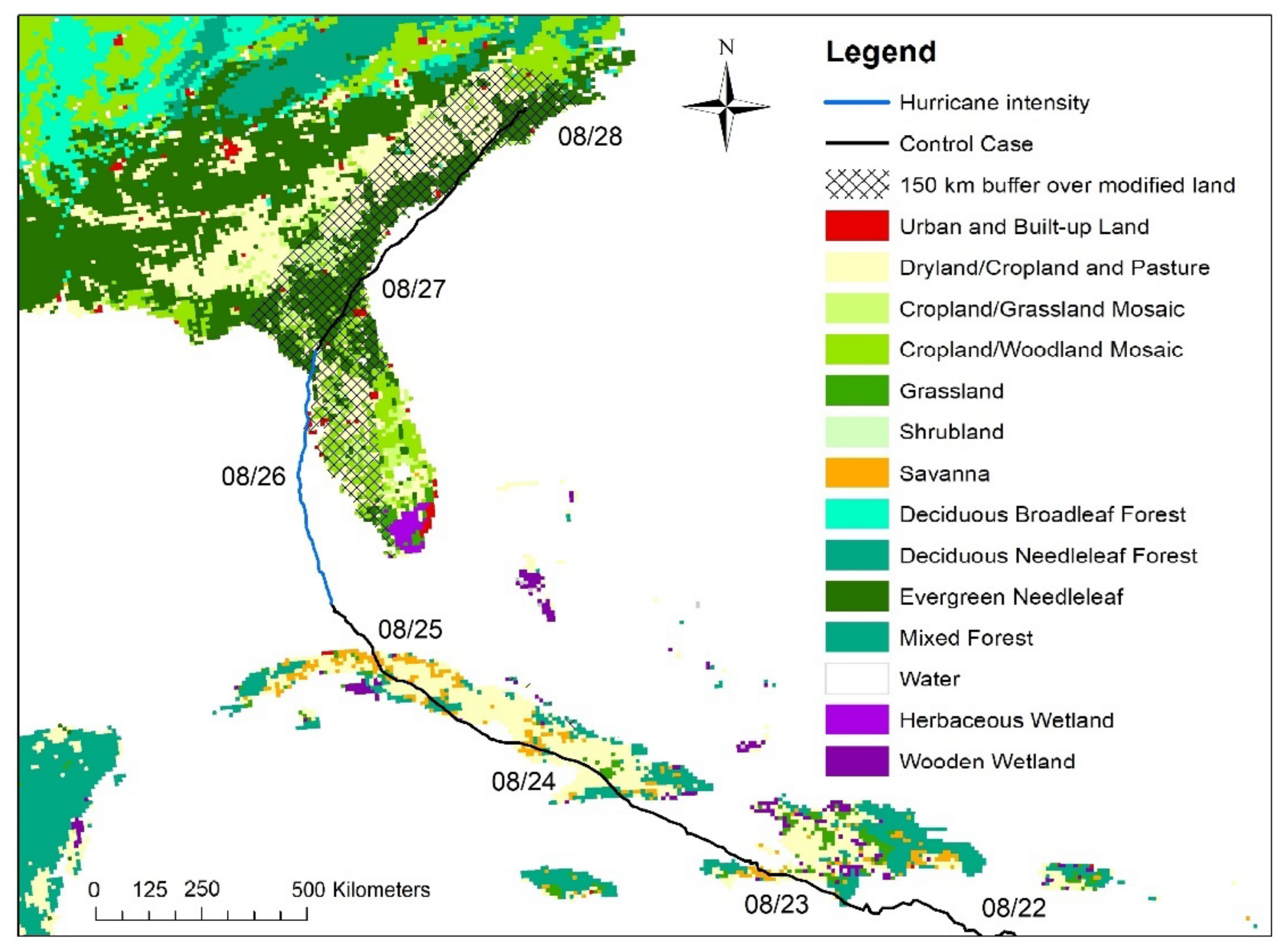
2.1. Nature Run and Case Selection

A “nature run” is a component of an observing system simulation experiment (OSSE), which is mainly used to generate simulated meteorological observations that can be input into weather forecast models, such as WRF, to assess the potential impact of additional observations, new observing systems, or new data assimilation schemes to improve numerical weather forecasts. A global nature run previously generated by the European Center for Medium range Weather Forecasting (ECMWF) used a free-running simulation with seasonal forcing and prescribed surface boundary conditions for 13 months over 2005–2006 [43,44], which is called the Joint OSSE Nature Run (JONR). After this simulation, [45] and [46] downscaled two TCs from JONR, using WRF 3.1.1 and 3.4.1 accordingly, and called them the hurricane nature run 1 and 2 (HNR1 and HNR2). The HNR2 made landfalls over Hispaniola, Cuba, and the southeast United States (Figure 1), which is used in this study. HNR2 has three nested domains, where the 1st domain is fixed and the 2nd and 3rd domains are vortex-tracking moving nests. The temporal resolutions are 30-min, 30-min, and 5-min, and domains consist of 480 × 360, 360 × 360, and 480 × 480 grid cells, respectively. The grid spacing of the HNR2 is 9 km, 3 km, and 1 km. In the situation of HNR2, the coastlines, topography, and land-use fields are well represented at 9 km.
The simulation period of HNR2 is from 1200 UTC 20 August to 1200 UTC 28 August 2005. The TC starts as a tropical wave over the northeast Caribbean Sea and makes its first landfall over Hispaniola. The storm moves further west and intensifies between Haiti and Cuba into a tropical storm at approximately 0600 UTC 23 August. Its second landfall occurs over Cuba as a tropical storm and then it turns towards the northeast. The warm waters of the Gulf of Mexico and low vertical wind shear contribute to the intensification of this TC to a Category 2 hurricane with a maximum sustained wind speed of 44 m s−1 at 1200 UTC 25 August. It makes its third landfall over the western coast of Florida near Tampa as a Category 1 hurricane. The time of landfall is 0600 UTC 26 August, and the maximum sustained wind speed is 34 m s−1. However, the center moves quickly back to water and a second Florida landfall occurs six hours later at Cedar Key. Even though there are two consecutive landfalls, we use the first landfall to compare with other cases as the eyewall continues to interact with the land surface between these two landfalls. Due to the land surface interaction, the storm quickly drops below hurricane intensity around 1200 UTC 26 August, moves northeast, and makes its fifth landfall around 1200 UTC 27 August over South Carolina as a tropical storm. This study focuses on the Florida and the South Carolina landfalls since at least half of the storm moves over land in both locations.
The TC in the Control case moves over several land cover types during its life (Figure 1). Many studies employ a 500 km radius from the storm center to define the outer boundary of a TC [47,48,49] and use the 100–150 km radius to define the inner core [50,51]. In this study, we use a distance of 500 km to define the outer edge of the storm. In the meantime, 150 km is used to distinguish the inner core from the outer region because HNR2 has a slightly larger eye (50 km) than found in the climatological study of Atlantic Basin TCs by [52]. The average roughness length is approximately 32.3 cm for the area within a 500 km radius and 30.2 cm within a 150 km radius. As roughness lengths can be >200 cm in a city center with high-rise buildings, yet be 0.02 cm over open water, this is a relatively smooth surface. As for soil moisture, the major soil type within both radii is loamy sand (more than 90%), which has a moisture availability of about 42%. This is a relatively high value considering that peat has 50% while coarse sand has 5% total available water.

2.2. Model Description and Experiment Design

In this research, the Weather Research and Forecasting–Advanced Research WRF 3.4.1 (WRF–ARW 3.4.1) is used to simulate the TC. This is the same model used to simulate the original HNR2 with the modification to surface layer drag coefficient based on WRF 3.1.1 by [46]. In our study, as in [46], a series of eight-day simulations is conducted with the outermost domain resolution of 9 km, and two vortex-tracking moving nests are set up with 3 km and 1 km grid spacing. All domains are initialized at 1200 UTC 20 August and end 8 days later at 1200 UTC 28 August. The global model JONR provides the initial and boundary conditions. A two-way interaction occurs between domains. There are 60 vertical levels, with the top pressure of 50 mb. WRF 6-class double-moment microphysics [53] is used as the microphysics scheme. For the radiation physics, RRTM-G shortwave and longwave radiation [54] is used. Additionally, the Kain-Fritsch cumulus scheme [55,56] is used on the outer grid (domain 1 only), the YSU planetary boundary layer scheme [57,58] is employed, and the Noah land surface model [59] is deployed on all domains. The physics and parameterizations we use are identical from the original HNR2 [46], where multiple schemes were tested and the current combination had shown to be the optimal choice. Moreover, a “nudging” process of large-scale fields to the global model is opened on domain 1 (9 km) with a specified 24-h time scale, to adjust the WRF model fields of horizontal velocity, temperature, and humidity for each 24-h time period [46]. We primarily report results from domain 2 (3 km), which has a better spatial resolution than domain 1, and the cumulus processes are not parameterized. The conditions occurring prior to the storm’s arrival are taken from domain 1 as domain 2 is centered on the storm and does not cover Florida prior to 0000 UTC 25 August. Meanwhile, domain 3 is opened to better resolve the core structure, but since its extent does not cover the whole storm, we do not report results from this domain.
After running the simulation with the actual land surface, we conduct four experiments based on the WRF set-ups described above. The land surface of the entire United States is modified to a homogeneous setup featuring one vegetation type and one soil type. This is realized by modifying the major vegetation and soil type in the input files of domain 1. Noting that the topography is not changed for all simulations, the averaged elevation within the 150 km buffer of the storm track is around 30 m. The WRF Land Surface Model defines the roughness length and moisture availability respectively according to the soil and vegetation type that are defined. We use two vegetation types, wetland and broadleaf forest, which have roughness lengths of 15 cm and 50 cm, respectively. Wetland and broadleaf are chosen because other than the dramatic difference they have in roughness lengths, all other parameters that can influence the near-surface atmosphere, such as leaf area index, albedo, emission, etc. are quite similar. We include two soil types of bedrock and water to represent moisture availability with 0% and 100%. Table 1 shows how roughness length and moisture availability varied among the four cases to produce conditions of Dry Smooth (DS), Wet Smooth (WS), Dry Rough (DR), and Wet Rough (WR).

2.3. Model Output Verification and Variables Comparison

The test cases are compared with the Control case first to ensure that key storm properties (track, intensity, and size) are similar to one another, and all cases are compared to actual TCs in the Atlantic Basin. The storm track is calculated based on the location of the minimum central pressure at the surface every 30-min. Distances from each case to the Control case are computed at each timestep and evaluated through the calculation of RMSE for the whole time series. Landfall locations and times are also compared. The intensities are evaluated by calculating RMSE relative to the Control case using both minimum central pressure at the surface and maximum sustained wind speed at 10 m. We also compare the translation speed among all simulations Next, storm size is represented by the radius of gale-force winds (17.5 m s−1), damaging force winds (25.7 m s−1), hurricane-force winds (32.9 m s−1), and maximum winds and outmost closed isobar (1007 mb), which are calculated and compared with [52]’s study of the sizes of Atlantic Basin TCs. Lastly, the environmental moisture profile, which is represented by total precipitable water (TPW) (direct outputs from the WRF model), defined as the total depth of water in a column of the atmosphere, is examined. Total precipitable water is examined to ensure the synoptic environments are consistent for all simulations, so that any differences in precipitation would not be due to variations in moisture above the PBL. Though changes are made in land surface characteristics, we still expect a realistic TC structure that is comparable with actual Atlantic Basin hurricanes as the TC spins up 3000 km away from the modified land surface.
To investigate the contribution of different land surface characteristics to the PBL, variations in three PBL variables related to precipitation production are examined before and during interaction with the storm. Time series of latent heat flux (LHF), sensible heat flux (SHF), and friction velocity (FV) near the surface, which are three variables directly available from the WRF output, are calculated by averaging values over land within the 150 km of the TC track for the periods before and during interaction with the storm. The periods are separated by the time that the radius of gale-force winds started to interact with U.S. mainland (around 0000 UTC 25 August). Data available every 30 min are examined 0000 UTC 22 August to 2300 UTC 24 August, which is prior to the storm’s interaction with the land surface. We refer to this period as time before storm (TBS). The three-day period when the storm is interacting with the land surface from 0000 UTC 25 August to 2300 UTC 27 August is termed time during storm (TDS). Figure 2 shows the region where the storm center is located during these two periods.
As changes in land surface characteristics affect heat fluxes (LHF and SHF) and vertical momentum profile (FV), precipitation patterns should also vary among the simulations when the storm interacts with the modified land. To evaluate precipitation, we first examine rain rates and rainfall areas generated by each storm, as these are common techniques employed in the existing literature, e.g., [15]. We use the 500 and 150-km regions, where the area of the latter is entirely included in the 500-km region, yet only occupies less than 10% of it, as in the previous analyses [60,61] to account for precipitation generated by the whole storm and its inner core. We calculate hourly precipitation accumulation by subtracting the storm total precipitation each hour from the adjacent hour. Next, we examine separately the average accumulation within each radius for cells having non-zero values, and the area covered by two thresholds of accumulation. To represent lighter rainfall, we calculate the area occupied by accumulations ≥0.5 mm h1, which usually corresponds with stratiform rainfall [62,63]. We then analyze regions with accumulations ≥10 mm h−1 where convective rainfalls are likely to occur [64,65]. The analysis includes precipitation accumulations every hour from 0000 UTC 25 August to 0000 UTC 28 August which, unlike the PBL analyses, does not account for whether the grid cell is over land or water.

2.4. Statistical Methods

To statistically compare the values produced in our study, we first run Shapiro–Wilk normality tests [66]. For data that follow a normal distribution, one-way ANOVA tests whether there are significant differences among all cases, then a set of independent sample t-tests are used to identify which pairs are different. If the results show that data do not follow a normal distribution, we use a Kruskal–Wallis test [67] by rank, which is a non-parametric alternative to the one-way ANOVA test and extends the two-samples Wilcoxon test in the situation where there are more than two groups. In both the t-tests and Kruskal–Wallis tests, the null hypothesis is that there is no difference among cases. The null hypothesis is rejected if the p-value of the test result is <0.05, meaning that statistically significant differences exist among the cases. When the null hypothesis of a Kruskal–Wallis test gets rejected, a Mann Whitney U test [68], which is the non-parametric equivalent of t-tests for paired data, is performed to determine which specific cases are different from one-another. In this test, the null hypothesis is that there is no difference in the medians between the pairs. Again, we reject the null hypothesis if the p-value is <0.05. In these instances, we report which group contains the larger median value to help interpret the results. As a selection of 0.05 p-value is a subjective way to determine whether important differences exist among the simulations [69], we report p-values for all tests.

3. Results

3.1. Model Output Validation
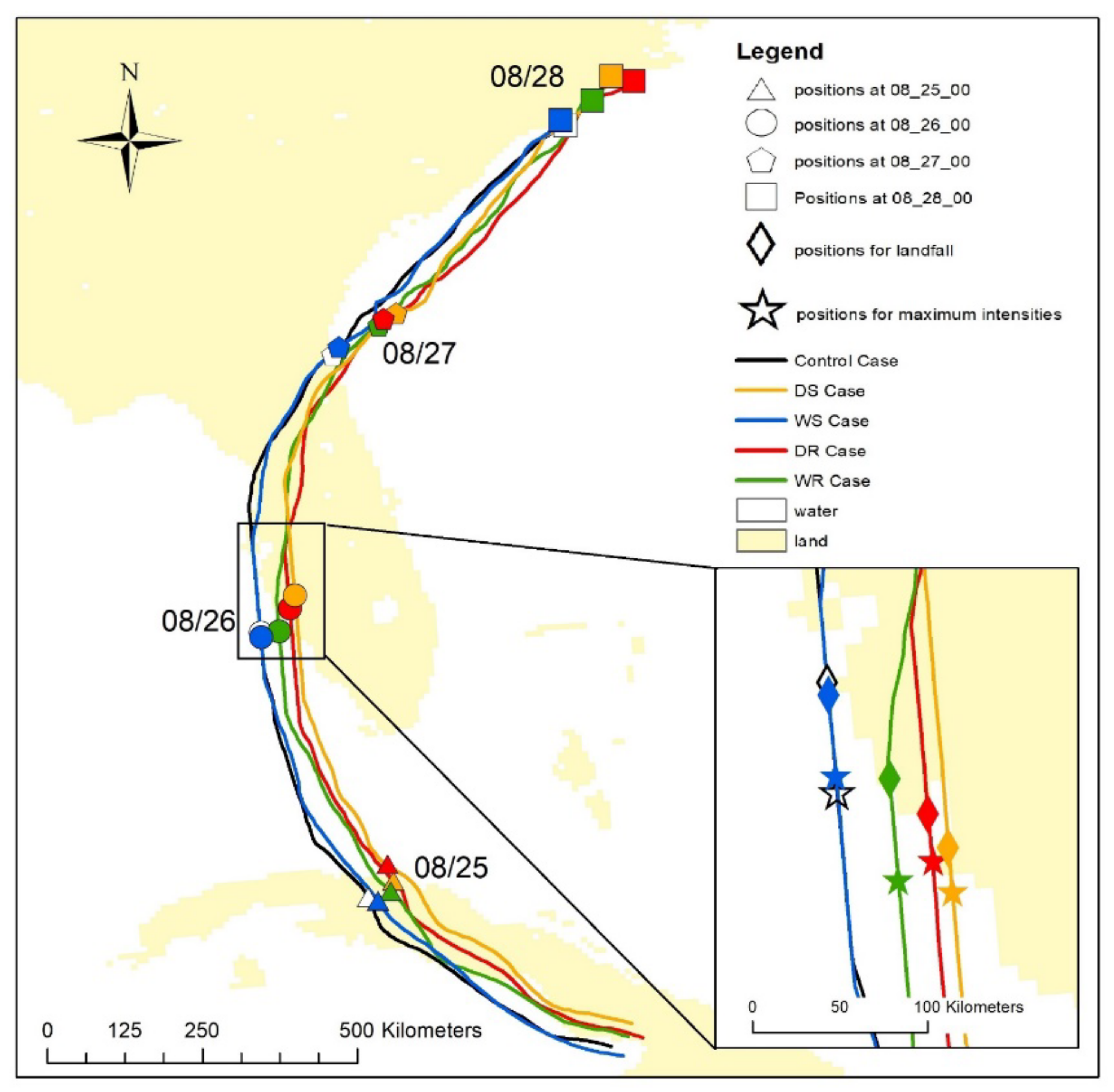
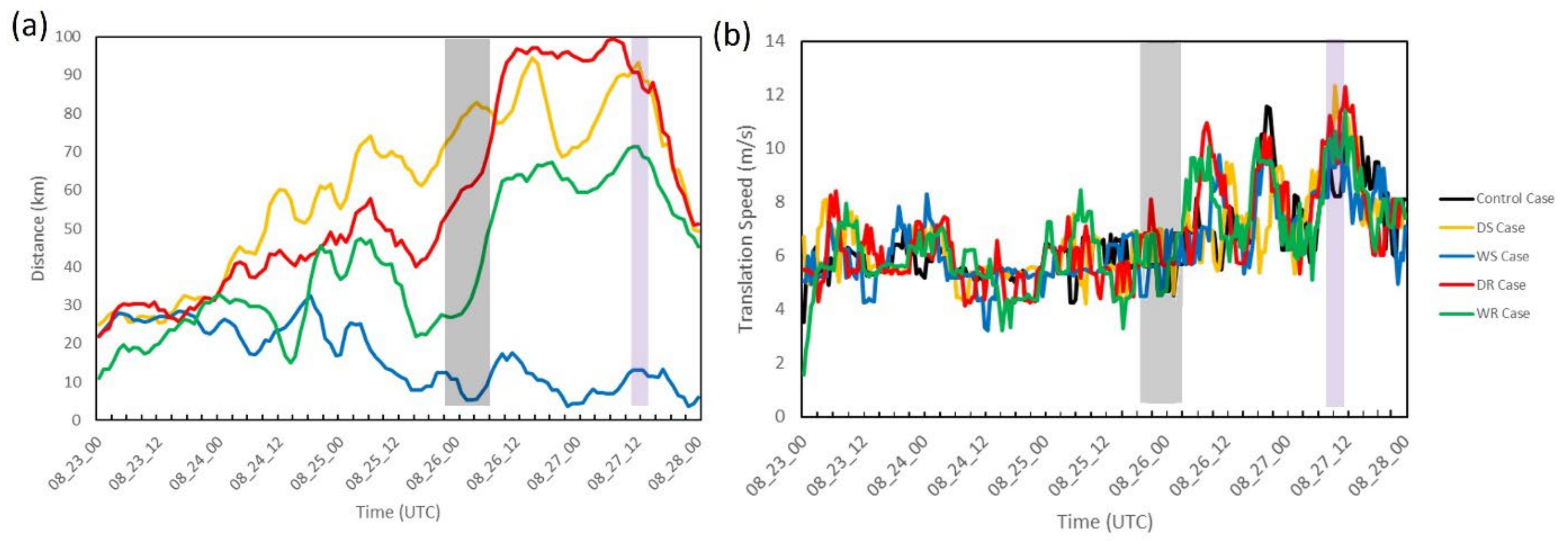
3.1.1. Storm Tracks

We begin by comparing the positions of the storm circulation centers. Figure 2 shows the similarity in the tracks of all five simulations after the storms’ centers move offshore of Cuba. It also depicts the storm locations at the time when each case reaches its maximum intensity. Out of all simulations, Control and WS cases have the most similar tracks (Figure 3a) with the smallest RMSE of 18.52 km. The two dry cases are the most dissimilar to the Control run, with RMSE values approximating 63 km each. In between the dry and WS cases, the WR case has a RMSE of 44.51 km and its path is more similar to those of the dry cases beginning 1800 UTC 24 August (Figure 2). These differences are all relatively small when compared with values ranging from 50 km to 150 km in other studies, e.g., [70,71].
When comparing the locations of Florida landfalls, the Control and WS simulations made landfall approximately 65 to 125 km north of the other three cases. These values are larger than the distance comparisons made at the same time-steps (Figure 3a), because landfalls occur at slightly different times among the cases. The DS case crosses Florida at the southernmost location. All simulations make landfalls within a nine-hour window from 2100 UTC 25 August (DR case) to 0600 UTC 26 August (Control/WS case). After crossing the peninsula, the five simulations leave Florida and move over the North Atlantic Ocean around 0000 UTC 27 August. Next, all simulations make another landfall over South Carolina. For this event, the Control and WS cases make landfalls around Georgetown, where the other three cases make landfall near Myrtle Beach, approximately 100 km northeast of Georgetown. Even though the five simulations do not make landfall at the same locations, the three-hour time range of these landfalls from 1000 UTC (WS Case) to 1300 UTC (DR Case) 27 August is less than for the Florida landfalls.
Figure 3b shows the translation speed among the five simulations. A set of t-tests (results not shown) did not find large differences between cases in translation speed, similar to previous modeling studies of landfalling hurricanes [7,8,15,72]. The translation speed of these storms ranges 5 to 10 m s−1. According to [73], the average speed for their observed Atlantic Basin TCs near landfall is 5.2 m s−1, and our results are also on par with [74], who found a mean motion of 6 m s−1, and a range of 2 to 14 m s−1, in their study of 10 hurricanes from 1982 to 1992.

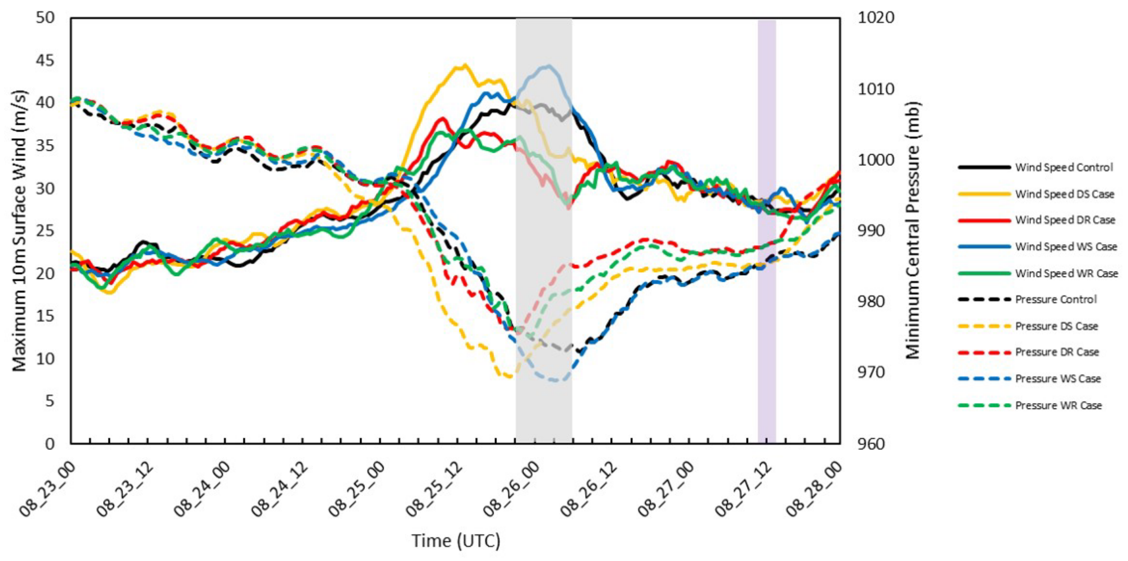
3.1.2. Storm Intensity
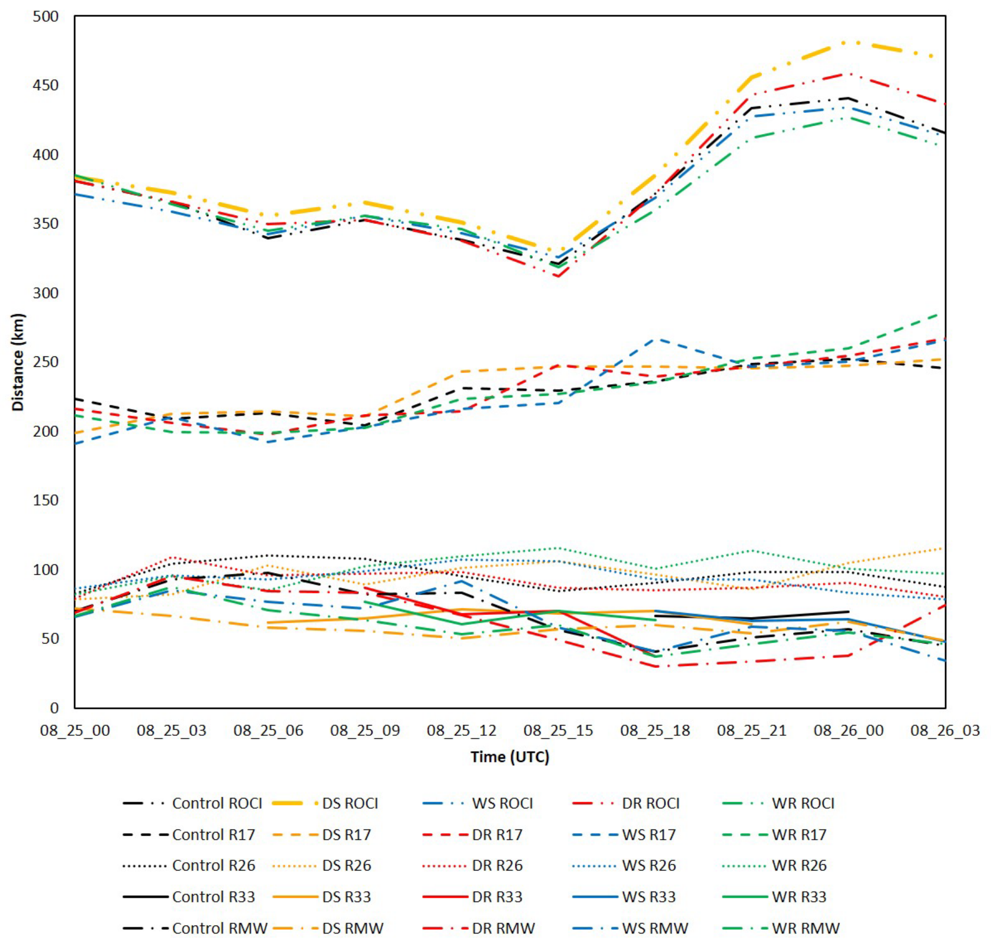
The minimum central pressure at the surface and maximum one-minute sustained wind speed at 10 m (Figure 4) are utilized to compare storm intensity for the period 0000 UTC 23 August, the approximate time the storm reached TS intensity, to 0000 UTC 28 August. We stop at 0000 UTC 28 August because during the last 12 h of the simulation, domain 2 touches the northern boundary of domain 1. All five simulations start as a disturbance around 1200 UTC 20 August. After the land interaction with Cuba, all simulations experience a period of intensification before the third landfall, which is over Florida. Storms have very similar intensity until 0600 UTC 25 August, when the edges of three storms start to have land interaction. After that point, we see differences in rate of intensification and timing of peak intensities. Both smooth cases achieve lower minimum central pressures of 968 mb compared to the Control run (972 mb), while the two rough cases remain approximately 5 mb higher than the Control case. All cases decay while moving across Florida and all centers move back over water by 0000 UTC 27 August.
The majority of the differences in intensity happened from 25 to 27 August (Figure 4), which is also the period in which the storms most interact with the modified land surface. Among the four experiments, WS case has the lowest RMSE from the Control case in both minimum central pressure (1.6 mb) and maximum sustained wind speed (2.2 m s−1). For the other cases, DS case has a slightly larger RMSE than WS with the values of 3.5 mb and 3.0 m s−1. The two rough cases have similar RMSEs that were the highest values of 4.5 mb and 3.2 m s−1. This is consistent with the results of [15], who found that cases with a higher roughness length reduce the surface wind speed more than in lower roughness length cases. Kimball [15] concluded that compared with roughness length, moisture availability does not play as strong of a role in the decay process. Our results are similar in that with identical roughness length, higher moisture availability cases did not show a large difference in either minimum central pressure or maximum one-minute sustained wind speed compared to the less moist cases.
The five simulations attain their highest wind speed from 1200 UTC 25 August to 0300 UTC 26 August. Both smooth cases maintain Category 2 status with maximum sustained wind speed of 45 m s−1 for four hours longer than the Control run, and the two rough cases only reach Category 1 intensity as their highest sustained wind speed is 38 m s−1. DS case reaches maximum intensity first while the Control and WS cases reach maximum intensity last. Even though the five runs reach maximum intensities at slightly different times, they reach maximum intensity at a similar latitude no farther than 75 km from land (Figure 2). Moreover, all of the cases reached maximum intensity within 6 h of their landfall.

3.1.3. Storm Size

It is important to verify that the sizes of the simulated hurricanes are comparable to real TCs in the Atlantic basin to validate the general structure of these simulations. We examine the radius of gale-force winds (R17), damaging force winds (R26), hurricane-force winds (R33), maximum winds (RMW), and outer closed isobar (ROCI) among the five simulations every 3 h during the 30-h period after leaving Cuba, but before the Florida landfall (Figure 5). We limit analysis to this period as after this time, a large part of the storm moves over land, causing an abrupt decrease in wind speed. There is little difference in mean values among all five simulations according to a series of t-tests (results not shown here) for the size metrics. The statistical distribution of all five radii were compared with those reported by [52], which explored statistical properties of size parameters using a dataset spanning 1988–2002 for North Atlantic TCs. Results from the set of t-tests (Table 2) show that, other than R26, the other radii are similar to those in the observational study.

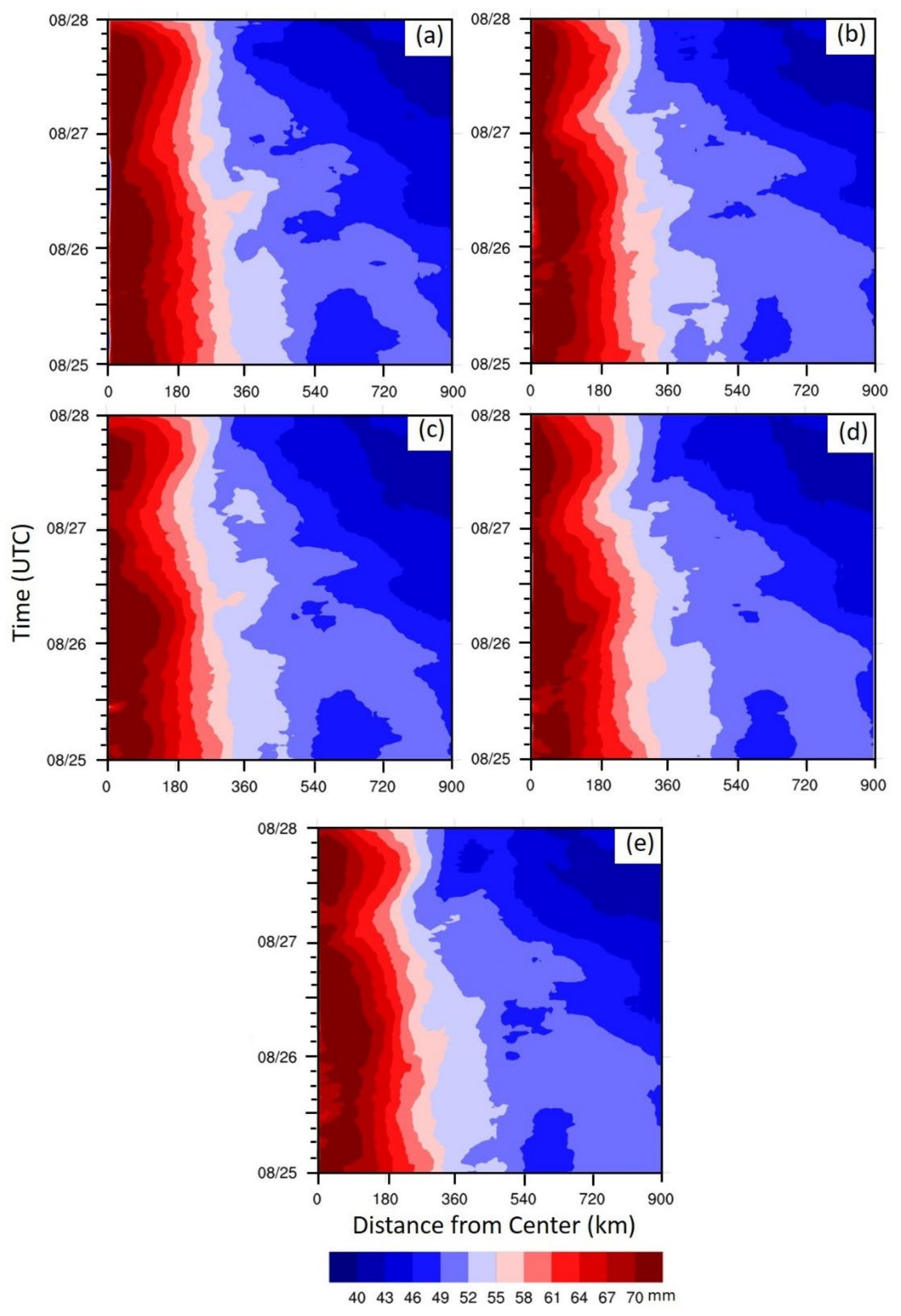
3.1.4. Environmental Moisture
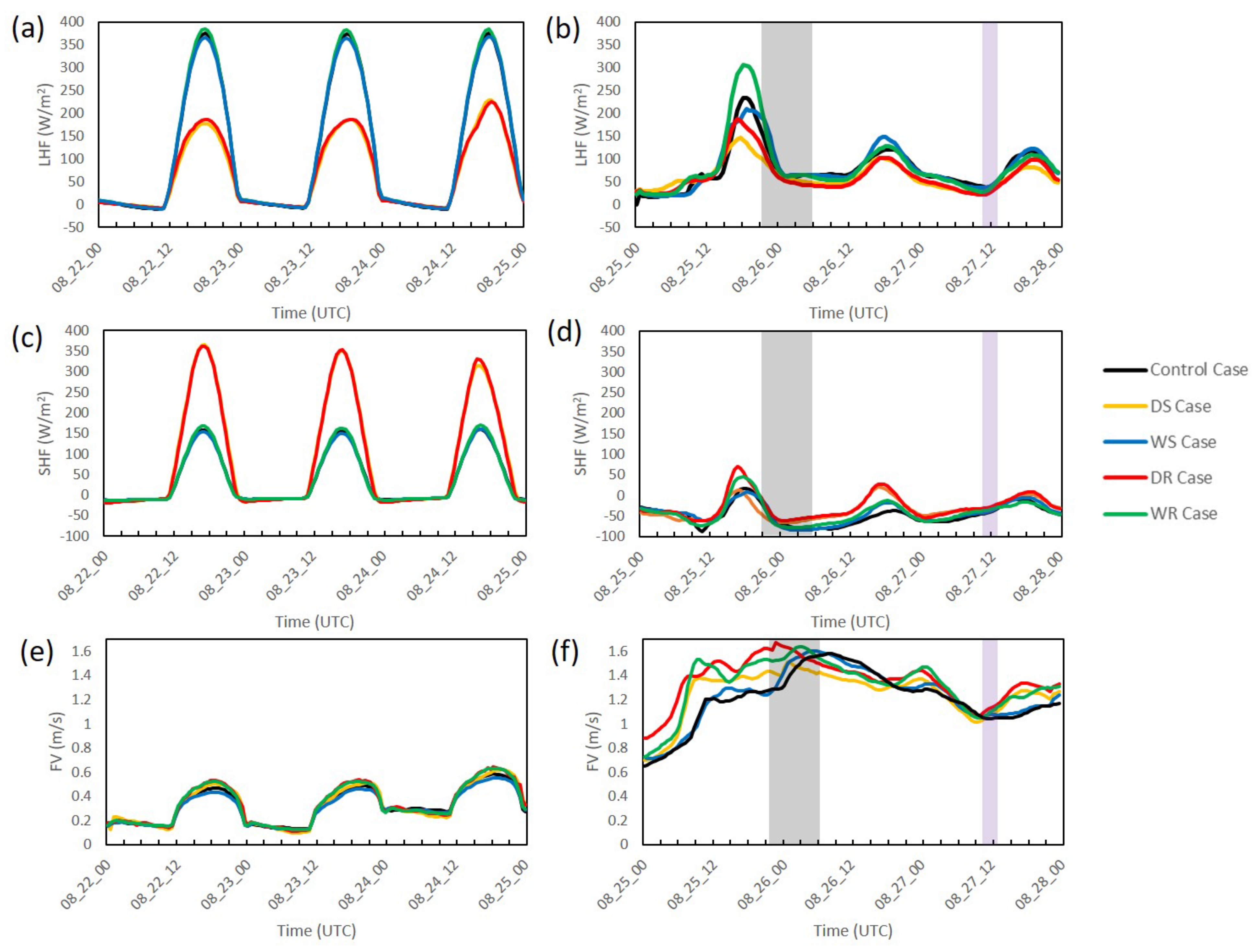
It is also important to verify that all simulations moved through environments with similar distributions of moisture above the boundary layer, so that any differences we detect in the near-land atmosphere among cases are induced by the changes of land surface characteristics instead of synoptic-scale environmental moisture differences. To achieve this goal, we examine the TPW, which has been employed to characterize the environment surrounding TCs in several previous studies [75,76,77]. On average, Atlantic basin TCs encounter TPW ranging from 40 mm to 70 mm [75]. Kim et al. [76] found that TCs approaching Florida’s Gulf coastline tend to encounter TPW values of 50 mm on their right sides, but values could be as low as 35 mm on the left side if a frontal system was interacting with the storm. Figure 6 depicts the spatiotemporal patterns of the five simulations using a Hovmöller diagram, which shows the azimuthal averaged TPW extent out to 900 km from the storm center from 0000 UTC of 25 August to 0000 UTC to 28 August. The highest moisture (over 70 mm) covers the region 0–120 km from the center for all cases. Moreover, TPW outside 360 km decreases from 50 mm to 40 mm over time, which agrees with the fact that the storm is moving northward into the mid-latitudes where drier environments (40–45 mm) normally exist [78]. Overall, the TPW plots reveal reasonable spatial patterns for all cases, and that the synoptic scale environmental moisture content is similar for all cases.

3.2. PBL Variables

3.2.1. PBL Properties before Interaction with the Storm

According to previous studies e.g., [20,23,25,26], in the absence of synoptic-scale forcing (vertical wind speed at 500 mb less than 5 ms−1), land surface evapotranspiration rates are a predominant factor in variations in the near-land atmosphere. Figure 7a,c,e illustrates the trends for LHF, SHF, and FV over land within 150 km from the eventual storm track during the time before the storm (TBS). There is a cycle of increasing values through late morning and decreasing values through early evening, mirroring the diurnal cycle in incoming solar radiation. On 25 August, sunrise occurs at 1105 UTC for Tampa, Florida and sunset occurs at 2358 UTC. Values are much lower and little variability exists among the cases when solar radiation is absent. In addition to performing a Kruskal–Wallis test on values for all times, we also test times 1100—0000 UTC that encompass daylight hours.
Due to the similarity of values during the night, minimal differences exist among TBS values when all times are considered (Table 3). However, values during the day yield larger differences and thus paired tests are conducted (Table 4). As expected, the Control and Wet cases yield higher latent heat flux values, while the dry cases yield higher sensible heat values. Peak values of LHF for wet and the Control cases are >140 W m−2 than those for dry cases. On the other hand, the SHF values for dry cases nearly double those for the Control and wet cases when all cases peak at 1700 UTC (1:00 pm LST). In terms of FV, the rough cases have the highest values, while WS and Control produce the lowest values. The DS values are closer to the rough cases than WS or Control.

3.2.2. PBL Properties during Interaction with the Storm

The previous section confirmed that in the absence of synoptic-scale forcing, the near-surface atmospheric variables had values that differed according to the modified land surface characteristics. Next, we examine conditions over land areas within 150 km of the storm track while winds are at least gale-force (TDS). Overall, we can still identify differences between the cases, but the magnitudes are smaller compared with TBS as expected for LHF and SHF (Figure 7b,d) and larger for FV (Figure 7f). Among the three days, 25 August contains the highest values in both variables. This result can be explained by the fact that the storms are reaching their maximum intensity, so there are increases in the wind speed which have a positive influence on these variables. Moreover, the land is located on the right side of the storm during 25 August whereas for the next two days, the land is mainly located on the left side of the storm (Figure 2), especially after 1200 UTC 26 August. As TCs in the northern hemisphere have stronger wind on the right side of the storm, the wind speed should be even lower over land 26 and 27 August, compared with 25 August. Although less pronounced, the diurnal cycle is still visible for LHF and SHF. The maximum value of LHF is 385 W m−2 for TBS compared with 307 W m−2 for TDS and maximum value for SHF is 365 W m−2 for TBS and only 70 W m−2 for TDS. The change in the magnitude of these heat fluxes can be accounted for by two primary processes. First, the cloud cover of the TC reduces the incoming solar radiation, which reduces the overall incoming heat energy. Second, strong winds associated with the TC throughout the PBL promote mixing so that conditions at surface are different than in a more quiescent environment. The higher wind speeds lead to higher values of FV [79] and as the TC center approaches land in the simulations, this leads to an increase in for FV in all cases.
Though the magnitudes of the heat fluxes are reduced, differences still exist between cases regardless of whether all times or daylight times are examined (Table 3). As the pairwise comparisons produce similar results when all or just daylight times are compared, we present results for the daylight tests in Table 5 to be directly comparable with Table 4 for TBS. Although the Control and two wet cases are very similar, both SHF and LHF show differences between wet cases and dry cases that are significant at the 95% confidence level, echoing the findings for TBS. The one difference for TDS compared to TBS is that the p-values are larger in tests for which the null hypothesis cannot be rejected. Thus, we assert that our modification of the land surface affects heat fluxes in the PBL despite the stronger synoptic-scale flow and mixing that occur during a TC. However, there is little difference between smooth and rough cases with same moisture level. This can be caused by the mixed influence of increased roughness length, which can increase the surface exchange coefficient that positively influences the heat fluxes terms. In the meantime, the increased friction may greatly reduce the surface wind speed, which can reduce the heat fluxes.
Friction velocity is another fundamental parameter in several processes of the PBL, especially those linked to the vertical transport of momentum, or turbulence generation, which helps lift extra LHF and SHF into the storm from the land. Values of FV increase for TDS as compared to TBS, and the increased mixing can help explain why the diurnal cycle is less pronounced for LHF and SHF during the TC’s passage. Increased FV values occur at night as well as in the day during storm passage, while a more pronounced diurnal variation occurs TBS. The higher FV values for TDS also allow more variation to occur among the cases, and we find that the null hypothesis can be rejected with 95% confidence in eight comparisons as opposed to four in the TBS. The rough cases still have the highest median values for FV (1.39 m s−1 for DR and 1.36 m s−1 for WR), but they are more distant from the values in Control (1.25 m s−1) and WS (1.27 m s−1) cases than TBS, and the DS case which has the third highest median (1.33 m s−1) and is dissimilar to all other cases. The one test whose results change when all hours are considered for TDS is the comparison for WS and DS cases; there, the null hypothesis cannot be rejected based on a p-value of 0.29. This implies that WS and DS are more similar in the absence of solar radiation.
A consistent result across all times and both periods is that WS and Control cases have similar values for LHF, SHF, and FV. This result supports our hypothesis that WS and Control cases have the most similar results, which we base on comparisons to actual values for different vegetation and soil moisture types. Recall that the average moisture availability for the Control case is 42%, and roughness length is 30.2 cm. Given that their tracks are also the most similar, we hypothesize that the precipitation patterns for WS and Control will also be similar. As for the WR case, it does not show consistently higher values in LHF than the other two wet cases. This can be due to the mixed effects of increased upward momentum and decreased surface wind speed caused by increased roughness length. DS and DR cases are similar in SHF and LHF, while DR is more similar to WR in FV.

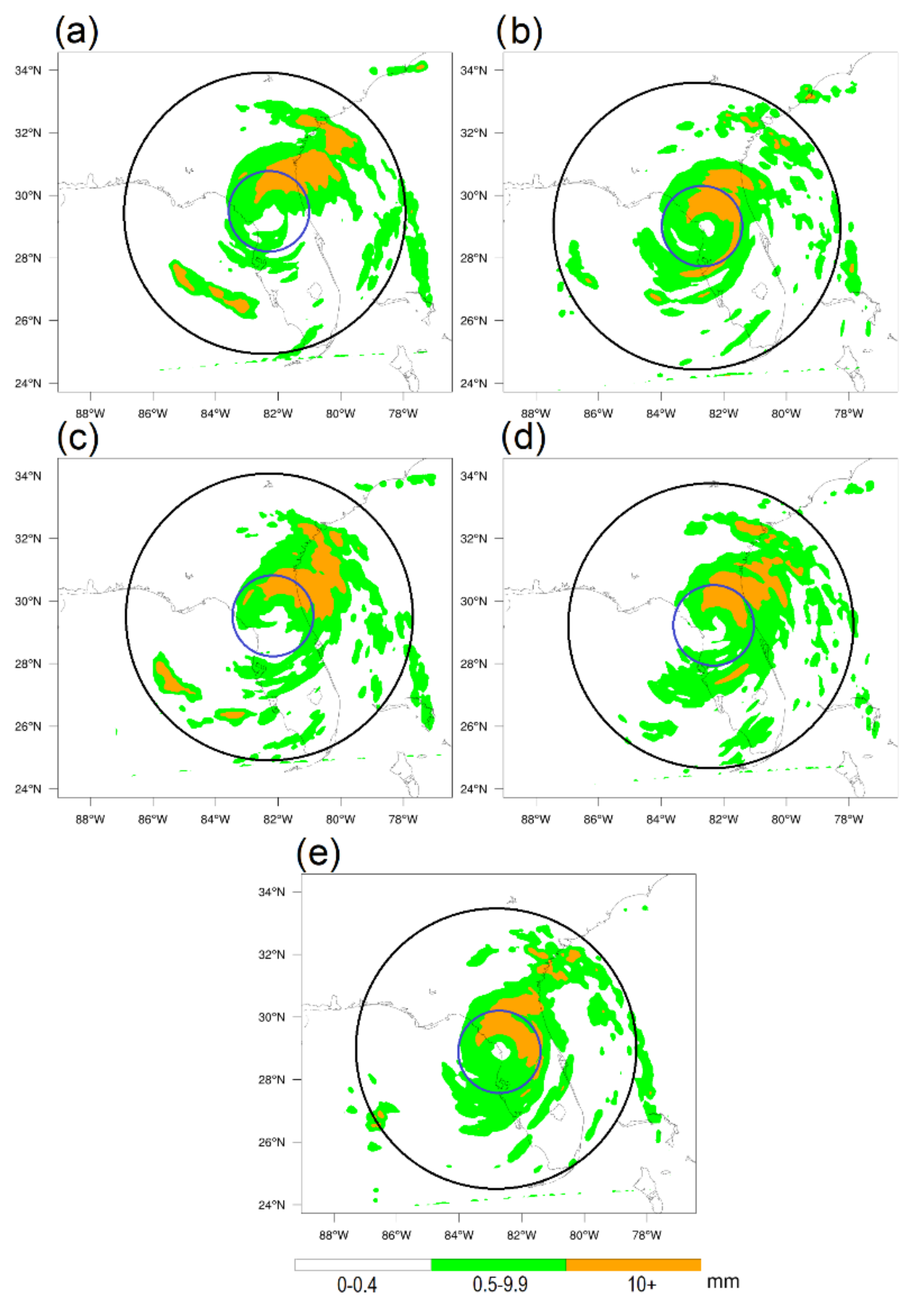
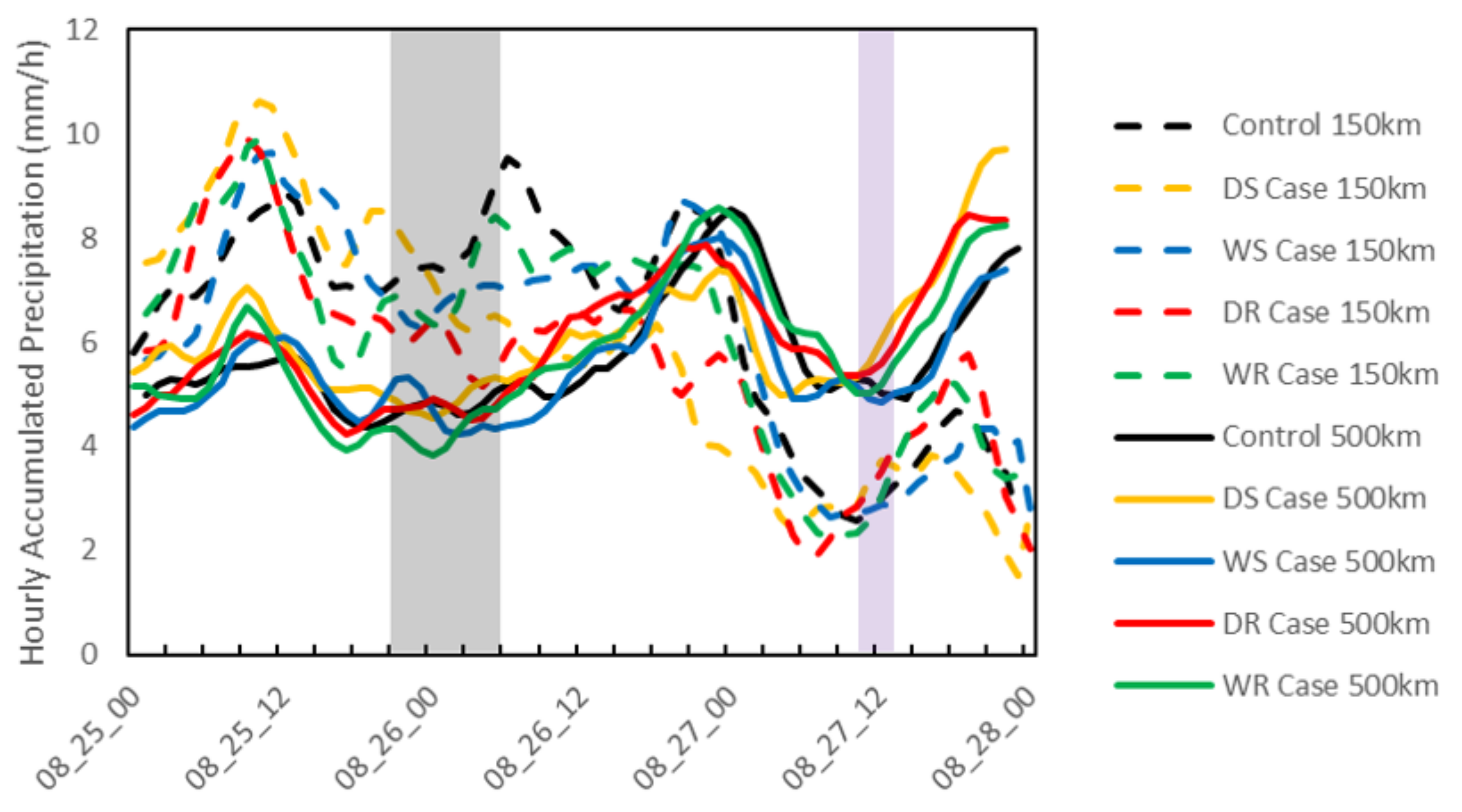
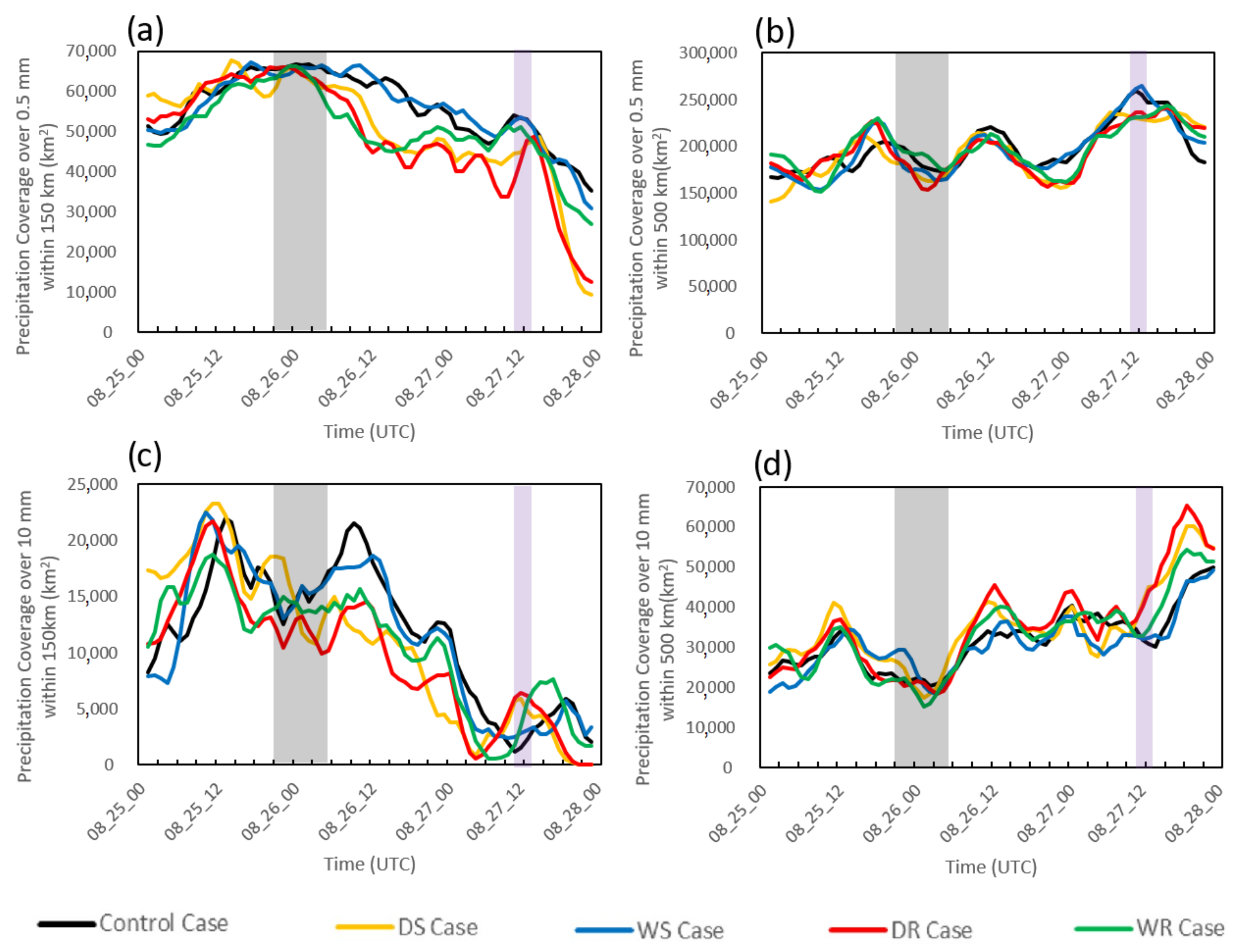
3.3. Precipitation Accumulation and Area

To place the precipitation analysis into spatial context, it should be noted that the Florida peninsula is < 250 km wide (Figure 1), meaning that most of the outer region is over water at the time of landfall. Much of the rear of the storm is over the Gulf of Mexico, while the front of the storm is over the Atlantic Ocean. Much of the left front quadrant remains over land, however, and precipitation likely develops in the outer region due to convergence of moist air sourced from over the Atlantic Ocean along the coastlines of Georgia and South Carolina (Figure 8).
We begin by examining areal-averaged precipitation accumulation values. Figure 9 shows the hourly precipitation accumulation for non-zero grid cells averaged over the area within 150 and 500 km from the storm center through our three-day window of interaction with the modified land surface. Hourly totals within both distances reach a relative peak between 0900 UTC to 1200 UTC 25 August near the times of TC maximum intensity prior to landfall, and accumulations decrease from that point until landfall. Precipitation in the larger radius is 2–4 mm h−1 lower than that in the core. After Florida landfall, overall trends in the inner core and outer region oppose one another over the next 24 h. The precipitation amount in the inner core decreases, particularly for the dry cases, while all cases exhibit a steady increase when the outer region is included. The slowing of winds (Figure 3) leading to less convergence could explain the decrease in the core, along with the fact that rainfall tends to spread outwards from the circulation center as a TC tracks inland [15]. This spreading would help increase precipitation in the outer region. Additionally, increased convergence occurs due to friction along the Georgia and South Carolina coasts, helping to increase precipitation in this area.
Moving forward, the accumulations in the outer region peak around 0000 UTC 27 August, and values are similar for the outer region in all cases as well as for the Control and wet cases of the inner core. Values decrease in both regions over the next 6–9 h, although values are now higher for the whole region than the inner core area and remain so for the rest of the day. The increasing trend for both distances from 0300—1800 UTC 27 August coincides with the landfall over South Carolina. Here, the increased friction on the left side of the storm and the ample moisture advecting into the right side of the storm from over the Atlantic Ocean likely combine to enhance precipitation.
Statistical tests show that mean accumulations differ when the inner core is considered, but are much more similar when the entire 500-km region is examined (Table 6). Thus, a set of paired tests compare values between cases for the 150 km region only (Table 7). The Control and two wet cases have similar accumulations, and accumulations are higher than those for the dry cases. The dry cases also have accumulations that are similar with each other. The higher values occur in the day after landfall (Figure 9) when the inner core has the most interaction with the modified land surface, suggesting that the modified land surface contributed to this peak, while values become more similar once the TC’s core moves over the Atlantic Ocean. Further evidence that our modified land surface could be influencing precipitation can be found when comparing these results to those for LHF during the storm’s passage. Nine out of ten tests produce similar results when comparing LHF (Table 5) and accumulations within the 150 km radius (Table 7). The one different result is that while the Control and WR cases have similar values for LHF, Control has higher precipitation accumulations than WR case, especially in the hours right after landfall. This can be explained by the fact that the Control case spends more time over water before landfall and thus reached a higher intensity, allowing it to evaporate more moisture to then be condensed into precipitation in the hours immediately following landfall.
We now examine the time series of precipitation coverage for 0.5 mm h−1 and 10 mm h−1 thresholds for the 150 km and 500 km regions (Figure 10). For reference, 100% coverage for the 150 (500) km region equates to 70,650 (785,000) sq. km. We begin with the 0.5 mm h−1 threshold where precipitation coverage seems to equate more with storm intensity for the inner region, while the diurnal cycle is more apparent in the outer region. An increasing trend occurs from 0000 UTC 25 August until landfall time in all cases within 150 km radius (Figure 10a), which coincides with storm intensification. After landfall, the areal coverages of all cases generally decreases until 28 August, which is also when the storm loses strength. These results support the observational study of [80] who found rainfall strength to be strongly related to TC intensity. For the 500 km radius (Figure 10b), there is a noticeable diurnal cycle, where growth starts around 0000 UTC and peaks around 1200 UTC. This can be explained by the fact that there is a lag between rain-field growth and increasing moisture from the surface during the previous 12 h [36]. It is around 1200 UTC when the LHF starts to increase due to increasing incoming solar radiation. As most of the 500 km region does not contain precipitation, the lack of cloud cover allows insolation to reach the land surface. On the other hand, most of the inner core is covered by precipitation, and therefore clouds reflect a significant portion of insolation, save for in the TC’s eye (Figure 8e). This is particularly true for the WS and Control cases with their corresponding higher coverage (Figure 10a) from landfall until the end of the study period. The high amount of cloud cover likely explains the lack of a pronounced diurnal cycle in the 150 km region.
From the 0.5 mm h−1 threshold, more differences in areal coverage exist among the simulations within the 150 km than the 500 km radius, as shown in the Kruskal–Wallis tests (Table 6). Control and WS cases are similar (Table 7) and have higher median values when compared to the other three cases. These higher values occur during the 36 h after the Florida landfall (Figure 10a). The other three cases are similar to each other. Again, the fact that the largest differences occur after landfall when the core interacts with land provides support to the hypothesis that the modified land surface helped to produce differences in precipitation rather than the differences being due to random chance. It should be noted that the WR case is more different from the Control case in the current test than it was in the earlier test for rain accumulation (Table 6). The track of WR is closer to the two dry cases (RMSE values < 25 km) than Control and WS cases (RMSE values > 33 km) (Figure 2). The two dry and WR cases achieved maximum intensity and made landfall at similar times and locations as well. It is right after landfall that the WR case exhibits similar trends with the DR and DS cases (Figure 10a).
For the 10 mm h−1 threshold, Control and wet cases again have higher values than the dry cases for the 150 km radius (Table 7). The largest differences compared to the other cases occur during 26 August (Figure 10c). All cases have their lowest values on 27 August when high rain rates move outwards. Interestingly, test results for 500 km radius show that dry and rough cases have higher medians than the Control and WS cases; this happens on 26–28 August (Figure 10d). These higher coverages occur due the increased roughness length, and therefore friction velocity for rough cases and the increased moisture gradient for the dry cases in the outer rainbands and along the coastline are seen in Figure 8.

4. Discussion and Conclusions

This paper illustrated the linkages among land surface conditions, PBL variables, and precipitation production in simulated landfalling hurricanes. The WRF model was run with data from the Hurricane Nature Run 2, which featured landfalls over Florida and South Carolina. Following the Control run that incorporated the actual heterogeneous land surface, four additional simulations were performed after altering the moisture availability and roughness length of the land surface. These simulations featured homogeneous surfaces that were wet/rough, wet/smooth, dry/rough, and dry/smooth. We first compared our modeled storms to each other and other Atlantic Basin TCs to confirm that our TCs were realistic in track, intensity, and size. We then analyzed three PBL variables before and during the storm’s passage: latent heat flux, sensible heat flux, and friction velocity. At last, we examined hourly precipitation accumulations and the area of 0.5 mm hr−1 and 10 mm hr−1 accumulations within the storm’s core and over its entire circulation to determine how coverages of low and high rain rates evolved among the simulations as the TCs moved over land.
Before the storm interacted with modified land surface, wet (dry) cases had higher values for latent (sensible) heat fluxes (p > 0.05) in the daytime, while rough cases had higher values in FV than smooth cases as expected. While the storm moved over the modified land surface, statistically significant differences still existed in the medians of all of the three PBL variables, though the values of LHF and SHF were lower compared with before storm interaction, while FV had more variation due to the increased surface wind speed. These results agree well with previous studies [20,24] and suggest that the land surface condition was the dominant factor influencing the near surface atmosphere when surface winds were weak. In building on the work of [17], our results showed that during stronger synoptic-scale events, such as the passage of a TC, atmospheric response in heat fluxes was smaller, yet still detectable. Thus, it is also important to take land surface characteristics into consideration when forecasting precipitation under stronger synoptic forcing, as the land surface may still influence the PBL.
In terms of rainfall, differences were maximized among the simulations when activity within 150 km of the storm center was considered. When analyzing rainfall accumulation and area covered by lower and higher rain rates in this region, Control and WS simulations exhibited similarly high values, while values were lower for the dry cases. This approximates the results from the analysis of latent heat flux. The timing of the highest values as the storm cores moved over Florida suggests that the higher moisture availability in the control and wet simulations could have enhanced rainfall production. When examining areas receiving higher rain rates within 500 km of the storm center, a different result occurs, as the rough and dry cases exhibit the largest values. The higher values occurred when the TC outer rainbands interacted with the coastline. Near this boundary, the dry cases would have a greater moisture gradient than the moist cases, and friction velocity was higher for the rough cases than for the dry cases. Both situations could have enhanced rain rates and support the hypothesis that modifying the moisture availability and surface roughness can affect precipitation production in a landfalling TC.
There are two main limitations to this analysis. First, even though our study identified differences in the precipitation patterns of a landfalling TC in a realistic atmospheric setting, we modified land surface into an unrealistic homogenous surface. Thus, our results provide limited implications for strategies in managing land cover and land use to reduce extreme precipitation during TC passage. Thus, future research should examine more heterogeneous land surfaces. Second, HNR2 only passed over a 250 km-wide section of Florida and then moved along the coastline of Georgia and South Carolina, thus it remained near the oceanic source of latent heat. As a result, modifications to moisture availability by this land surface sensitivity analysis may not have played as important a role in changing the overall amount of the precipitation compared to what could have been observed had the storm moved directly inland. Thus, future studies should examine realistic conditions for TCs that move directly inland.
Finally, although comparing the precipitation coverage within the inner core and entire circulation separately provided useful insights of the rainfall distribution compared with the precipitation amount, this method averaged data over a large region which limits the ability to discern fine-scale differences. For example, the largest 10 mm hr−1 threshold rainfall areas are along the Georgia and South Carolina coastline, but the shape of the largest area in the WR case is quite different from the WS case. In future studies, we will measure the spatial properties of the precipitation regions, such as the width of the rainfall swath and the tangential coverage around the storm center, to more accurately compare the simulation outputs.

Author Contributions

Conceptualization, Y.W. and C.J.M.; methodology, Y.W. and C.J.M.; validation, Y.W.; formal analysis, Y.W.; data curation, Y.W.; writing—original draft preparation, Y.W.; writing—review and editing, C.J.M.; visualization, Y.W.; supervision, C.J.M.; project administration, C.J.M.; funding acquisition, C.J.M. All authors have read and agreed to the published version of the manuscript.

Funding

This research was funded by The National Science Foundation, grant number BCS-1053864. High-performance computing support from Yellowstone (ark:/85065/d7wd3xhc) was provided by NCAR’s Computational and Information Systems Laboratory, sponsored by the National Science Foundation.

Institutional Review Board Statement

Not applicable.

Informed Consent Statement

Not applicable.

Data Availability Statement

Sample output data from the simulations have been deposited to the University of Florida Institutional Repository. https://original-ufdc.uflib.ufl.edu/l/IR00011701/00001" https://original-ufdc.uflib.ufl.edu/l/IR00011701/00001, accessed on 11 January 2022.

Acknowledgments

David Nolan provided the data and source code to perform the Control simulation. Michael Bell, Jingyin Tang, and Stephanie Zick provided feedback about the experimental design.

Conflicts of Interest

The authors declare no conflict of interest. The funders had no role in the design of the study; in the collection, analyses, or interpretation of data; in the writing of the manuscript, or in the decision to publish the results.

References

  1. Malkus, J.S.; Rhiel, H. On the dynamics and energy transformations in steady-state hurricanes. Tellus 1960, 12, 1–20. [Google Scholar] [CrossRef] [Green Version]
  2. Gamache, J.F.; Houze, R.A.; Marks, F.D. Dual-aircraft investigation of the inner-core of Hurricane Norbert.3. Water-budget. J. Atmos. Sci. 1993, 50, 3221–3243. [Google Scholar] [CrossRef] [Green Version]
  3. Trenberth, K.E.; Davis, C.A.; Fasullo, J. Water and energy budgets of hurricanes: Case studies of Ivan and Katrina. J. Geophys. Res. Atmos. 2007, 112, 11. [Google Scholar] [CrossRef]
  4. Andersen, T.K.; Radcliffe, D.E.; Shepherd, J.M. Quantifying surface energy fluxes in the vicinity of inland-tracking tropical cyclones. J. Appl. Meteorol. Climatol. 2013, 52, 2797–2808. [Google Scholar] [CrossRef]
  5. Shepherd, J.; Thomas, A.; Santanello, J.; Lawston-Parker, P.; Basara, J. Evidence of warm core structure maintenance over land: A case study analysis of cyclone Kelvin. Environ. Res. Commun. 2021, 3, 045004. [Google Scholar] [CrossRef]
  6. Arndt, D.S.; Basara, J.B.; McPherson, R.A.; Illston, B.G.; McManus, G.D.; Demko, D.B. Observations of the overland reintensification of Tropical Storm Erin (2007). Bull. Amer. Meteor. Soc. 2009, 90, 1079–1093. [Google Scholar] [CrossRef]
  7. Tuleya, R.E. Tropical storm development and decay: Sensitivity to surface boundary-conditions. Mon. Weather Rev. 1994, 122, 291–304. [Google Scholar] [CrossRef] [Green Version]
  8. Tuleya, R.E.; Bender, M.A.; Kurihara, Y. A simulation study of the landfall of tropical cyclones using a movable nested-mesh model. Mon. Weather Rev. 1984, 112, 124–136. [Google Scholar] [CrossRef] [Green Version]
  9. Tuleya, R.E.; Kurihara, Y. A numerical simulation of the landfall of tropical cyclones. J. Atmos. Sci. 1978, 35, 242–257. [Google Scholar]
  10. Andersen, T.K.; Shepherd, J.M. A spatio-temporal analysis of tropical cyclone maintenance or intensification inland. Int. J. Climatol. 2013, 10, 1002–1013. [Google Scholar] [CrossRef]
  11. Emanuel, K.; Callaghan, J.; Otto, P. A hypothesis for the redevelopment of warm-core cyclones over Northern Australia. Mon. Weather Rev. 2008, 136, 3863–3872. [Google Scholar] [CrossRef]
  12. Evans, C.; Schumacher, R.S.; Galarneau, T.J. Sensitivity in the overland reintensification of Tropical Cyclone Erin (2007) to near-surface soil moisture characteristics. Mon. Weather Rev. 2011, 139, 3848–3870. [Google Scholar] [CrossRef] [Green Version]
  13. Nair, U.S.; Rappin, E.; Foshee, E.; Smith, W.; Pielke, R.A.; Mahmood, R.; Case, J.L.; Blankenship, C.B.; Shepherd, M.; Santanello, J.A.; et al. Influence of land cover and soil moisture based brown ocean effect on an extreme rainfall event from a Louisiana Gulf Coast tropical system. Sci. Rep. 2019, 9, 17136. [Google Scholar] [CrossRef]
  14. Shen, W.X.; Ginis, I.; Tuleya, R.E. A numerical investigation of land surface water on landfalling hurricanes. J. Atmos. Sci. 2002, 59, 789–802. [Google Scholar] [CrossRef] [Green Version]
  15. Kimball, S.K. Structure and evolution of rainfall in numerically simulated landfalling hurricanes. Mon. Weather Rev. 2008, 136, 3822–3847. [Google Scholar] [CrossRef]
  16. Pielke, R. Comparison of 3 dimensional versus 2 dimensional numerical predictions of sea breezes over South Florida. Bull. Amer. Meteorol. Soc. 1973, 54, 752. [Google Scholar]
  17. Quintanar, A.I.; Mahmood, R.; Suarez, A.; Leeper, R. Atmospheric sensitivity to roughness length in a regional atmospheric model over the Ohio-Tennessee River Valley. Meteorol Atmos Phys 2016, 128, 315–330. [Google Scholar] [CrossRef]
  18. Avissar, R.; Pielke, R.A. A parameterization of heterogeneous land surfaces for atmospheric numerical-models and its impact on regional meteorology. Mon. Weather Rev. 1989, 117, 2113–2136. [Google Scholar] [CrossRef] [Green Version]
  19. Eltahir, E.A.B.; Pal, J.S. Relationship between surface conditions and subsequent rainfall in convective storms. J. Geophys. Res.-Atmos. 1996, 101, 26237–26245. [Google Scholar] [CrossRef]
  20. Pielke, R.A. Influence of the spatial distribution of vegetation and soils on the prediction of cumulus convective rainfall. Rev. Geophys. 2001, 39, 151–177. [Google Scholar] [CrossRef]
  21. Brunsell, N.A. Characterization of land-surface precipitation feedback regimes with remote sensing. Remote Sens. Environ. 2006, 100, 200–211. [Google Scholar] [CrossRef]
  22. Matsui, T.; Lakshmi, V.; Small, E.E. The effects of satellite-derived vegetation cover variability on simulated land-atmosphere interactions in the NAMS. J. Clim. 2005, 18, 21–40. [Google Scholar] [CrossRef]
  23. De Ridder, K. The impact of vegetation cover on sahelian drought persistence. Bound. Layer Meteor. 1998, 88, 307–321. [Google Scholar] [CrossRef]
  24. Matyas, C.J.; Carleton, A.M. Surface radar-derived convective rainfall associations with Midwest US land surface conditions in summer seasons 1999 and 2000. Theor. Appl. Climatol. 2010, 99, 315–330. [Google Scholar] [CrossRef]
  25. Trier, S.B.; Davis, C.A. Mesoscale convective vortices observed during BAMEX. Part II: Influences on secondary deep convection. Mon. Weather Rev. 2007, 135, 2051–2075. [Google Scholar] [CrossRef] [Green Version]
  26. Dyer, J.L.; Rigby, J.R. Assessing the sensitivity of lower atmospheric characteristics to agricultural land use classification over the Lower Mississippi River Alluvial Valley. Theor. Appl. Climatol. 2020, 142, 305–320. [Google Scholar] [CrossRef]
  27. Dorman, J.L.; Sellers, P.J. A global climatology of albedo, roughness length and stomatal-resistence for atmospheric general-circulation models as represented by the simple biosphere model (SIB). J. Appl. Meteorol. 1989, 28, 833–855. [Google Scholar] [CrossRef] [Green Version]
  28. Zha, J.L.; Zhao, D.M.; Wu, J.; Zhang, P.W. Numerical simulation of the effects of land use and cover change on the near-surface wind speed over Eastern China. Clim. Dyn. 2019, 53, 1783–1803. [Google Scholar] [CrossRef]
  29. Lyons, T.J.; Smith, R.C.G.; Xinmei, H. The impact of clearing for agriculture on the surface energy budget. Int. J. Climatol. 1996, 16, 551–558. [Google Scholar] [CrossRef] [Green Version]
  30. Segal, M.; Garratt, J.R.; Kallos, G.; Pielke, R.A. The impact of wet soil and canopy temperatures on the daytime boundary-layer growth. J. Atmos. Sci. 1989, 46, 3673–3684. [Google Scholar] [CrossRef]
  31. Chen, F.; Avissar, R. Impact of land-surface moisture variability on local shallow convective cumulus and precipitation in large-scale models. J. Appl. Meteorol. 1994, 33, 1382–1401. [Google Scholar] [CrossRef] [Green Version]
  32. Li, X.; Mitra, C.; Dong, L.; Yang, Q.C. Understanding land use change impacts on microclimate using Weather Research and Forecasting (WRF) model. Phys. Chem. Earth 2018, 103, 115–126. [Google Scholar] [CrossRef]
  33. Yang, L.; Smith, J.A.; Baeck, M.L.; Bou-Zeid, E.; Jessup, S.M.; Tian, F.Q.; Hu, H.P. Impact of urbanization on heavy convective precipitation under strong large-scale forcing: A case study over the Milwaukee-Lake Michigan region. J. Hydrometeorol. 2014, 15, 261–278. [Google Scholar] [CrossRef]
  34. Rogers, R.F.; Davis, R.E. The effect of coastline curvature on the weakening of Atlantic tropical cyclones. Int. J. Climatol. 1993, 13, 287–299. [Google Scholar] [CrossRef]
  35. Konrad, C.E.; Meaux, M.F.; Meaux, D.A. Relationships between tropical cyclone attributes and precipitation totals: Considerations of scale. Int. J. Climatol. 2002, 22, 237–247. [Google Scholar] [CrossRef]
  36. Matyas, C.J. Processes influencing rain-field growth and decay after tropical cyclone landfall in the United States. J. Appl. Meteorol. Climatol. 2013, 52, 1085–1096. [Google Scholar] [CrossRef]
  37. Ding, L.D.; Li, T.; Xiang, B.Q.; Peng, M.L.D. On the westward turning of Hurricane Sandy (2012): Effect of atmospheric intraseasonal oscillations. J. Clim. 2019, 32, 6859–6873. [Google Scholar] [CrossRef]
  38. Evans, J.L.; Allan, R.J. El-Nino Southern Oscillation modification to the structure of the monsoon and tropical cyclone activity in the Australasian region. Int J. Climatol. 1992, 12, 611–623. [Google Scholar] [CrossRef]
  39. Kikuchi, K.; Wang, B. Formation of tropical cyclones in the northern Indian Ocean associated with two types of tropical intraseasonal oscillation modes. J. Meteorol. Soc. Jpn. 2010, 88, 475–496. [Google Scholar] [CrossRef] [Green Version]
  40. Chen, X.Y.; Wu, L.G. Topographic influence on the motion of tropical cyclones landfalling on the coast of China. Weather. Forecast. 2016, 31, 1615–1623. [Google Scholar] [CrossRef]
  41. Bender, M.A.; Ginis, I. Real-case simulations of hurricane-ocean interaction using a high-resolution coupled model: Effects on hurricane intensity. Mon. Weather Rev. 2000, 128, 917–946. [Google Scholar] [CrossRef]
  42. Ma, Z.H.; Fei, J.F.; Huang, X.G.; Cheng, X.P. Modulating effects of mesoscale oceanic eddies on sea surface temperature response to tropical cyclones over the western North Pacific. J. Geophys. Res. Atmos. 2018, 123, 367–379. [Google Scholar] [CrossRef]
  43. Reale, O.; Terry, J.; Masutani, M.; Andersson, E.; Riishojgaard, L.P.; Jusem, J.C. Preliminary evaluation of the European Centre for Medium-Range Weather Forecasts’ (ECMWF) Nature Run over the tropical Atlantic and African monsoon region. Geophys. Res. Lett. 2007, 34. [Google Scholar] [CrossRef] [Green Version]
  44. Andersson, E.; Masutani, M. Collaboration on observing system simulation experiments (Joint OSSE). ECMWF Newsl. 2010, 123, 14–16. [Google Scholar]
  45. Nolan, D.S.; Atlas, R.; Bhatia, K.T.; Bucci, L.R. Development and validation of a hurricane nature run using the joint OSSE nature run and the WRF model. J. Adv. Modeling Earth Syst. 2013, 5, 382–405. [Google Scholar] [CrossRef]
  46. Nolan, D.S.; Mattocks, C.T. Development and evaluation of the second hurricane nature run Using the Joint OSSE Nature Run and the WRF model. In Proceedings of the 31st Conference on Hurricanes and Tropical Meteorology, San Diego, CA, USA, 31 March–4 April 2014. [Google Scholar]
  47. Jiang, H.; Liu, C.; Zipser, E.J. A TRMM-based tropical cyclone cloud and precipitation feature database. J. Appl. Meteorol. Climatol. 2011, 50, 1255–1274. [Google Scholar] [CrossRef]
  48. Matyas, C.J. A geospatial analysis of convective rainfall regions within tropical cyclones after landfall. Int. J. Appl. Geospat. Res. 2010, 1, 69–89. [Google Scholar] [CrossRef] [Green Version]
  49. Rodgers, E.B.; Chang, S.W.; Pierce, H.F. A satellite observational and numerical study of precipitation characteristics in western North Atlantic tropical cyclones. J. Appl. Meteor. 1994, 33, 129–139. [Google Scholar] [CrossRef] [Green Version]
  50. Braun, S.A. High-resolution simulation of Hurricane Bonnie (1998). Part II: Water budget. J. Atmos. Sci. 2006, 63, 43–64. [Google Scholar] [CrossRef]
  51. Cerveny, R.S.; Newman, L.E. Climatological relationships between tropical cyclones and rainfall. Mon. Weather Rev. 2000, 128, 3329–3336. [Google Scholar] [CrossRef]
  52. Kimball, S.K.; Mulekar, M.S. A 15-year climatology of North Atlantic tropical cyclones. Part I: Size parameters. J. Climate 2004, 17, 3555–3575. [Google Scholar] [CrossRef]
  53. Hong, S.-Y.; Lim, K.-S.S.; Lee, Y.-H.; Ha, J.-C.; Kim, H.-W.; Ham, S.-J.; Dudhia, J. Evaluation of the WRF double-moment 6-class microphysics scheme for precipitating convection. Adv. Meteorol. 2010, 2010, 1–10. [Google Scholar] [CrossRef] [Green Version]
  54. Iacono, M.J.; Delamere, J.S.; Mlawer, E.J.; Shephard, M.W.; Clough, S.A.; Collins, W.D. Radiative forcing by long-lived greenhouse gases: Calculations with the AER radiative transfer models. J. Geophys. Res. Atmos. 2008, 113, D13. [Google Scholar] [CrossRef]
  55. Kain, J.S. The Kain-Fritsch convective parameterization: An update. J. Appl. Meteor. 2004, 43, 170–181. [Google Scholar] [CrossRef] [Green Version]
  56. Kain, J.S.; Fritsch, J.M. A one-dimensional entraining/detraining plume model and its application in convective parameterization. J. Atmos. Sci. 1990, 47, 2784–2802. [Google Scholar] [CrossRef] [Green Version]
  57. Hong, S.-Y.; Noh, Y.; Dudhia, J. A new vertical diffusion package with an explicit treatment of entrainment processes. Mon. Weather Rev. 2006, 134, 2318–2341. [Google Scholar] [CrossRef] [Green Version]
  58. Noh, Y.; Cheon, W.G.; Hong, S.Y.; Raasch, S. Improvement of the K-profile model for the planetary boundary layer based on large eddy simulation data. Bound. Layer Meteor. 2003, 107, 401–427. [Google Scholar] [CrossRef] [Green Version]
  59. Chen, F.; Dudhia, J. Coupling an advanced land surface-hydrology model with the Penn State-NCAR MM5 modeling system. Part I: Model implementation and sensitivity. Mon. Weather Rev. 2001, 129, 569–585. [Google Scholar] [CrossRef] [Green Version]
  60. Jorgensen, D.P. Mesoscale and convective-scale characteristics of mature hurricanes. Part I: General observations by research aircraft. J. Atmos. Sci. 1984, 41, 1268–1285. [Google Scholar] [CrossRef] [Green Version]
  61. Willoughby, H.E.; Marks, F.D.; Feinberg, R.J. Stationary and moving convective bands in hurricanes. J. Atmos. Sci. 1984, 41, 3189–3211. [Google Scholar] [CrossRef] [Green Version]
  62. Matyas, C.J. A spatial analysis of radar reflectivity regions within Hurricane Charley (2004). J. Appl. Meteorol. Climatol. 2009, 48, 130–142. [Google Scholar] [CrossRef]
  63. Ulbrich, C.W.; Miller, N.E. Experimental test of the effects of Z-R law variations on comparison of WSR-88D rainfall amounts with surface rain gauge and disdrometer data. Weather. Forecast. 2001, 16, 369–374. [Google Scholar] [CrossRef]
  64. Ulbrich, C.W.; Atlas, D. On the separation of tropical convective and stratiform rains. J. Appl. Meteor. 2002, 41, 188–195. [Google Scholar] [CrossRef]
  65. Tokay, A.; Short, D.A.; Williams, C.R.; Ecklund, W.L.; Gage, K.S. Tropical rainfall associated with convective and stratiform clouds: Intercomparison of disdrometer and profiler measurements. J. Appl. Meteor. 1999, 38, 302–320. [Google Scholar] [CrossRef]
  66. Shapiro, S.S.; Wilk, M.B. An analysis of variance test for normality (complete samples). Biometrika 1965, 52, 591–611. [Google Scholar] [CrossRef]
  67. Kruskal, W.H.; Wallis, W.A. Use of ranks in one-criterion variance analysis. J. Am. Stat. Assoc. 1952, 47, 583–621. [Google Scholar] [CrossRef]
  68. Wilcoxon, F. Some uses of statistics in plant pathology. Biom. Bull. 1945, 1, 41–45. [Google Scholar] [CrossRef]
  69. Wasserstein, R.L.; Schirm, A.L.; Lazar, N.A. Moving to a world beyond “p <0.05”. Am. Statistician 2019, 73, 1–19. [Google Scholar]
  70. Mooney, P.; Mulligan, F.J.; Bruyère, C.; Parker, C.L.; Gill, D. Investigating the performance of coupled WRF-ROMS simulations of Hurricane Irene (2011) in a regional climate modeling framework. Atmos. Res. 2019, 215, 57–74. [Google Scholar] [CrossRef]
  71. Wang, Y.; Sun, Y.; Liao, Q.; Zhong, Z.; Hu, Y.; Liu, K. Impact of initial storm intensity and size on the simulation of tropical cyclone track and western Pacific subtropical high extent. J. Meteorol. Res. 2017, 31, 946–954. [Google Scholar] [CrossRef]
  72. Jones, R.W. A simulation of hurricane landfall with a numerical-model featuring latent heating by the resolvable scales. Mon. Weather Rev. 1987, 115, 2279–2297. [Google Scholar] [CrossRef] [Green Version]
  73. Corbosiero, K.L.; Molinari, J. The relationship between storm motion, vertical wind shear, and convective asymmetries in tropical cyclones. J. Atmos. Sci. 2003, 60, 366–376. [Google Scholar] [CrossRef]
  74. Franklin, J.L.; Feuer, S.E.; Kaplan, J.; Aberson, S.D. Tropical cyclone motion and surrounding flow relationships: Searching for beta gyres in Omega dropwindsonde datasets. Mon. Weather Rev. 1996, 124, 64–84. [Google Scholar] [CrossRef] [Green Version]
  75. Jiang, H.Y.; Halverson, J.B.; Zipser, E.J. Influence of environmental moisture on TRMM-derived tropical cyclone precipitation over land and ocean. Geophys. Res. Lett. 2008, 35. [Google Scholar] [CrossRef] [Green Version]
  76. Kim, S.; Matyas, C.J.; Yan, G. Rainfall symmetry related to moisture, storm intensity, and vertical wind shear for tropical cyclones landfalling over the US Gulf coastline. Atmosphere 2020, 11, 895. [Google Scholar] [CrossRef]
  77. Matyas, C.J. Comparing the spatial patterns of rainfall and atmospheric moisture among tropical cyclones having a track similar to Hurricane Irene (2011). Atmosphere 2017, 8, 165. [Google Scholar] [CrossRef] [Green Version]
  78. Zhang, J.; Xue, G.; Chen, H.; Ma, L. Analysis and numerical experiments of the impact of moisture transportation by southwest monsoon on precipitation of the tropical cyclone Bilis. Sci. Technol. Rev. 2008, 74–82. [Google Scholar]
  79. Fang, P.; Zhao, B.; Zeng, Z.; Yu, H.; Lei, X.; Tan, J. Effects of wind direction on variations in friction velocity with wind speed under conditions of strong onshore wind. J. Geophys. Res. Atmos. 2018, 123, 7340–7353. [Google Scholar] [CrossRef]
  80. Kim, D.; Ho, C.-H.; Murakami, H.; Park, D.-S.R. Assessing the Influence of Large-Scale Environmental Conditions on the Rainfall Structure of Atlantic Tropical Cyclones: An Observational Study. J. Climate 2021, 34, 2093–2106. [Google Scholar] [CrossRef]
Figure 1. HNR2 track (Control Case) with blue shading indicating the period that the storm is a hurricane, and land use types (USGS) as well as a gridded pattern showing the land area within 150 km buffer from the track over the U.S. The dates indicate storm location at 0000 UTC each day.
Atmosphere 13 00138 g001
Figure 2. All storm tracks after leaving Cuba and location of maximum intensity, first U.S. landfall and positions each 0000 UTC from 25 August to 0000 UTC 28 August.
Atmosphere 13 00138 g002
Figure 3. (a) Distance of storm center from that of the Control case of all four experiments; (b) Time series of translation speed (m s−1) of all cases with a grey box showing the range of Florida landfall times and purple box showing the range of South Carolina landfall times.
Atmosphere 13 00138 g003
Figure 4. Time series of minimum central pressure (mb) and maximum wind speed (m s−1) for all simulations with grey box spanning the Florida landfall times and purple box spanning South Carolina landfall times.
Atmosphere 13 00138 g004
Figure 5. Three-hourly wind radii for critical wind speeds (R17, R26, R33, and RMW) and ROCI of all simulations for the 15-h period before landfall to landfall time.
Atmosphere 13 00138 g005
Figure 6. Hovmöller diagram showing TPW averaged around the storm from 25 August to 28 August for (a) DS case; (b) WS case; (c) DR case; (d) WR case; (e) Control case.
Atmosphere 13 00138 g006
Figure 7. Time-series of PBL variables (a) LHF and (c) SHF and (e) FV within 150 km of the eventual storm track during the time before interaction with the storm (0000 UTC 21 August to 2300 UTC 24 August); (b) LHF (d) SHF and (f) FV over land within 150 km of the storm center during storm passage over the U.S. (0000 UTC 25 August to 2300 UTC August).
Atmosphere 13 00138 g007
Figure 8. Accumulated-precipitation between 1100 UTC to 1200 UTC 26 August, with black circle indicating 500 km radius and blue circle indicating 150 km radius for (a) DS Case; (b) WS Case; (c) DR Case; (d) WR Case; and (e) Control Case. Circle is centered at the storm location at 1130 UTC 26 August.
Atmosphere 13 00138 g008
Figure 9. Hourly precipitation accumulation averaged for the region within 150 km (dashed line) and 500 km of the storm center (solid line) for non-zero grid cells.
Atmosphere 13 00138 g009
Figure 10. Precipitation coverage in km2 for (a) hourly accumulation greater or larger than 0.5 mm within 150 km radius, (b) 0.5 mm over 500 km radius, and (c) over 10 mm with 150 km radius (d) over 10 mm within 500 km radius.
Atmosphere 13 00138 g010
Table 1. Experiment names and set-ups of land surface combinations.
Experiment NameVegetation/Land Use TypeRoughness Length (cm)Soil TypeMoisture Availability
Dry Smooth (DS)Wetland15Bedrock (dry)0%
Wet Smooth (WS)Water (moist)100%
Dry Rough (DR)Broadleaf Forest50Bedrock0%
Wet Rough (WR)Water100%
Table 2. Comparison of moments of the four TC size parameters (ROCI, R17, R26, R33, and RMW) among five simulations with climatology [52] with p-values from t-tests. Values from the previous study are in parentheses and the p-value < 0.05 is in bold font.
(km)R17R26R33RMWROCI
Moments
Mean229 (222)95 (141)75 (92)63 (65)379 (352)
Std. dev23 (104)10 (68)10 (47)17 (36)43 (122)
No. of record50 (2708)50 (1737)21 (1071)50 (3161)50 (3389)
p-value0.63<0.010.100.700.12
Table 3. Kruskal–Wallis test p-values for TBS and TDS when all hours (n = 142) and daylight hours (n = 81) are considered, bold signifies p-value < 0.05.
Period and TimingLHF
p-Value
SHF
p-Value
FV
p-Value
TBS All0.110.990.43
TBS Day<0.01<0.010.02
TDS All<0.01<0.01<0.01
TDS Day<0.01<0.01<0.01
Table 4. Results of pairwise comparisons of cases for TBS daytime hours. Bold signifies p-value < 0.05 and those cells include the case with the higher median value of the pair.
CaseLHF p-Value
Higher Case
SHF p-Value
Higher Case
FV p-Value
Higher Case
Control vs. WS0.740.830.21
Control vs. WR0.980.860.53
Control vs. DS<0.01 CNT<0.01 DS0.22
Control vs. DR<0.01 CNT<0.01 DR0.02 DR
WS vs. WR0.720.69<0.01 WR
WS vs. DS<0.01 WS<0.01 DS0.01 DS
WS vs. DR<0.01 WS<0.01 DR<0.01 DR
WR vs. DS<0.01 WR<0.01 DS0.48
WR vs. DR<0.01 WR<0.01 DR0.69
DS vs. DR0.730.780.27
Table 5. As in Table 4 for TDS.
CaseLHF p-Value
Higher Case
SHF p-Value
Higher Case
FV p-Value
Higher Case
Control vs. WS0.460.090.34
Control vs. WR0.900.13<0.01 WR
Control vs. DS<0.01 CNT<0.01 DS<0.01 DS
Control vs. DR<0.01 CNT<0.01 DR<0.01 DR
WS vs. WR0.530.88<0.01 WR
WS vs. DS<0.01 WS0.03 DS0.02 DS
WS vs. DR<0.01 WS<0.01 DR<0.01 DR
WR vs. DS<0.01 WR0.02 DS0.02 WR
WR vs. DR<0.01 WR<0.01 DR0.10
DS vs. DR0.480.13<0.01 DR
Table 6. Kruskal–Wallis test p-values for average hourly precipitation accumulation (mm) of non-zero area and precipitation coverage (km2) for rain rates >0.5 mm h−1 and >10 mm h−1 within 150 km radius and 500 km radius for 25 August to 28 August (n = 71), bold p-value < 0.05.
Distance from the CenterAccumulation Mean
p-Value
Area > 0.5 mm h−1
p-Value
Area > 10 mm h−1
p-Value
150 km0.02<0.010.04
500 km0.570.630.01
Table 7. Results of pairwise comparisons for hourly precipitation accumulation for inner core area within 150 km from 0000 UTC 25 August to 0000 UTC 28 August. Bold signifies p-value < 0.05 and those cells include the case with the higher median value of the pair.
CaseAccumulation Mean within 150 km Radius
p-Value
Higher Case
Area > 0.5 mmh−1within 150 km Radius
p-Value
Higher Case
Area > 10 mmh−1within 150 km Radius
p-Value
Higher Case
Area > 10 mmh−1within 500 km Radius
p-Value
Higher Case
Control vs. WS0.060.930.110.32
Control vs. WR0.02 CNT<0.01 CNT0.080.33
Control vs. DS0.01 CNT<0.01 CNT0.04 CNT0.03 DS
Control vs. DR<0.01 CNT<0.01 CNT<0.01 CNT0.02 DR
WS vs. WR0.87<0.01 WS0.260.04 WR
WS vs. DS0.05 WS0.01 WS0.06<0.01 DS
WS vs. DR<0.01 WS<0.01 WS<0.01 WS<0.01 DR
WR vs. DS0.02 WR0.920.230.31
WR vs. DR<0.01 WR0.50<0.01 WR0.24
DS vs. DR0.300.430.160.90
Publisher’s Note: MDPI stays neutral with regard to jurisdictional claims in published maps and institutional affiliations.

