Article

Heteroscedastic Characteristics of Precipitation with Climate Changes in China

College of Physical Science and Technology, Yangzhou University, Yangzhou 225009, China
*
Author to whom correspondence should be addressed.
Atmosphere 2022, 13(12), 2116; https://doi.org/10.3390/atmos13122116
Submission received: 10 November 2022 / Revised: 11 December 2022 / Accepted: 15 December 2022 / Published: 16 December 2022
(This article belongs to the Special Issue The Water Cycle and Climate Change)

Abstract

:
With global warming, previous studies have found nonuniformity responses of precipitation because of regional differences. However, climate change affects the mean, extreme, and data structure of precipitation. Quantile regression, which can reflect every part of the trends of data, was used to detect responses of each part of precipitation in China. The V2.0 dataset of daily precipitation grid data (0.5° × 0.5°) from 1961 to 2020 in China was used as practical observation data. Daily precipitation in 2015–2100 from the China Model BCC-CSM2-MR of scenarios SSP2-4.5 and SSP5-8.5 were chosen as future climate changes with moderate and high radiative forcing, respectively. On the basis of the sign consistency of the slope coefficients with quantile regression, the results of quantiles q = 0.3, 0.5, 0.7 and 0.9 were selected to represent low, median, high and flood precipitation, respectively. Precipitation in four seasons was separately analyzed to observe seasonal characteristics in China. For the observation data, precipitation had obviously different responses in the low and high percentiles and was present in mainly spring and summer. In spring, in the middle and lower Yangtze Plains, the low and median precipitation increased, whereas the high and flood precipitation significantly decreased. In summer, Heilongjiang Province and northern Inner Mongolia showed decreasing trends in the low quantile and increasing trends in the high quantile, indicating a completely opposite trend adjustment. These regions deserve more attention. However, obviously different responses in low and high percentiles were not so evident in future climate changes. Self-consistency in model data may weaken the heteroscedastic characteristics of precipitation.

1. Introduction

Climate change has already affected water resources, agriculture and human life [1,2,3]. Precipitation, as one of the main elements describing climate change, is an important part of ecohydrology, agriculture, and urban planning. Therefore, it is crucial to investigate the changing patterns of precipitation to further understand climate change and help policymakers set appropriate regulations for effective flood and drought control [4,5,6]. China has a high frequency of climate disasters associated with global warming. The annual direct economic losses caused by flood disasters in China are second only to losses caused by drought, accounting for approximately one-third of economic losses caused by meteorological disasters [7]. Precipitation characteristics with climate change have been researched. The Intergovernmental Panel on Climate Change (IPCC) [8] pointed out that precipitation increased significantly in eastern parts of North and South America, northern Europe, and northern and central Asia, according to observed data from 1900 to 2005. Changing precipitation characteristics would affect the current operations and future design criteria of water-resources systems [9,10,11]. That renders exploring trends of precipitation over time a necessity.
Many studies [12,13,14,15] have been carried out to investigate the characteristics of precipitation trend changes in China. China is located in the East Asian monsoon region, and the climatic and natural geographical conditions are complex. Influenced by the Asian monsoon climate, the climatic average precipitation in each season of China gradually decreases from southeast to northwest, and the main rainfall areas are distributed in most areas south of the Huaihe River and the Qinling Mountains [16,17,18]. In most parts of China, the annual temperatures and precipitation are expected to increase gradually over time [19]. In the past half century, the average annual precipitation in China has shown significant decadal and multidecadal fluctuations, and the number of rainfall days, especially light rainfall days, has decreased significantly, while the frequency of flood precipitation events has increased to a certain extent in most regions [20]. Although there are significant spatial differences in precipitation changes in China, the overall trend of the national average annual precipitation is not significant [18,21]. With global warming, summer total precipitation and extreme precipitation have increased in most areas of China, though they have decreased in North China and Southwest China. Except Inner Mongolia, Sichuan and western China, the contribution rate of extreme precipitation to total precipitation has increased in most areas of China [19,22]. Even for the karst area of Southwest China, the long-term variability of precipitation was studied, and the study found that annual precipitation showed a slightly decreasing trend, whereas precipitation significantly decreased over the whole study area in fall [23].
Overall, all these studies have focused on the possible trends with linear regression, which reflects changes around the mean value, or focused on tails’ trends, i.e., extreme value changes obtained from precipitation with a certain definition. However, precipitation data are the final result of mutiscale, nonlinear complex systems, and climate change effects may be visible through changes in the mean or the variability of precipitation. Regarding the whole structure of precipitation data, does climate change equally affect every part of precipitation? So the changes in entire distribution of precipitation should be revealed to display a whole view of precipitation. Hence, quantile regression is used here. Koenker and Bassett (1978) [24] introduced quantile regression to identify changes over time of any percentile values of hydrologic and climate variables. In contrast to the generalized linear model and a weather generator, there is no need to make any assumptions about the precipitation distribution. Widespread applications of this method have been observed in economics, biology, ecology, and finance [25]. Changes in annual precipitation over time were detected in Zimbabwe [26]. The long-term sea-level variability in the Baltic Sea was identified, and the study concluded that the slopes in maxima exhibit greater trends [27]. The trend in the distribution of annual precipitation in the Pacific Northwest of the United States was tested with quantile regression, and that study found that 72% of the stations showed significant decline in the 25th percentile of annual flow [28]. Changes in surface climate and free atmosphere climate series in Moscow were analyzed using quantile regression [29]. However, these studies may have focused more on the percentiles at both ends. Quantile regression can overcome some of the limitations of the standard regression model and provide a more complete picture of the change trends over time that will be missed by other regression methods. Thus, we used quantile regression to examine the changes in various quantile of precipitation characteristics and tried to find out whether significant changes exist in different parts of precipitation with climate change in China and whether regional characteristics exist in the spatial distribution. With quantile regression, we investigated the presence or absence of trends in different percentiles of precipitation and attempted to answer the questions above.

2. Data and Methodology

2.1. Data

The V2.0 dataset of daily cumulative precipitation grid data 0.5 ° × 0.5 ° from 1961 to 2020 in China was used as practical observation data in this paper [30]. The V2.0 dataset was developed at the Climate Data Center (CDC) of the National Meteorological Administration. Daily observed precipitation from national stations in China and a 0.5° × 0.5° digital elevation model data based on GTOP030 data resampling were used. The dataset was subjected to quality control procedures by the CDC. Given the seasonal characteristic of precipitation, the annual total precipitation of March–April–May (MAM), June–July–August (JJA), September–October–November (SON), and December–January–February (DJF) were investigated as spring, summer, autumn, and winter, respectively. To compare current practical results with future climate change, precipitation data from the Scenario Model Intercomparison Project (ScenarioMIP) within Phase 6 of the Coupled Model Intercomparison Project (CMIP6) [31] were used. The scenario results provide more-reliable possible results of climate change because of the scientific combination scenarios of shared socioeconomic pathways (SSPs) and representative concentration pathways (RCPs), incorporating the impact of socioeconomic development. Given that the study area in this paper is China and that the effect of only radiative forcing on climate change is taken into account, precipitation data from 2015 to 2100 from China Model BCC-CSM2-MR of scenarios of SSP2-4.5 and SSP5-8.5 were chosen, representing middle and high radiative forcing increases throughout the 21st century, before reaching a level of approximately 4.5   W / m 2   and 8.5   W / m 2 , respectively.

2.2. Methodology

Quantile regression is capable of identifying changes over time in any percentile value. It is proposed as an extension to traditional linear regression, which approximates quantiles of the response variable. Quantile regression is also used to detect the relationship between climate extremes and large-scale climate patterns [32,33,34]. Bondell et al. [35] corrected the method against the estimated quantile curves at multiple quantiles. There are no strict requirements for the distribution of data. In addition, it is not easily disturbed by outliers. We can obtain a complete view of the relationship between variables.
Let Y be a random variable that is the time series of annual rainfall. The distribution function Y is F ( y ) = P ( Y y ) . For 0 < q < 1 , F 1 ( q ) = i n f { y : F ( y ) q } is the q quantile of Y . We define X as a covariate of Y , and X is the year of record in this study. Y ( q | X ) is the q conditional quantile of Y given that X = x . Then, the linear quantile regression model relating to X is as follows:
Y ( q | X ) = β ( q ) X + β 0 ( q ) + ξ
where β ( q ) is the slope coefficient, β 0 ( q ) is the intercept, and ξ is the error with the expectation of zero. The τ -quantile regression estimate is obtained by minimizing the sum of the weighted absolute residual function (2), that is, to minimize the distance between sample values and fitting values:
min β R ( y i x i T β ( q ) q | y i x i T β ( q ) | + y i x i T β ( q ) ( 1 q ) | y i x i T β ( q ) | )
where n = s a m p l e   s i z e ,   i = 1 ,   2 ,   ,   n , y i is the value of random variable Y , and x i is the value of random variable X . Here, the parameters of quantile regression were obtained by the Quantreg software package written in R language, which was developed by Koenker [36]. The software can be downloaded from http://www.r-project.org/ (accessed on 1 September 2022). The slope coefficients and intercept in Equation (1) were estimated using the rank inverse method. Standard errors, confidence intervals, t-statistics, and p values for these coefficients were also estimated by this software package. If slope coefficient β(q) is positive (negative), it indicates that the q -quantile precipitation is increasing (decreasing). The larger the coefficients are, the more obvious the trend changes are. The estimated slope coefficients β(q) are considered to be significantly different from zero at the 5% significance level only if zero is outside of the 95% confidence interval. Changes in median precipitation over time with quantile regression may be absent of trends because of the mutation component.

3. Results and Discussion

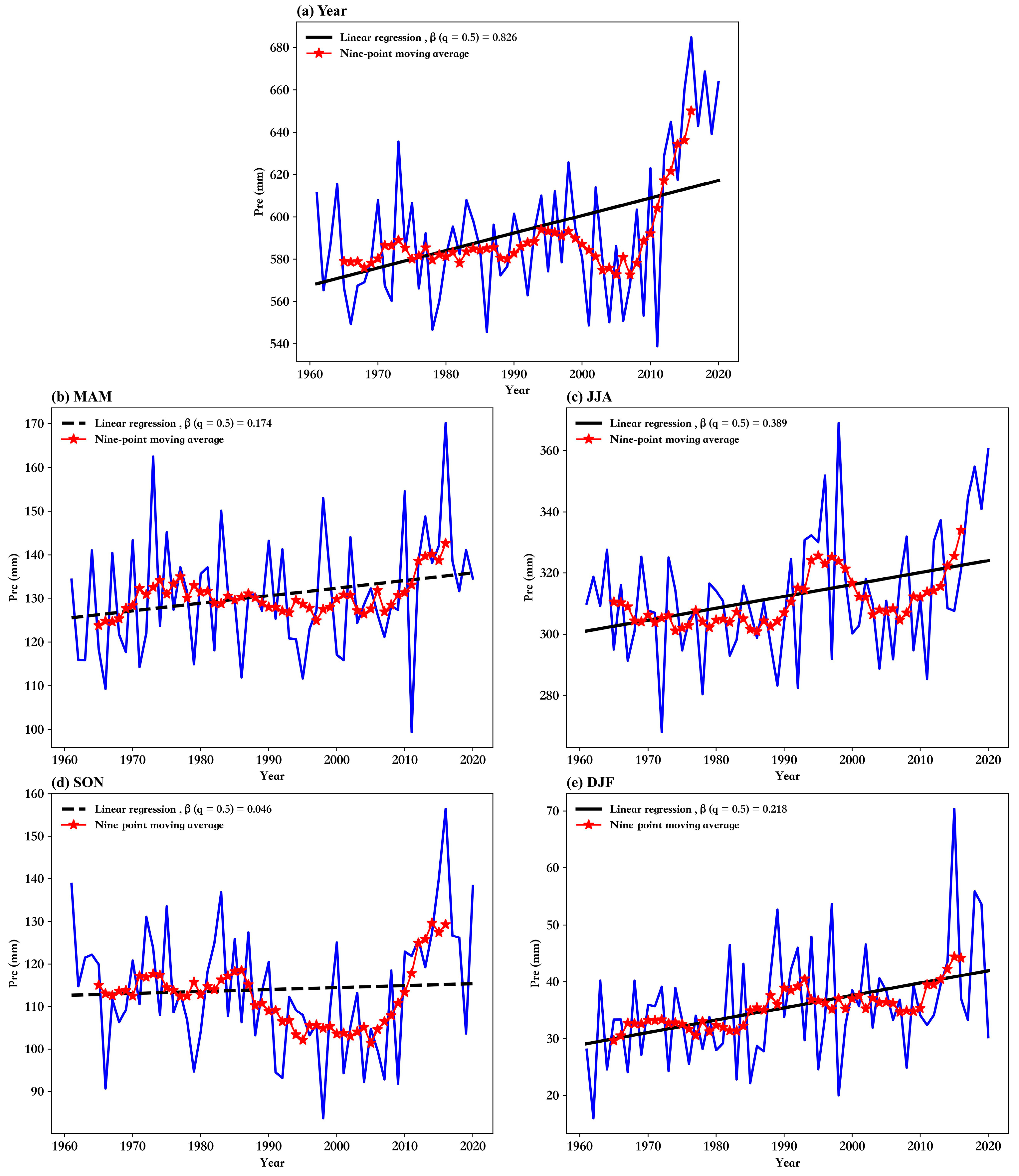
3.1. Annual and Seasonal Changes

To obtain a whole view of the precipitation in China, the average annual precipitation and four average seasonal time series were investigated, which indicated the average total precipitation (Figure 1a the whole year and Figure 1b–e the four seasons). The black lines are the median regression trends, and the red lines are nine-point moving average trends. Except in MAM and SON, the precipitation showed a significant increasing trend, which was different from some existing research results [16,18]. The research pointed out the precipitation trends during the recent 50 years across China were imperceptible but that the regional and seasonal changes were significant. Combined with the results of the nine-point moving average, precipitation, whether in the whole year or in the four seasons, has obviously increased since 2005. That could be caused by obvious interannual characteristics of precipitation. Especially in SON, the precipitation in 1990–2020 first decreased and then increased, causing an overall weakening trend from 1961 to 2020. In detail, the slope coefficients β(0.5) of the whole year and four seasons were 0.83 mm/a, 0.17 mm/a, 0.39 mm/a, 0.05 mm/a and 0.22 mm/a. The significant increases were in the whole year, JJA and DJF. That is, there were no significant increases in the transition seasons.

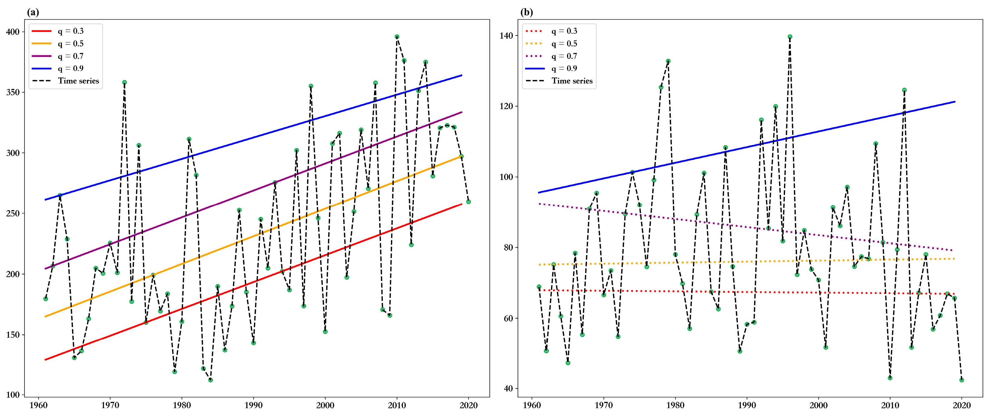
3.2. Quantiles Selection

Quantile regression was used to detect the trends of precipitation data in different parts. It could identify the homoscedasticity and heteroscedasticity of the data. If slope coefficient β(q) is constant for all quantiles, the variable is homoscedastic. If slope coefficient β(q) differs for different quantiles, the variable is heteroscedastic. Figure 2 is the result of the quantile regression of two representative grid precipitations. Trends in different quantiles were almost the same (Figure 2a), which indicated a homoscedastic relationship. In Figure 2b, trends in different parts varied, which indicated a heteroscedastic relationship. Solid lines indicated that the trends were significant, and the significance of trends in different quantiles of precipitation differed. In fact, most precipitation was heteroscedastic. Precipitation was observed data and was an interaction resulting from different nonlinear dynamic systems, which were complex. Thus, heteroscedasticity was the main characteristic of observed precipitation.
To obtain more details on the tendency, q = 0.1 ,   0.2 ,   ,   0.9 was calculated, corresponding to the 10 % ,   20 % , ,   90 % percentiles of precipitation. q = 0.5 is the quantile regression for the median and provides measures of central tendency. q = 0.1 ,   0.2 ,   0.3 ,   0.4 and q = 0.6 ,   0.7 ,   0.8 ,   0.9 regression values reflect the trends below/above the central level. Figure 3 gives the distribution of the slope coefficients of q = 0.1 ,   0.2 ,   0.3 ,   0.4 , separately, in JJA as an example. If the p-value of the regression coefficient of a given grid is less than 0.05, the grid has a significant trend at the 5% significance level and is labeled with a black dot. The following spatial distribution figures are labeled similarly, and we do not repeat them in this article. Below the median, positive trends of precipitation were found in mainly South China and the Tibetan Plateau. Negative trends were found in mainly North China and Xinjiang. The spatial characteristics of the regional distribution were similar in most areas of China, while there were differences in a few areas. Therefore, the sign consistency of each lattice point was considered. For q = 0.1 ,   0.2 ,   0.3 ,   0.4 , there were 16 categories with different signs. Table 1 shows the categories.
According to the classification by sign in Table 1, the involved sum was calculated statistically (Table 2). In the table, C was the classification, and PCT represented the number of grids in this classification as a percentage of the total number of grids. In Table 3, C and PCT have the same meanings. There were 60.4% grid points with the same symbols (both positive and both negative). Furthermore, because the 10th percentile ( q = 0.1 ) is a very small value and the involved data numbers were fewer, the trend in this quantile had more uncertainty. Then, the regression results of only q = 0.1 could be neglected. Therefore, the middle trends of q = 0.3 among q = 0.2 ,   0.3 ,   0.4   were chosen to represent situations below the median, which were defined as low precipitation.
A similar analysis was given in q = 0.6 ,   0.7 ,   0.8 ,   0.9 . The spatial distributions of the slope coefficients in JJA are shown in Figure 4. In the high percentiles, positive trend regions were more extensive than they were in the low percentiles. Moreover, the trends of annual precipitation in Northeast China had phase changes, from negative trends to positive ones. In other words, the annual precipitation increased over time in the northeast in JJA in high quantiles. Thus, this area deserves more attention. In the middle and lower reaches of the Yangtze River, the high-percentile precipitation increased significantly. This means that there was an increasing number of flood years in this region. Overall, regions with precipitation increases expanded gradually with the increase in quantiles. Similarly, sign consistency was calculated with Table 1, but q = 0.6 ,   0.7 ,   0.8 ,   0.9 . The statistical results are shown in Table 3. Nearly 62% of the grid points maintained sign consistency. The higher the quantile is, the more obvious the characteristics of precipitation regions are, and precipitation events over the 90th percentile are flood years. Therefore, flood years were considered individually. q = 0.8 can be regarded as a transitional period; then, with q = 0.6 ,   0.7 , sign consistency is maintained in more than 80% of the grid points. Hence, the q = 0.7 results indicate high precipitation, and the q = 0.9 results indicate flood precipitation.

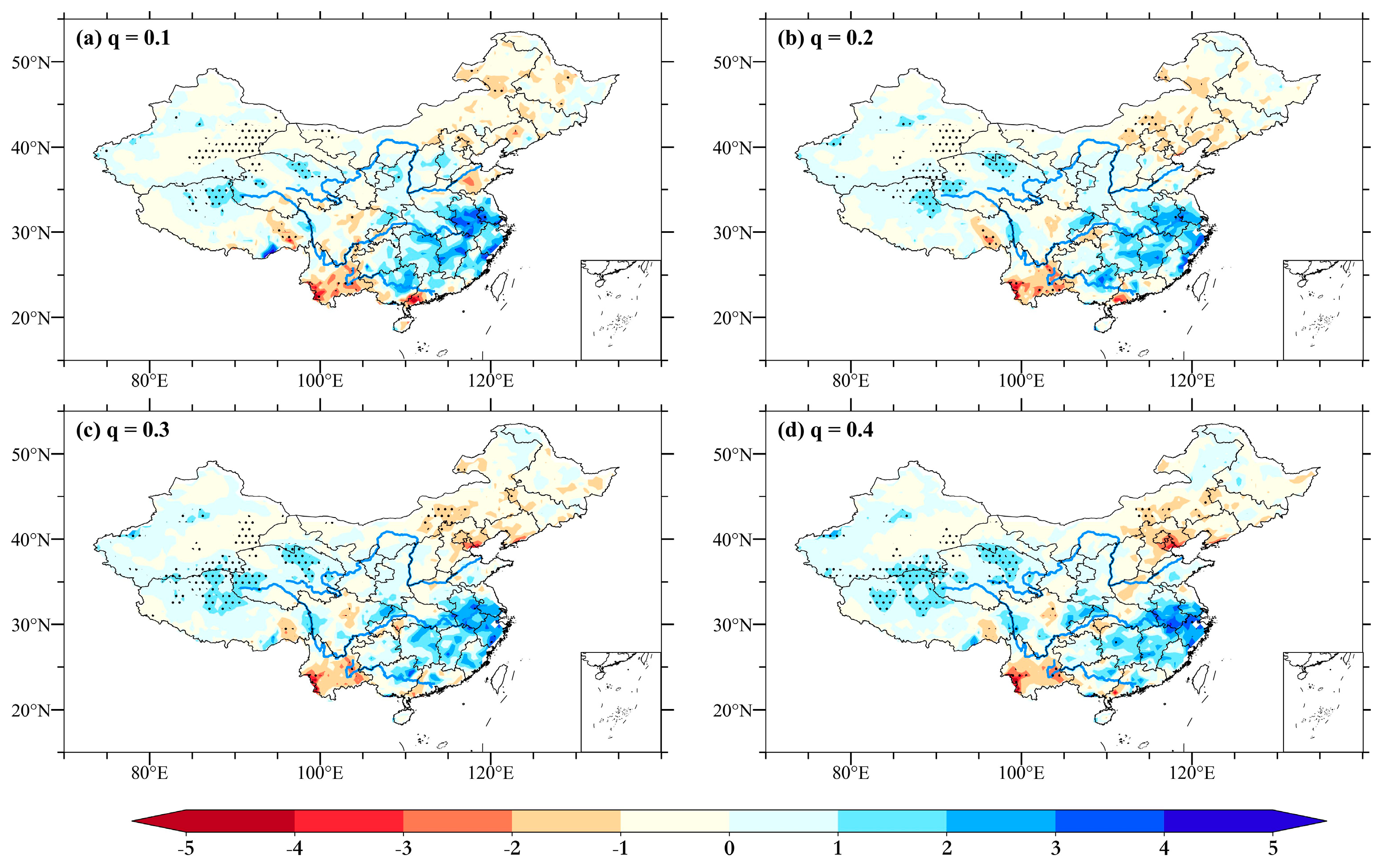
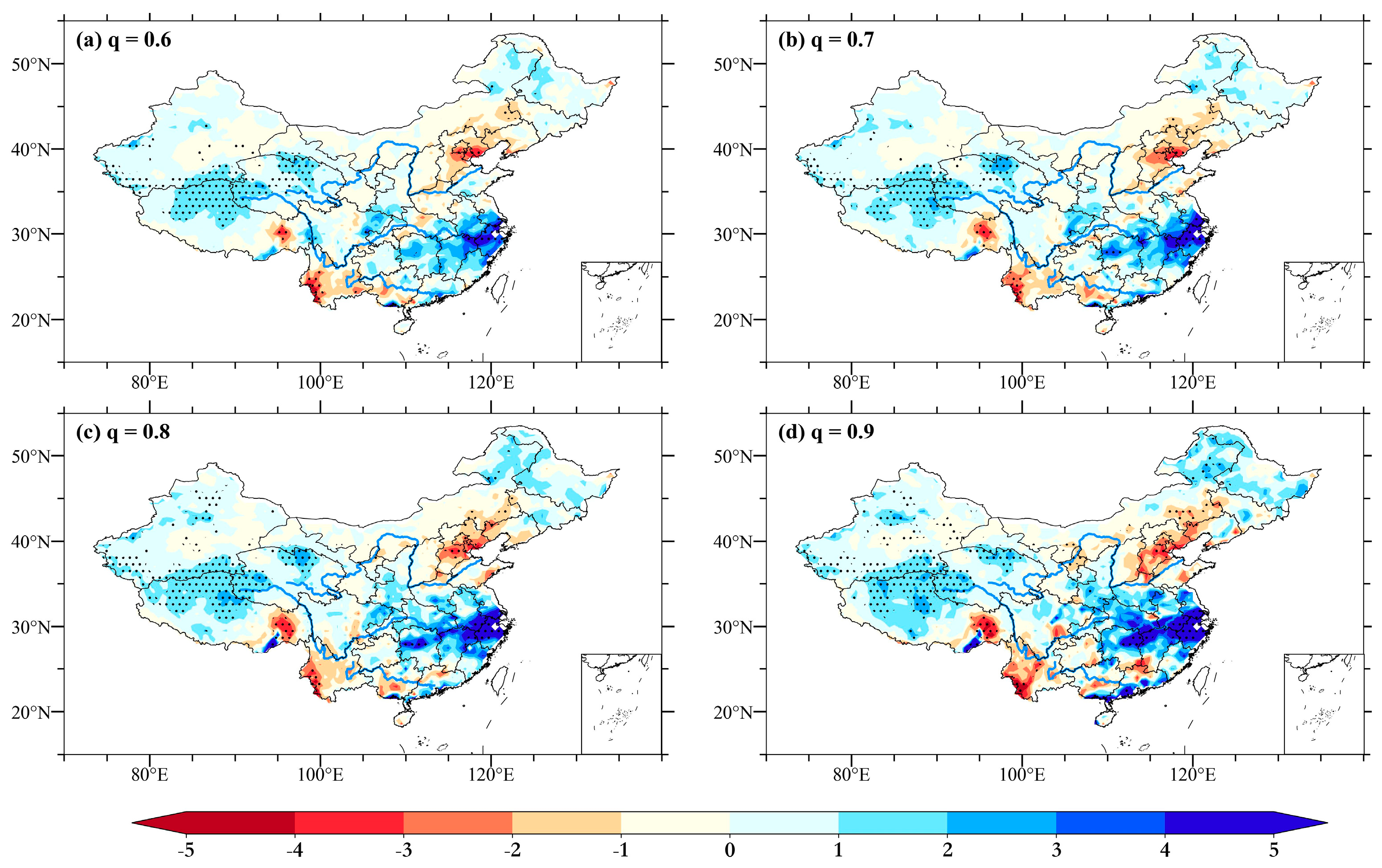
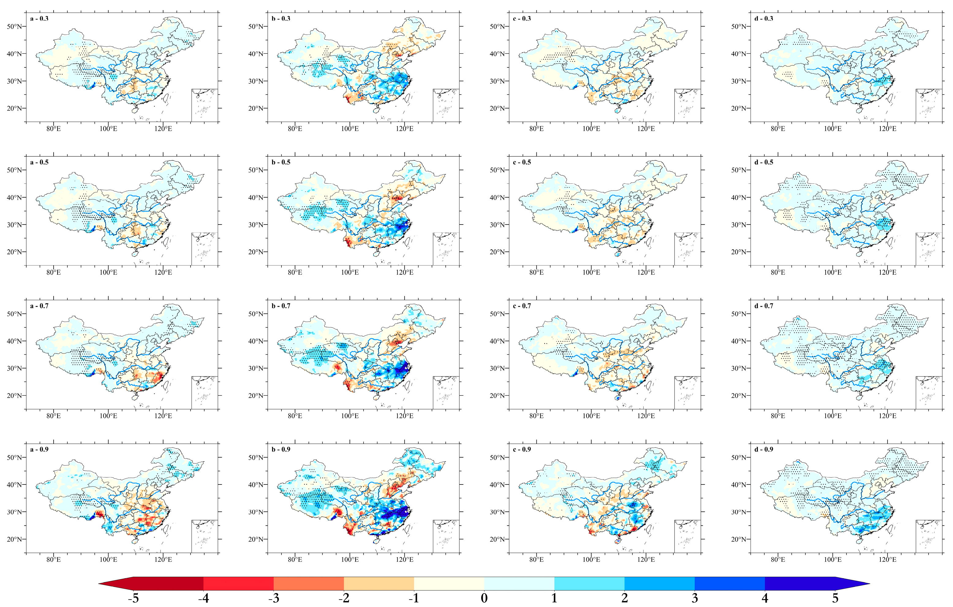
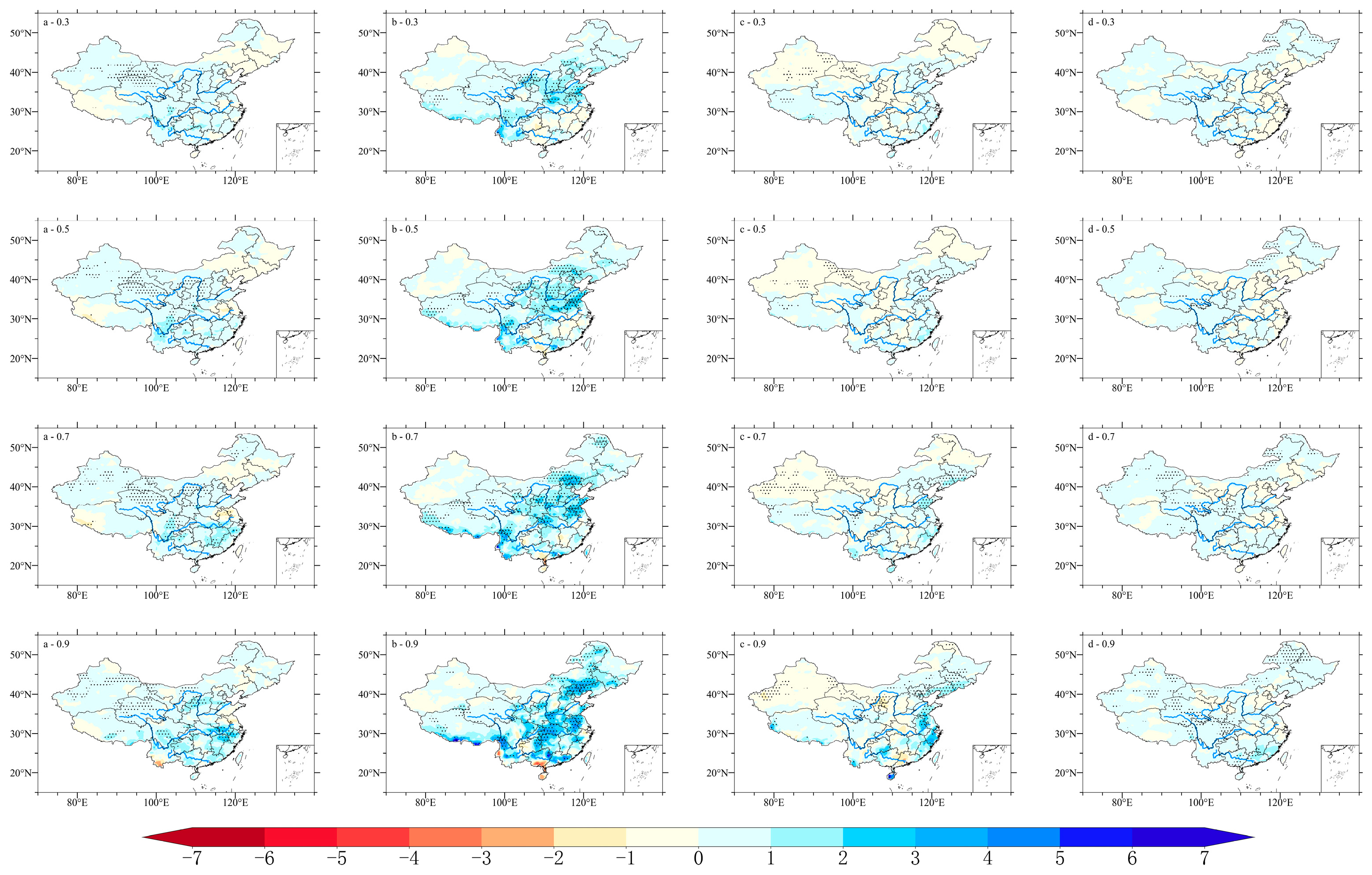
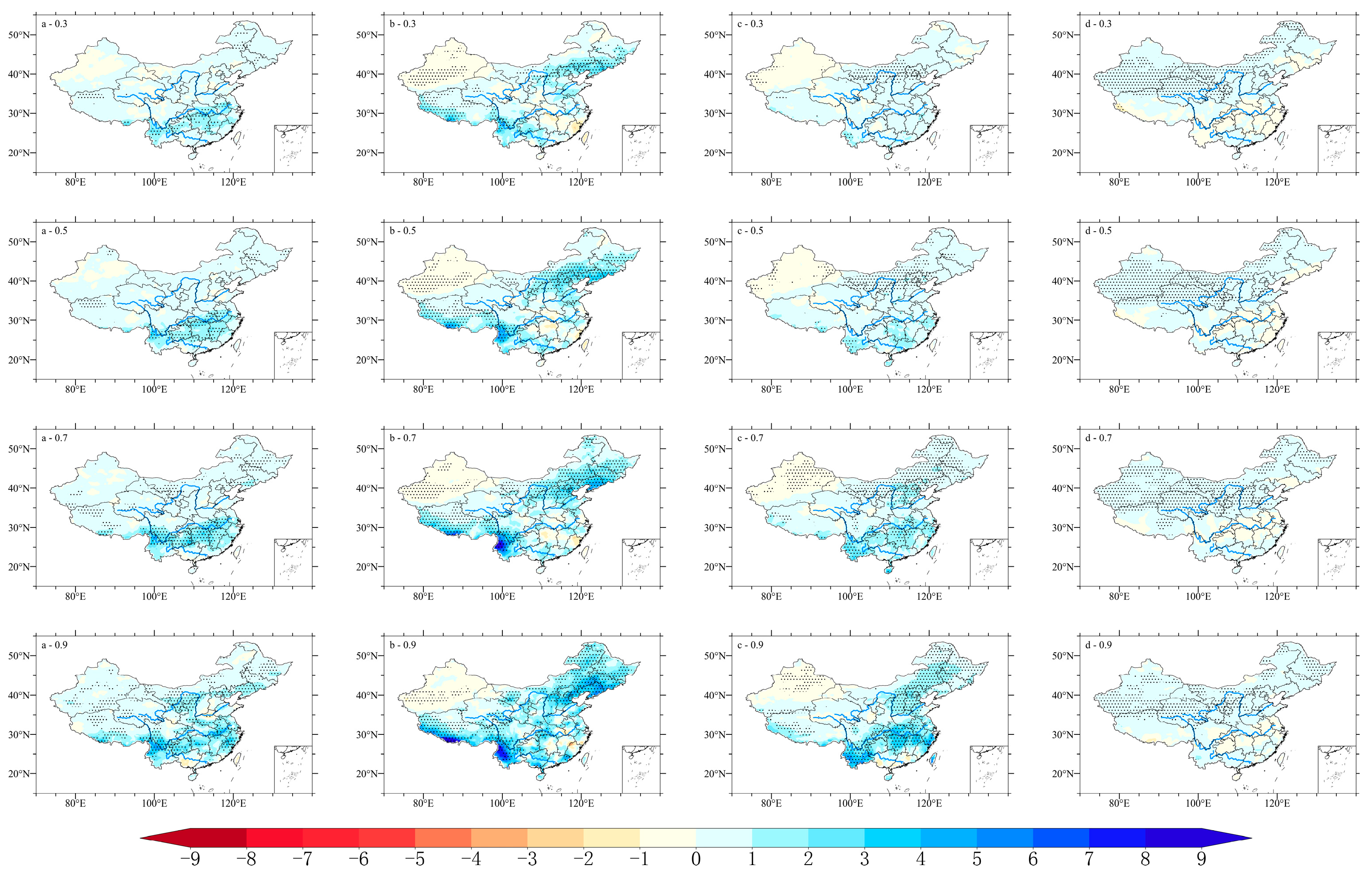
3.3. Different Trends Responses with Chosen Quantiles

If annual precipitation changes in every season over time, does it equally affect all the percentile values? Figure 5 shows the spatial trend distribution of precipitation over time in different seasons and attempts to answer this question. In most regions, the slope coefficients were similar in low, median and high precipitation, which reflected that precipitation changed similarly in different quantiles. Although the value of the slope coefficient in each grid was not exactly unchanged, the precipitation trend was considered similar within permissible limits. However, there were still sensitive regions that changed differently in low and high quantiles, especially in extremely high quantiles q = 0.9 .
In MAM, the slope coefficients changed in the interval [−6.65, 8.66] mm/year. Precipitation increased significantly in Northeast China. As the quantile increased, the trend became more obvious. Precipitation significantly decreased mainly in the western desert regions. However, in the middle and lower Yangtze Plains, precipitation showed a weak increasing trend in the low and median quantiles and an obvious decreasing trend in the high quantile, and the regions even extend to the North China Plain. That is, in the middle and lower Yangtze Plains, low and median precipitation increased, while high and flood precipitation significantly decreased. There was an increasing number of low precipitation years and normal precipitation years. In JJA, quantile regression coefficients ranged from −9.91 to 13.56 mm/year. As mentioned above, in Heilongjiang Province and in northern Inner Mongolia, precipitation decreased in the low quantile, whereas in the high quantile, it increased, which indicated a completely opposite trend adjustment. In the middle and lower reaches of the Yangtze River, flood precipitation years increase. While in North China, precipitation showed a consistently decreasing trend in all percentiles. Yan et al. [37] also found that in most parts of North China, drought had intensified. That means that the intensified drought in North China is mainly in JJA and was reflected in all intensity levels of precipitation. In SON, the precipitation trend range was [−6.80, 7.71] mm/year, which was close to that in MAM. In most regions, the precipitation trends were weak, either increasing or decreasing in low, median and high quantiles. However, flood precipitation in SON in Fujian, Jiangxi, Anhui Province and Northeast China significantly increased. Those regions had weak deceasing trends in the low, median and high quantiles. In DJF, the precipitation range was smallest in the four seasons: [−2.00, 4.17] mm/year. In most regions of China, precipitation significantly increased. As the quantile increased, the regions of significant increase became increasingly larger. Flood precipitation obviously increased in South China.
According to a comparison of the spatial distribution of the four seasons, DJF had relatively good consistency in the different quantiles. In the northwest of China, precipitation in high percentile in all seasons increased to different degrees, especially in JJA and DJF, which was consistent with the analyzed result of Sui et al. [38]. In other seasons, there were sensitive regions that changed with opposite trends in low and high quantiles. In MAM, in the middle and lower Yangtze Plain, low precipitation increased, whereas high and flood precipitation decreased. In JJA in Heilongjiang Province and northern Inner Mongolia, low precipitation decreased, whereas high precipitation, especially flood precipitation, increased, which indicated a similar change trend in SON. Previous studies [39,40] have also pointed out that in these regions, the intensity of annual precipitation increased, but the number of rainy days has decreased. In SON, in Fujian, Jiangxi and Anhui Province, flood precipitation obviously increased. These regions require more research attention, especially in regions with increases in high and flood precipitation.

3.4. Responses to Different Climate Changes Scenarios

To determine how annual precipitation is reflected in different percentiles in future climate change conditions, precipitation data from 2015 to 2100 from China Model BCC-CSM2-MR of scenarios SSP2-4.5 and SSP5-8.5 were analyzed. Figure 6 and Figure 7 show the analyzed SSP2-4.5 and SSP5-8.5 results in the four seasons. In general, the precipitation in future climate change compared with observation data obviously increased in most regions, especially in the high radiative forcing scenario, and the annual and seasonal precipitation significantly increased at the 5% level. Table 4 gives the median trends in the SSP2-4.5 and SSP5-8.5 scenarios.
In the SSP2-4.5 scenario, precipitation increased mainly in MAM and JJA (Figure 6). In MAM, the low and median slope coefficients had similar spatial distributions. Except for Northeast China and central Inner Mongolia, most regions had increasing trends. Especially in the middle and lower Yangtze Plain, precipitation increased in all percentiles, and even flood precipitation significantly increased, which was the opposite of the observation results. In JJA, precipitation increased nearly everywhere, although in the middle and lower reaches, the Yangtze River precipitation had a weak decreasing trend only in the low and median percentiles. In northern China, precipitation more obviously increased with increasing quantiles. There was no opposite trend adjustment with the observation results. In SON, although the overall trend was increasing, the precipitation in Xinjiang still had an obvious decreasing trend in all percentiles. As a vulnerable ecological area, Xinjiang in the middle radiative forcing scenario deserves more attention. At the same time, the flood precipitation in Northeast China significantly increased, whereas the low, median and high precipitations had opposite trends. According to regional sensitivity, SON was more repressed. In DJF, except for the flood precipitation significantly increasing, the low, median and high precipitations weakly increased.
Compared with the SSP2-4.5 scenario, with the high radiative forcing scenario, precipitation increased more. Basically, precipitation significantly increased in every season in most regions, and the increases were similar in different percentiles. Only Xinjiang in JJA and SON still had significantly decreasing trends, especially in JJA, which was the opposite of the result of the SSP2-4.5 scenario. Combining these two scenarios with observation results, heteroscedasticity was more evident in the actual observed precipitation data. That is, in future climate change, the precipitation changed similarly in different percentiles. In the high radiative forcing scenario, homoscedasticity was more obvious.

4. Conclusions

With global warming, previous studies have found nonuniform responses of precipitation because of regional differences. Precipitation has increased in some areas and decreased in others, and these studies have focused mainly on changes around the mean or extreme values. In fact, precipitation observation data are the result of mutiscale nonlinear complex systems, and the precipitation data on China are affected by complex climatic and natural geographical conditions and climate change effects in the whole precipitation data structure. That is, significant responses of precipitation to climate change may represent different parts of precipitation. Thus, does some part of the precipitation have a significant response to climate change? If yes, do the significant responses have regional characteristics? Here, we used quantile regression to reflect the trend of every part of the data to detect different parts of precipitation changes in China.
For the observation data, all the analyzed results of precipitation in the median percentile showed that the average annual, JJA and DJF had significant increases, whereas the increasing trends in MAM were weak. In general, precipitation in China increased significantly under the background of global warming, and the increase was mainly represented in JJA, followed by DJF. The nine-point moving average trends showed that the increase obviously began in approximately 2005, which is why previous research in China did not show an increasing response, because the analyzed precipitation time series were not up to date. This result also reflects the obvious interannual characteristics of the precipitation data. Quantiles q = 0.1, 0.2, ⋯, 0.9 were analyzed to obtain more details on different parts of precipitation. On the basis of the sign consistency of the slope coefficients with quantile regression, the results of quantiles q = 0.3, 0.5, 0.7, 0.9 were selected to represent low, median, high and flood precipitation. Each of the four seasons was separately analyzed to determine the seasonal characteristics of precipitation in China. Precipitation data showed that the trend was consistent in different parts of precipitation in most regions in China, i.e., the increasing or decreasing trend remained the same in every quantile, but the increasing or decreasing trend was more obvious as the quantile increased. However, in every season, there were some sensitive regions with abnormal responses to low and high precipitation. These regions deserve more attention, especially for agriculture managers. In MAM, in the middle and lower Yangtze Plains, the low and median precipitation increased, whereas the high and flood precipitation significantly decreased. There were increasing numbers of low precipitation years and normal precipitation years. In JJA, Heilongjiang Province and northern Inner Mongolia had decreasing trends in the low quantile and increasing trends in the high quantile, indicating a completely opposite trend adjustment. In the middle and lower reaches of the Yangtze River, the number of flood precipitation years increased. In SON, flood precipitation in Fujian, Jiangxi, Anhui Province and Northeast China significantly increased. In DJF, flood precipitation obviously increased in South China. Precipitation with obviously different responses in the low and high percentiles was present mainly in MAM and JJA.
To compare the observation results, the precipitation levels from two future climate change scenarios, SSP2-4.5 and SSP5-8.5, were analyzed. Precipitation in future climate change will increase with increasing radiative forcing. Thus, heteroscedasticity was not as evident compared with practical observation data.
Precipitation is a synergistic result of different spatiotemporal nonlinear systems, and understanding its dynamics and mechanisms is a complex and long-term process. Here, only the heteroscedasticity characteristics of precipitation over time were briefly analyzed. Future research questions include the following: How do the interdecadal changes over time affect the heteroscedasticity of precipitation events? How do extra-forcing signals affect the precipitation heteroscedasticity? These are research questions we will continue to address.

Author Contributions

Z.Q. contributed to conception and design of the study. L.W., X.C., H.Z. and Z.L. organized the database. Z.Q. and L.W. wrote the first draft of the manuscript. All authors have read and agreed to the published version of the manuscript.

Funding

This research was funded by the National Natural Science Foundation of China (Grant Nos. 41975062, 41675050).

Institutional Review Board Statement

Not applicable.

Informed Consent Statement

Not applicable.

Data Availability Statement

This study data was provided by Climate Data Center of the China National Meteorological Administration.

Conflicts of Interest

The authors declare no conflict of interest.

References

  1. Rana, A.; Uvo, C.B.; Bengtsson, L.; Sarthi, P. Trend analysis for rainfall in Delhi and Mumbai, India. Clim. Dyn. 2011, 38, 45–56. [Google Scholar] [CrossRef]
  2. Higham, J.; Cohen, S.A.; Cavaliere, C.T.; Reis, A.; Finkler, W. Climate change, tourist air travel and radical emissions reduction. J. Clean. Prod. 2016, 111, 336–347. [Google Scholar] [CrossRef] [Green Version]
  3. Chen, Z.Y.; Cai, J.; Gao, B.B. Detecting the causality influence of individual meteorological factors on local PM2.5 concentration in the Jing-Jin-Ji region. Sci. Rep. 2017, 7, 407352. [Google Scholar] [CrossRef] [PubMed] [Green Version]
  4. Tobin, K.J.; Bennett, M.E. Adjusting satellite precipitation data to facilitate hydrologic modeling. J. Hydrometeorol. 2010, 11, 966–978. [Google Scholar] [CrossRef]
  5. Chatterjee, S.; Khan, A.; Akbari, H.; Wang, Y.P. Monotonic trends in spatio-temporal distribution and concentration of monsoon precipitation (1901–2002) West Bengal, India. Atmos. Res. 2016, 182, 54–75. [Google Scholar] [CrossRef]
  6. Wang, Y.F.; Xu, Y.F.; Lei, C.G. Spatio-temporal characteristics of precipitation and dryness/wetness in Yangtze River Delta, eastern China, during 1960–2012. Atmos. Res. 2016, 172, 196–205. [Google Scholar] [CrossRef]
  7. Ronghui, H.; Rongshuo, C.; Jilong, C.; Liantong, Z. Interdecadal Variations of Drought and Flooding Disasters in China and Their Association with the East Asian Climate System. Chin. J. Atmos. Sci. 2006, 30, 730–743. [Google Scholar]
  8. IPCC-Intergovernmental Panel on Climate Change. Climate Change 2014: Impacts, Adaptation, and Vulnerability; Cambridage University Press: Cambridage, UK, 2014. [Google Scholar]
  9. Onof, C.; Arnbjerg-Nielsen, K. Quantification of anticipated future changes in high resolution design rainfall for urban areas. Atmos. Res. 2009, 92, 350–363. [Google Scholar] [CrossRef]
  10. Quirmbach, M.; Einfalt, T.; Langstadtler, G. Climate change analysis of precipitation data for North Rhine-Westphalia. Atmos. Res. 2012, 109–110, 1–13. [Google Scholar] [CrossRef]
  11. Irannezhad, M.; Marttila, H.; Klove, B. Long-term variations and trends in precipitation in Finland. Int. J. Climatol. 2014, 34, 3139–3153. [Google Scholar] [CrossRef]
  12. Zhao, J.; Feng, G.; Yang, J. Analysis of the distribution of the large-scale drought/flood of summer in China under different types of the western Pacific subtropical high. Acta Meteorol. Sin. 2012, 70, 1021–1031. (In Chinese) [Google Scholar]
  13. He, B.; Zhai, P. Changes in persistent and non-persistent extreme precipitation in China from 1961 to 2016. Adv. Clim. Chang. Res. 2018, 9, 177–184. [Google Scholar] [CrossRef]
  14. He, J.; Wu, Z.; Jiang, Z. “Climate effect” of the northeast cold vortex and its influences on “Meiyu”. Chin. Sci. Bull. 2006, 51, 2803–2809. (In Chinese) [Google Scholar] [CrossRef]
  15. Shi, N.; Huang, X.; Yang, Y. Temporal and spatial characteristics of the trend of global precipitation annual precipitation field from 1948 to 2000 Chinese. Atmos. Sci. 2003, 27, 971–982. (In Chinese) [Google Scholar]
  16. Zhai, P.M.; Wang, C.; Li, W. A Review on Study of Change in Precipitation Extremes. Clim. Chang. Res. 2007, 144–148. (In Chinese) [Google Scholar]
  17. Liu, F.; Ouyang, Y.; Wang, B.; Yang, J.; Ling, J.; Hsu, P.C. Seasonal evolution of the intraseasonal variability of China summer precipitation. Clim. Dyn. 2020, 54, 4641–4655. [Google Scholar] [CrossRef]
  18. Zhai, P.; Zhang, X.; Wan, H.; Pan, X. Trends in total precipitation and frequency of daily precipitation extremes over China. J. Clim. 2005, 18, 1096–1107. [Google Scholar] [CrossRef]
  19. Wu, Y.; Guo, J.; Lin, H.; Bai, J.; Wang, X. Spatiotemporal patterns of future temperature and precipitation over China projects by PRECIS under RCPs. Atmos. Res. 2020, 249, 105303. [Google Scholar] [CrossRef]
  20. Jiang, Z.; Shen, Y.; Ma, T.; Zhai, P.; Fang, S. Changes of precipitation intensity spectra in different regions of mainland China during 1961–2006. J. Meteorol. Res. 2014, 28, 1085–1098. [Google Scholar] [CrossRef]
  21. Ren, G.; Ren, Y. Spatial and temporal patterns of precipitation variability over mainland China: II: Recent trends. Adv. Water Sci. 2015, 26, 451–465. (In Chinese) [Google Scholar]
  22. Li, W.; Zuo, J.; Song, Y. Change in Spatio-Temporal Distribution of Drought/Flood Disaster in Southern China Under Global Climate Warming. Meteorol. Mon. 2015, 41, 261–271. [Google Scholar]
  23. Liu, B.J.; Li, Y.; Chen, J.F.; Chen, X.H. Long-term change in precipitation structure over the karst area of southwest China. Int. J. Climatol. 2015, 36, 2417–2434. [Google Scholar] [CrossRef] [Green Version]
  24. Koenker, R.W.; Bassett, G. Regression quantiles. Econometrica 1978, 46, 33–50. [Google Scholar] [CrossRef]
  25. Yu, K.; Lu, Z.; Stander, J. Quantile regression: Applications and current research areas. Statistician 2003, 52, 331e350. [Google Scholar] [CrossRef]
  26. Chamaille-Jammes, S.; Fritz, H.; Murinadagomo, F. Detecting climate changes of concern in highly variable environments: Quantile regressions reveal that droughts worsen in Hwange national park, Zimbabwe. J. Arid Environ. 2007, 71, 321–326. [Google Scholar] [CrossRef]
  27. Barbosa, S.M. Quantile trends in Baltic Sea level. Geophys. Res. Lett. 2008, 35, L22704. [Google Scholar] [CrossRef]
  28. Luce, C.H.; Holden, Z.A. Declining annual streamflow distributions in the Pacific Northwest United States, 1948–2006. Geophys. Res. Lett. 2009, 36, L16401. [Google Scholar] [CrossRef] [Green Version]
  29. Timofeev, A.A.; Sterin, A.M. Using the quantile regression method to analyze changes in climate characteristics. Russ. Meteorol. Hydrol. 2010, 35, 27–41. [Google Scholar] [CrossRef]
  30. Liao, R.; Shen, Y.; Zhang, D.-B. Characteristics of winter rainfall in eastern China based on grid data. J. Meteorol. Environ. 2013, 29, 55–62. [Google Scholar]
  31. Eyring, V.; Bony, S.; Meehl, G.A.; Senior, C.A.; Stevens, B.; Stouffer, R.J.; Taylor, K.E. Overview of the CMIP6 experimental design and organization. Geosci. Model Dev. 2016, 9, 1937–1958. [Google Scholar] [CrossRef] [Green Version]
  32. Tareghian, R.; Rasmussen, P.F. Analysis of Arctic and Antarctic Sea ice extent using quantile regression. Int. J. Climatol. 2012, 33, 1079–1086. [Google Scholar] [CrossRef]
  33. Fan, L.; Xiong, Z. Using quantile regression to detect relationships between large-scale predictors and local precipitation over northern China. Adv. Atmos. Sci. 2015, 32, 541–552. [Google Scholar] [CrossRef]
  34. Tan, X.; Shao, D. Precipitation trends and teleconnections identified using quantile regressions over Xinjiang, China. Int. J. Climatol. 2017, 37, 1510–1525. [Google Scholar] [CrossRef]
  35. Bondell, H.D.; Reich, B.J.; Wang, H. Noncrossing quantile regression curve estimation. Biometrika 2010, 97, 825–838. [Google Scholar] [CrossRef] [Green Version]
  36. Koenker, R. Quantile Regression in R: A Vignette. 2006, Volume 13. Available online: http://www.econ.uiuc.edu/~roger/research/rq/vig.pdf (accessed on 1 September 2022).
  37. Yan, Z.; Yang, C. Geographic Patterns of Extreme Climate Change in China during 1951–1997. Clim. Environ. Res. 2000, 5, 267–272. (In Chinese) [Google Scholar]
  38. Sui, Y.; Jiang, D.B.; Tian, Z.P. Latest update of the climatology and changes in the seasonal distribution of precipitation over China. Theor. Appl. Climatol. 2013, 113, 599–610. [Google Scholar] [CrossRef]
  39. Trenberth, K.E.; Dai, A.; Rasmussen, R.M.; Parsons, D.B. The Changing Character of Precipitation. Bull. Am. Meteorol. Soc. 2010, 84, 1205–1217. [Google Scholar] [CrossRef]
  40. Jin, S.; Zhang, B.; Sun, L.; Ma, Z.; Zhao, Y.; He, X.Q. The Change Characteristics of Precipitation and Its Temporal Distribution Homogeneity in Hexi Region of China in Recent 50 Years. Resour. Sci. 2012, 34, 811–818. [Google Scholar]
Figure 1. Annual (a) and seasonal (be) changes in precipitation over time. The black lines are median regression trends. Red lines are nine-point moving average trends.
Atmosphere 13 02116 g001
Figure 2. Quantile regression of two representative grid precipitations: (a) Homoscedasticity; (b) Heteroscedasticity. The solid (light dash) line indicates the trend is significant (nonsignificant) at the 5% level.
Atmosphere 13 02116 g002
Figure 3. Distribution of slope coefficients in JJA with q = 0.1 ,   0.2 ,   0.3 ,   0.4 .
Atmosphere 13 02116 g003
Figure 4. Distribution of slope coefficients in JJA with q = 0.6 ,   0.7 ,   0.8 ,   0.9 .
Atmosphere 13 02116 g004
Figure 5. Spatial trends distribution of observation precipitation in MAM (a), JJA (b), SON (c) and DJF (d) with q = 0.3 ,   0.5 ,   0.7 ,   0.9 respectively.
Atmosphere 13 02116 g005
Figure 6. Spatial trends distribution of SSP2-4.5 precipitation in MAM (a), JJA (b), SON (c) and DJF (d) with q = 0.3 ,   0.5 ,   0.7 ,   0.9 , respectively.
Atmosphere 13 02116 g006
Figure 7. Spatial trends distribution of SSP5-8.5 precipitation in MAM (a), JJA (b), SON (c) and DJF (d) with q = 0.3 ,   0.5 ,   0.7 ,   0.9 , respectively.
Atmosphere 13 02116 g007
Table 1. Classification by sign of slope coefficients in different quantiles.
q   12345678910111213141516
0.1++++++++
0.2++++++++
0.3++++++++
0.4++++++++
Table 2. Sum of classifications by sign of slope coefficients with Table 1 in q = 0.1 ,   0.2 ,   0.3 ,   0.4 .
C12345678
SUM10571003596732540187
PCT27.63%2.61%0.92%2.51%1.91%0.65%1.05%4.89%
C910111213141516
SUM297644172217681981255
PCT7.76%1.67%1.07%1.88%5.67%1.78%5.19%32.81%
Table 3. Sum of classifications by sign of slope coefficients with Table 1 in q = 0.6 ,   0.7 ,   0.8 ,   0.9 .
C12345678
SUM14911938510960355694
PCT38.98%5.05%2.22%2.85%1.57%0.92%1.46%2.46%
C910111213141516
SUM19755246818086218874
PCT5.15%1.44%0.63%1.78%4.71%2.25%5.70%22.85%
Table 4. Precipitation median trends with different radiative forcing (mm/year).
AnnualMAMJJASONDJF
SSP2-4.50.96 *0.25 *0.57 *0.090.06
SSP5-8.51.75 *0.43 *0.77 *0.43 *0.12 *
Those with significant trends at the 5% level are marked with symbol *.
Publisher’s Note: MDPI stays neutral with regard to jurisdictional claims in published maps and institutional affiliations.

