Article

Numerical Simulation of Atmospheric Boundary Layer Turbulence in a Wind Tunnel Based on a Hybrid Method

1
School of Civil Engineering and Architecture, Northeast Electric Power University, Jilin 132012, China
2
Key Lab of Electric Power Infrastructure Safety Assessment and Disaster Prevention of Jilin Province, Northeast Electric Power University, Jilin 132012, China
3
Shaoguan Power Supply Bureau of Guangdong Power Grid O., Ltd., Shaoguan 512000, China
4
Northeast Electric Power Design Institute Co., Ltd. of China Power Engineering Consulting Group, Changchun 130021, China
5
Liaoning Provincial Transportation Planning & Design Institute Co., Ltd., Shenyang 110000, China
*
Author to whom correspondence should be addressed.
Atmosphere 2022, 13(12), 2044; https://doi.org/10.3390/atmos13122044
Submission received: 10 November 2022 / Revised: 23 November 2022 / Accepted: 5 December 2022 / Published: 6 December 2022
(This article belongs to the Special Issue Advances in Computational Wind Engineering and Wind Energy)

Abstract

:
In the Computational Fluid Dynamics (CFD) simulation for building structures, it is important to generate a stable atmospheric boundary layer (ABL) flow field that meets the standards. In this paper, the wind profile, turbulence intensity, and wind velocity power spectrum in the target region of a numerical wind tunnel were accurately simulated by a hybrid method. With the numerical simulation software FLUENT, the hybrid simulation method was implemented. In the hybrid simulation method, the wind field was simulated by setting the roughness element in the upstream of the model, adding random disturbance, and setting the circulation surface. The influences of simulation parameters (such as roughness element and random number parameters) and FLUENT solution methods on the flow field results were studied. The results show that the influence range of the roughness element on turbulence intensity is approximately 6 times its physical height. The turbulence intensity is positively correlated with the standard deviation of random numbers and negatively correlated with the assignment height. Finally, the wind fields for different terrains satisfying the standards were obtained in numerical wind tunnels. A simulation of the wind pressure on an inflatable membrane structure was illustrated. The comparison between numerical and experimental results shows a good accordance, which indicates a desirable potential in practical application.

1. Introduction

Modern high-rise buildings, large-span roof structures, and large-span bridge structures are flexible and sensitive to wind excitation. Adequate estimation of the wind-induced responses should be fully considered in the structural design process. Due to the advantages of economic and satisfactory results [1,2,3], the Computational Fluid Dynamics (CFD)-based numerical simulation has become a highly potential method to evaluate the wind effects on large-span structures. A key issue of CFD simulation is to obtain an atmospheric boundary layer (ABL) that meets the requirements of codes and standards.
Currently, the common processing methods of turbulence models in CFD include Direct Numerical Simulation (DNS), Reynolds-averaged Navier-Stokes (RANS) and Large Eddy Simulation (LES) [4]. The simulation results of the DNS method are mostly accurate, but it demands an extremely high computational consumption and is rarely adopted. Different from RANS which mainly focuses on the mean flow field, LES can provide results on the transient characteristics of turbulence by solving directly for large eddies above the grid scale [5]. Thus, the LES has better accuracy in turbulence simulation [6,7] and has been widely used in the field of wind engineering [8,9,10,11]. For example, Hassan et al. [12] investigated the atmospheric flow and dispersion of traffic exhaust by LES. They provided data for estimating, planning, and implementing urban exposure reduction. Based on LES, Nayer et al. [13,14] introduced a method for studying the wind-induced response of inflatable membrane structures considering the fluid-structure interaction effect. Auvinen et al. [15] combined a high-resolution LiDAR dataset to study the urban boundary layer flow in a coastal city.
To obtain more accurate simulation results on structural dynamic wind effects, the simulation methods on generating fluctuating wind field characteristics has been further investigated. There are three main methods to generate inflow turbulence of ABL in LES studies: synthetic turbulence, precursor simulation, and recycling [16,17].
The synthetic turbulence method mainly combines the generated fluctuating velocity on the target mean velocity. The fluctuating velocities can be generated by: the spectral method [18,19], the digital filter method [20,21], the proper orthogonal decomposition reconstruction method [22,23], and the vortex method [24]. The benefit of synthetic turbulence method is that it can generate non-uniform turbulence, which is suitable for complex inlets. However, it is difficult to satisfy the Navier-Stokes equations, which means that the turbulence characteristics may distort in the computational domain.
The principle of the precursor simulation method is to set a driving domain in front of the main computational domain and generate the target turbulence as the inlet boundary condition. In general, there are two types of precursor simulation methods. The first type is the passive simulation method that replicates the roughness arrangements in a wind tunnel test with the spires and roughness elements [25]. Using a similar idea, Yoshie et al. [26] simulated an unsteady non-isothermal turbulent boundary layer by some extremely thin aluminum plates. Another type of precursor simulation method is the precursor database method. Different from the passive simulation method, the precursor database method records the wind flow time series data generated by the driving domain in a database. Thus, the generated wind flow data can be used multiple times for inlet boundary conditions. The section of wind flow simulation can also be omitted in future use [17]. With this method, Thordal et al. [27] presented standard CFD setup guidelines of the precursor database models suitable for industrial employment. To more accurately record the wind flow data, Pimont et al. [28] presented a technique for capturing the effects of a pressure-gradient force (PGF). However, the precursor simulation method can not directly control the properties of the generated flow field. Moreover, due to the complex shape of the spires in the driving domain, it often requires a large number of computational grids as well as computational time.
To save the computational consumptions, some scholars had proposed the recycling method which determines a circulation surface in the computational domain. When the generated wind flow reaches the circulation surface, it is redirected to the inlet of drive domain for circulation until it meets the requirements. The recycling method based on periodic boundary was first proposed by Spalart [29]. Then, based on the similarity theory of smooth flat plate turbulent boundary, Lund et al. [30] used the scaling function to adjust the velocity field in the downstream and reassign it to the upstream inlet boundary. Nozawa and Tamura [31] applied Lund’s methods [30] to the simulation of a rough turbulent boundary. Kataoka [32] simplified Lund’s method and proposed the pseudo-periodic boundary conditions of the inlet and circulation surface. Recently, Zhang et al. [33] added an appropriate source term to the momentum equation to replace the effects of roughness elements. They also used the recycling method to improve computational efficiency. To summarize, at present, there are many simulation methods for turbulent inlet wind velocity, but the calculation accuracy and efficiency are different.
In order to improve the calculation efficiency of numerical wind tunnel and the accuracy of turbulence simulation, we propose a simplified hybrid simulation method of the numerical wind tunnel based on the existing simulation methods of turbulent inlet. Firstly, structured grids were divided in the flow field region. Using the LES technique, combined with the roughness elements array, random disturbance technique, and circulation surface wind velocity reintroduction technique, the wind environments of standard terrains according to the Chinese National Standard (CNS) were generated. Subsequently, the unstructured grids were divided in the space around the building model, and CFD simplification was achieved by the internal and external grid fusion technique. Finally, the membrane structure model in the numerical wind tunnel was carried out by the proposed numerical simulation method. Compared with the results obtained from the wind tunnel test, the effectiveness of the simplified hybrid method in this paper was verified.

2. Hybrid Numerical Simulation Method

2.1. Simulation Target

According to the CNS (GB50009-2012) [34], the power law is used to describe the variation characteristics of mean wind velocity with height, as shown in Equation (1).
U i ( z ) = U 0 i z z 0 i α i
where U i ( z ) is the mean wind velocity of terrain i at z height, i = A, B, C, D, representing the terrain type. U 0 i is the mean wind velocity for terrain i at the reference height. z 0 i is the reference height of terrain i. α i is the roughness index of terrain i.
The turbulence intensity of the flow in the model area needs to satisfy by [34]:
I i ( z ) = I 0 i z z 0 i α i
where I i ( z ) is the turbulence intensity of terrain i at z height. I 0 i is the nominal turbulence intensity for terrain i.
The power spectrum of horizontal fluctuating can be described by the Von Karman spectrum [35]:
f S U ( z , f ) σ U 2 = 4 f ¯ 1 + 70.8 f ¯ 2 5 / 6
f ¯ = f L U ( z ) U ( z )
L U ( z ) = 100 ( z 30 ) 0.5
where f is the frequency of fluctuating wind velocity. S U ( z , f ) is the spectrum of fluctuating wind velocity at z height. σ U is the root mean square of the fluctuating wind velocity. L U ( z ) is the turbulence integral scale at z height. U ( z ) is the mean wind velocity at z height.
According to the CNS (GB50009-2012) [34], the atmospheric boundary layer parameters of the standard terrains are given in Table 1.

2.2. Simulation Strategy

Conventionally, to simulate the wind fields of different terrains, user-defined function (UDF) programming was used by many scholars to set a given standard wind profile at the entrance. However, the wind field is seriously dissipated due to the obstruction of the roughness elements, the calculation domain walls, and the flow field. Therefore, the wind profile and the turbulence intensity in the model region have a significant error compared with the entrance.
A pseudo-periodic boundary condition method was used to form a steady wind flow field [32]. The computational domain of the numerical simulation is divided into the inflow driving region and the model region. The wind flow first circulates in the inflow driving region through the pseudo-periodic boundary condition method. When the flow field is stable and meets the relevant statistical characteristics, it enters the model region for computational fluid dynamics transient numerical simulation. The wind flow circulation from the circulation surface to the inlet boundary was achieved by the UDF in the FLUENT software.
The prototype atmospheric boundary layer was scaled at a ratio of 1:100 to establish a numerical wind tunnel. In the inflow driving region, nine rows of roughness elements were uniformly and equally spaced in the along-wind direction of the calculation domain. Four rows of roughness elements were uniformly and equally spaced in the across-wind direction. Each roughness element occupied the same size position of 1 m × 1 m, the length and width of roughness elements were set to 0.4 m, and the height was 0.25 m. To stabilize the wind velocity profile, the distance between the last row of roughness elements and the exit should be 10 times greater than the height of roughness elements. The boundary conditions on both sides were set as periodic boundary conditions, which are theoretically infinite in width, so the across-wind width was set as the occupancy size of four roughness elements. It can be seen from Table 1 that the maximum boundary layer height is 550 m. Therefore, the dimension of the calculation domain is 16 m × 4 m × 5.5 m, and its blocking ratio is less than 3% (permissible blocking ratio) [36]. The calculation domain is shown in Figure 1. The x-direction, y-direction, and z-direction are along-wind, across-wind, and vertical wind, respectively.
Since the roughness element arrangement can only affect the flow field within a certain height range, the turbulence intensity of the flow field outside the height space affected by the roughness elements is increased by adding random interference numbers above the roughness element array [37]. The root mean square of the random interference number is set to be approximately equal to the root mean square of the fluctuating wind velocity. In addition, the random interference numbers satisfy the 3σ criterion of the normal distribution [38] and the average value is 0, as shown in Figure 2. Therefore, the standard deviation of the random interference number approximately equals the root mean square of the fluctuating wind velocity, and it can be defined as [37]:
r a n d s t d ( I f i n a l I 0 ) × U ¯
where r a n d s t d is the standard deviation of random interference number added for a certain position. I f i n a l is the target turbulence intensity. I 0 is the turbulence intensity under the action of only roughness elements. U ¯ is the along-wind mean velocity.
Combining the pseudo-periodic boundary conditions, the inlet wind velocities of the wind flow field considering random interference effect can be expressed by the following [32]:
u i n l e t y , z , t = u ¯ i n l e t z + u r e c y y , z , t u ¯ r e c y y , z + ψ θ × r a n d s t d v i n l e t y , z , t = v r e c y y , z , t + r a n d s t d w i n l e t y , z , t = w r e c y y , z , t + ψ θ × r a n d s t d
where u y , z , t , v y , z , t , and w y , z , t represent the instantaneous wind velocity in along-wind, across-wind, and vertical directions, respectively. u ¯ y , z , v ¯ y , z , and w ¯ y , z are mean velocity in along-wind, across-wind, and vertical directions, respectively. The subscripts ‘inlet’ and ‘recy’ indicate the inlet and the circulation surface, respectively. ψ θ is the weight function, which is given by Equation (8).
ψ θ = 1 2 1 tanh 8 ( θ 1.0 ) 0.7 0.4 ( θ 0.3 ) / tanh ( 8 )
where θ = y/Ly, Ly is the thickness of boundary layer (vertical height of the calculation domain). The weight function ψ (θ) ≤ 1.0, which serves to improve the stability of calculation and reduces the fluctuation of the boundary layer cycling.

3. Simulation Setups

The main work of this section is to establish a numerical wind field model and use the LES method to obtain the wind field that meets the requirements by properly allocating the roughness element height and random number assignment method.

3.1. Calculation Domain and Grids

With the ICEM software, structured grids were used for grid generation of the flow field. The grids were divided uniformly in the x-direction and widened gradually after the last row of roughness elements with the grids in the y-direction kept the same as far as possible, and the grids near the roughness elements encrypted by exponential growth in the z-direction. The calculation domain after gridding is shown in Figure 3.
Two grid size levels were generated to study the influence of the grid number on the calculation results. Grid settings are shown in Table 2.

3.2. Boundary Conditions and Solution Settings

After meshing, the model was imported into FLUENT, and the boundary conditions were set as shown in Table 3. At the entrance of the calculation domain, the standard terrain exponential rate wind profile was added via UDF. Subsequently, the wind field of terrain B was illustrated, the reference height was 10 m, and the wind velocity at the reference height was 14.8 m/s. The converted reference height was 0.1 m, and the corresponding wind velocity was 7.42 m/s. The random disturbances in along-wind, across-wind, and vertical directions were added at a certain height above the roughness elements. The parameters of the random interference number are shown in Figure 4.

4. Parametric Analysis

In this section, the influences of roughness element height, random number assignment methods (size, height, direction), and FLUENT solution methods on the flow field were studied as an example of terrain B. The atmospheric boundary layers of four standard terrains were simulated in the numerical wind tunnels, and the recommended values of the simulation parameters were given.

4.1. Effect of Grid Number

According to the principle of turbulence generation, the number of grids generally does not affect the mean wind velocity and turbulence intensity profiles but may affect the wind velocity power spectrum. Figure 5 shows the comparison between the power spectrum of simulation results and the target spectrum of two grid division schemes. The roughness element height in the simulation was 0.25 m, the standard deviation of the random number in the downwind direction was 1.393, and the assignment height of the random number was 1.3 m. The coordinate of the wind velocity measuring point was x = 14 m, y = 0.3 m, and z = 2 m. It can be seen from Figure 5 that Scheme 1 is significantly better than Scheme 2 in the 0.1-1 Hz frequency band in the power spectrum density chart. In Figure 5b, the high-frequency part of the wind velocity power spectrum is obviously smaller than the target spectrum. This is because the low-frequency part of the energy represents the energy of vortex larger than the grid scale, and the high-frequency part of the energy represents the energy of the vortex smaller than the grid scale. The LES takes the vortex larger than the grid scale as the main simulation object, and the simulation for the small vortex is insufficiently precise. Therefore, when the grid scale is small, the simulation of the large-scale vortex is more accurate. Considering that Scheme 1 has been able to simulate the vortex within 1 Hz accurately, the grid scale of Scheme 1 was used for modelling and analysis in the following studies.

4.2. Suggestion for Building Model Position

After the wind flows through the roughness region, the wind field will not be stable immediately. Therefore, it is necessary to determine the optimal position of the model by comparing the wind profiles of different x-direction positions. The calculation conditions for roughness elements and random interference numbers were the same as in Section 4.1. On the central axis of the y-axis in the calculation domain, six positions were selected along the positive direction of the x-axis (x coordinates are 10 m, 12 m, 13 m, 12.5 m, 14 m, and 15 m, respectively.). Forty-five points were selected as wind velocity monitor points for each position with equal height, whose starting height and interval were 0.075 m. The wind velocity and turbulence intensity profiles at different x positions of the model region are shown in Figure 6. When the vertical height is lower than 1.5 m, the change in position of the wind profile monitoring point along the x-axis has little effect on the mean wind velocity profile but has a significant effect on the turbulence. Within a vertical height of 1.5 m, the mean turbulence intensity error for each measurement point is at x = 10 m, 12 m, and 13 m is 21.9%, 13.7%, and 12.4%, respectively. The mean turbulence intensity error for each measurement point is at x = 10 m, 12 m, and 13 m is 6.4%, 5.6%, and 5.7%, respectively. As a result, the turbulence tends to be stable when x ≥ 13.5 m. The building model is suggested to be set between the positions among 13.5 m and 15 m in the x-axis direction.

4.3. The Influence of the Radom Number Parameters

From the above, the stable region of the wind field was after 13.5 m, so the simulation data in this paper were monitored and extracted at x = 14 m, y = 2 m, and z = 2 m. The influences of the normal distribution range, standard deviation, assignment direction, and assignment height of random numbers on the simulation results were studied and the law was summarized, laying the foundation for the simulation of a standard flow field. The working conditions of random number studies are shown in Table 4.
Because the random number added at the inlet and the root mean square of the fluctuating wind velocity extracted from the circulation surface and superimposed on the inlet are both 0, the method of assigning random numbers does not affect the mean wind velocity profile. Only the simulation results of the turbulence intensity profile are compared here.
Figure 7 shows the effect of random number parameters on turbulence intensity. Figure 7a shows that the range of values taken by the normal distribution has no effect on the turbulence intensity profile. In other words, since most of the probability values of the normal distribution are within (−1.5σ, 1.5σ), the probability of getting out of this area is not high. However, the larger the range of values, the more they can reflect the random process, so this paper chooses the normal distribution in the (−3σ, 3σ) to simulate. As can be seen from Figure 7b,c, the standard deviation of random numbers is positively correlated with turbulence intensity. If no roughness elements are added and random numbers are added above 0.25 m, the upper flow profile can be maintained. However, the lower turbulence intensity is too large, and the profile shape cannot be maintained. Therefore, only assigning random numbers cannot achieve the results of simulating standard terrains. When roughness elements and random numbers are both added, the turbulence intensity profile of the upper flow field is close to the referred standard, and the change is minimal compared with that without the roughness elements. In the vertical height range of 1.5 m, the turbulence intensity profile changes obviously compared with that without roughness elements, and it is also close to the reference standard. It shows that the influence height of the roughness element on turbulence intensity is about 6 times its height. The turbulence can reach the reference standard only by adding roughness elements in the lower flow field. But the upstream flow field needs to be stable. To fulfil this requirement, the standard deviation of random numbers are adjusted. As is seen in Figure 7d, the simulation results of adding random numbers in different directions are quite different. However, the shape of the turbulence profile can be maintained in all three conditions. It shows that it is feasible to change the assignment direction of random numbers to influence the turbulence intensity. The influence degree on the flow is that the along-wind direction is greater than the across-wind direction and greater than the vertical direction. Figure 7e shows the turbulence intensity profiles from the flow field of different random number assignment heights. With the increase in height, changing the assignment height of random numbers has little effect on the upper flow field but greatly influences the lower flow field. The lower the assignment height, the greater the turbulence intensity and the steeper the turbulence profile. Therefore, for the simulation of different terrains, it is necessary to find a suitable assignment height for random numbers.

4.4. The Influence of Solution Methods

There are many combinations of solution methods in FLUENT software, including first-order upwind, second-order upwind, and bounded central difference. Because each solution method may influence the simulation results differently, we analyzed four solution methods that may affect the calculation results. The cases of analysis are shown in Table 5.
The simulation results of different solution methods are displaced in Figure 8. It can be seen that the methods of first-order upwind and increasing the dissipative part velocity for solution are unsatisfactory in the region affected by the roughness elements. The mean wind velocity and turbulence intensity profiles simulated by the bounded center difference method are closer to the standard. Therefore, the control equation was solved by LES simulation and discretized by the SIMPLE algorithm and Standard format. The bounded central difference was used to discretize momentum and sub-grid scale kinetic energy. The turbulence model was bounded second-order implicit. The sub-grid stress model adopted the Kinetic-Energy Transport (KET) model. The time step was set as 0.015 s, and the maximum number of iterations was set as 10.

4.5. Recommendation Simulation of Standard Terrains

According to the above analysis of random number parameters and roughness elements, the flow field was continuously adjusted, and finally, the numerical wind tunnels of common standard terrains were simulated. The numerical wind tunnels were established with a 1:100 scale ratio. Table 6 shows the roughness element height and random number parameters for simulating various terrains.
Figure 9 depicts the comparison of the wind velocity and turbulence intensity profiles in the numerical wind tunnel and the targeted CNS. The simulation results of the mean wind velocity profile are very close to the standard. The simulation results of turbulence intensity in the lower part of wind fields of various terrains are slightly larger than the standard, mainly affected by roughness elements. Generally, the profiles are basically close to the standard, and the simulations are satisfactory.
The comparisons of power spectrums of fluctuating wind velocities for different terrains are shown in Figure 10. The simulations are consistent with the reference standard in the 0–0.9 Hz range. However, the power spectrum of high-frequency sag is a common phenomenon in numerical simulation. The high-frequency component of wind velocity still needs to be improved by refining the grid. Because the low-order modal response of general buildings can be excited, the simulation results are acceptable.

5. Engineering Application and Verification

In this section, the inflatable membrane structure with rectangular plane was taken as an illustration. The mean wind pressure coefficients obtained by LES and wind tunnel tests were compared to verify the feasibility and effectiveness of the numerical method.

5.1. Detials of Wind Tunnel Test and Numerical Simulation

The length (L), span (S), and height (H) of the inflatable membrane structure with rectangular plane are 120 m, 60 m, and 30 m, respectively. The shape of the membrane structure and definition of wind direction are illustrated in Figure 11. To keep the blocking rate less than 3%, the geometric scale ratio 1:100 was selected in the numerical simulation and wind tunnel test. The wind field of terrain B was simulated, and the wind velocity was 15 m/s.
Figure 12 shows the models in the wind tunnel test and numerical simulation. The tests were carried out in the wind tunnel at the Tianjin Research Institute for Water Transport Engineering. As shown in Figure 12a, the wind field of terrain B was simulated by arranging spires and roughness elements in the wind tunnel test. Based on the 3D printing technology, the model was made by SLA photosensitive resin material. Several stiffeners were arranged inside the model to ensure that the model had enough stiffness and strength for pressure tests under the wind load.
In the numerical simulation, considering that the flow field in the wake region of membrane structure is fully developed to prevent the backflow phenomenon from affecting the simulation results, the x-direction of the calculation domain was lengthened by 2 m. Therefore, the size of the calculation domain was x = 18 m, y = 4 m, z = 3.5 m. The membrane structure was placed at x = 14.2 m in the wind field stability region, and the distance between the outlet and the leeward side of the structure was greater than 9H (H is the height of the membrane structure). The calculation domain was divided into the flow field region and the model region, as shown in Figure 12b. To ensure accuracy and improve the calculation velocity, the flow field region adopted the structured grid, but the unstructured tetrahedral grid was adopted in model region. The structural model was placed in a cylindrical region with a radius of 1 m and a height of 0.5 m, and its grid growth rate was 1.2. The minimum grid size of the membrane structure surface was H/100, and that of the cylinder surface was 3H/200. The overall grid number is 24.7 million. The boundary conditions, solution settings, and random number parameters were consistent with the descriptions in Section 3 and Section 4.5.

5.2. Comparisons of Wind Tunnel Test and Numerical Simulation

To verify the simulation results, the results under three typical wind directions (0°, 30°, and 90°) were compared. Figure 13 shows the contours of the mean wind pressure coefficient under different wind directions. It can be observed that the experimental results show good agreement with the simulated results. Most structural regions are subject to negative wind pressure (suction), while the windward region is subject to positive wind pressure (pressure) from incoming wind loads. Compared with the wind tunnel test results, the positive pressure area at structural windward region in the numerical simulation is slightly smaller. This may be caused by errors in the structural curvature between the models of wind tunnel test and numerical simulation when modeling. At the flow separation corners, the wind pressure obtained by simulation is underestimated. This phenomenon had also been found in other studies [33,39,40]. There are many causes for this error, such as model errors, poor gridding, inappropriate turbulence models and solution methods, etc. To clarify the explanation for this error, further research is needed.
Taking 0° wind direction as an example, Figure 14 compares the wind pressure coefficients on the central axis with the previous study and wind tunnel test. It can be seen that the distribution of the wind pressure coefficients from numerical simulation is basically similar to the results of [41] and wind tunnel test. The values from numerical simulations are closer to those from wind tunnel tests. However, there is still a difference at the leeward area compared with the results of [41]. It may be caused by the different curvatures and shapes of the models. In the study of [41], the structural shape is semicylindrical. At the bottom of the leeward region, the numerical simulation results show positive values, while the results of [41] and wind tunnel test are negative. It indicates that the flow reattachment phenomenon occurs at the leeward region in the numerical simulation.
At 0° and 30° wind directions, the leeward region is subjected to the less positive pressure which is more obvious in the numerical simulation. To visually observe the flow around the structure in the wind field, Figure 15 depicts the instantaneous velocity contours with streamlines after the wind field is stabilized at 0° wind direction. As shown in Figure 15, because of structural blocking effect, the flow velocity drops sharply when it reaches the bottom at structural windward region. Then the flow velocity increases with the height of the structure, reaching a maximum at the top and creating a suction effect for the structure. Since the flow separation and reattachment phenomena, there are significant vortexes at the leeward region of the structure. The vortex acts on the structural surface and generates pressure. Therefore, the vortex motion can be well-simulated by LES.
Generally, the distributions and values of the mean wind pressure coefficients obtained by numerical simulation and wind tunnel test are close. Thus, it is proved that the numerical simulation of atmospheric boundary layer turbulence in a wind tunnel based on the hybrid method adopted in this paper is feasible.

6. Conclusions

This paper proposed a simplified hybrid simulation method of the numerical wind tunnel with a faster calculation based on the existing simulation methods of turbulent inlet. Through parametric analysis, the influences of roughness element, random number parameters (distribution range, standard deviation, height, direction), and FLUENT solution methods on the wind field characteristics were obtained. Consequently, the numerical wind fields conforming to the CNS were obtained. Finally, the numerical wind tunnel was applied to practical application, and the results were compared with the wind tunnel test results to verify the effectiveness of the proposed method. The main conclusions are drawn as follows:
(1)
Combined with the large eddy simulation technique, roughness elements array, random perturbation technique, circulation surface wind velocity reintroduction technique, and the internal and external grid fusion technique, the wind fields meeting the CNS terrains are generated in the numerical wind tunnels. The wind field simulation strategies are provided.
(2)
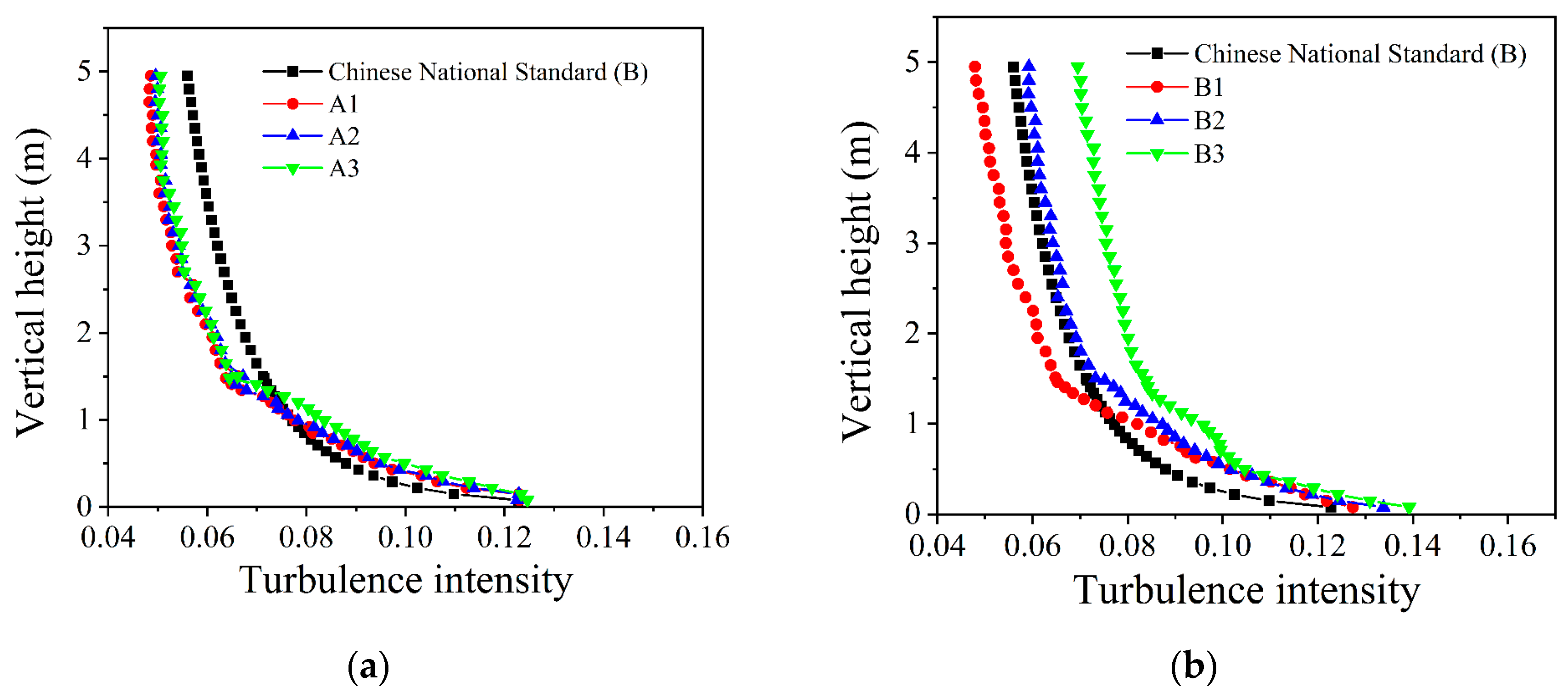
For random number assignment parameters, the normal distribution range does not typically affect the flow field, whereas the assignment direction has a significant effect. The free-stream turbulence intensity is positively correlated with the standard deviation of random number and negatively correlated with the assignment height. The influence height of the roughness element on turbulence intensity is about 6 times as high as its height.
(3)
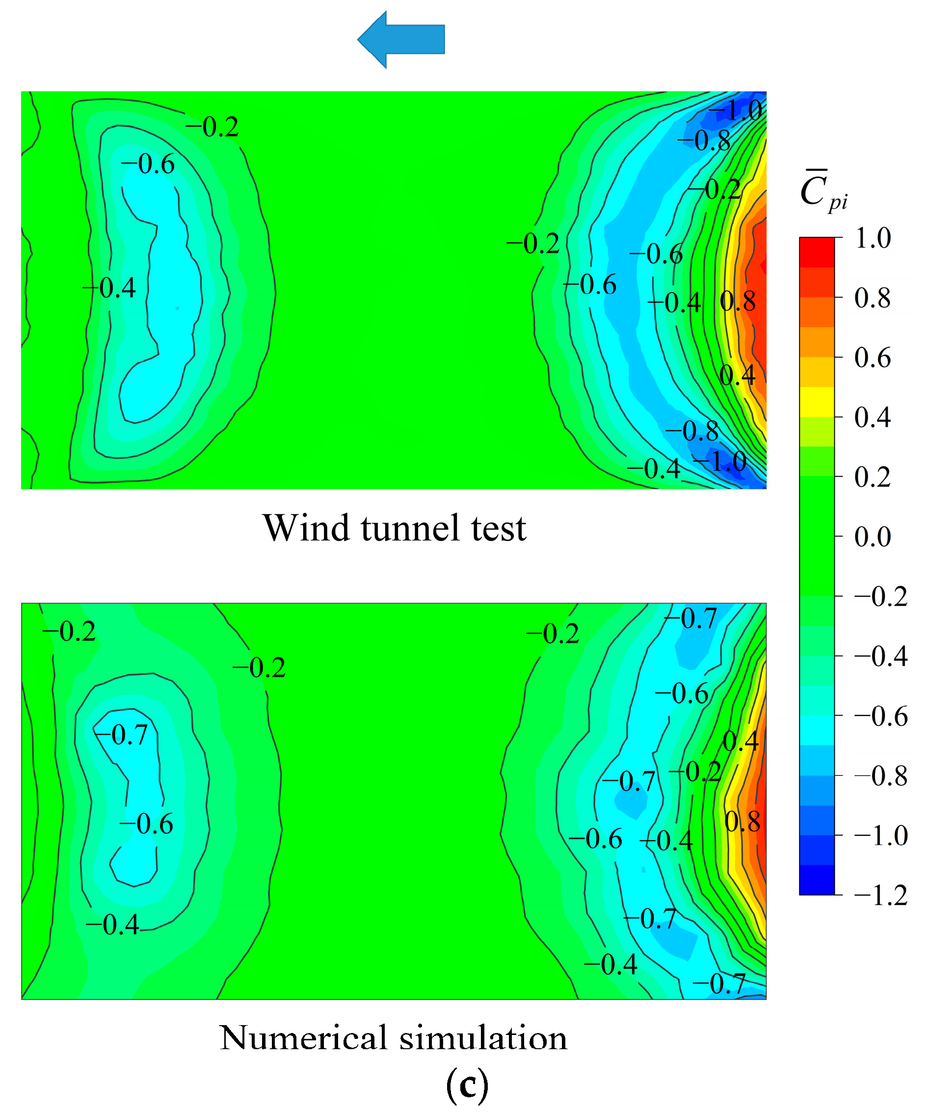
The effectiveness of the simulation method is validated by a practical engineering example of inflatable membrane structure in this paper. In terms of distribution and values, the wind pressure coefficients of inflatable membrane structure obtained from simulation show good agreement with the wind tunnel test. It is anticipated that the numerical wind tunnel simulation method proposed in this paper can be helpful for subsequent research.

Author Contributions

Conceptualization, Z.C. (Zhaoqing Chen) and L.T.; methodology, Z.C. (Zhuozhuo Chen) and C.W.; software, Z.C. (Zhuozhuo Chen), C.W. and S.W.; validation, Z.C. (Zhaoqing Chen) and L.T.; formal analysis, C.W. and S.W.; investigation, Z.C. (Zhuozhuo Chen); resources, Z.C. (Zhaoqing Chen); data curation, C.W. and Z.C. (Zhaoqing Chen); writing—original draft preparation, S.W. and C.W.; writing—review and editing, Z.C. (Zhaoqing Chen); visualization, L.T.; supervision, Z.C. (Zhaoqing Chen); project administration, Z.C. (Zhaoqing Chen); funding acquisition, Z.C. (Zhaoqing Chen). All authors have read and agreed to the published version of the manuscript.

Funding

The work described in this paper is grateful to the financial support of the National Natural Science Foundation of China (No. 51878129), the Supported by Foundation of Key Laboratory of Structures Dynamic Behavior and Control (Ministry of Education) in Harbin Institute of Technology (No. HITCE202004), and the Key Research and Development Plan of Jilin Science and Technology Department (20210203165SF).

Institutional Review Board Statement

Not applicable.

Informed Consent Statement

Not applicable.

Data Availability Statement

The data in this study are available on request from the authors.

Acknowledgments

The authors thank the anonymous referees for their valuable comments and suggestions.

Conflicts of Interest

The authors declare no conflict of interest.

References

  1. Kataoka, H.; Ono, Y.; Enoki, K. Applications and prospects of CFD for wind engineering fields. J. Wind Eng. Ind. Aerodyn. 2020, 205, 104310. [Google Scholar] [CrossRef]
  2. Paula, C.; José, C.; Leorlen, M.; Daniel, G.; Alexandre, C.; Teresa, S. Wind Resource Assessment in Building Environment: Benchmarking of Numerical Approaches and Validation with Wind Tunnel Data. Wind 2022, 2, 659–690. [Google Scholar] [CrossRef]
  3. Toja-Silva, F.; Kono, T.; Peralta, C.; Lopez-Garcia, O.; Chen, J. A review of computational fluid dynamics (CFD) simulations of the wind flow around buildings for urban wind energy exploitation. J. Wind Eng. Ind. Aerodyn. 2018, 180, 66–87. [Google Scholar] [CrossRef]
  4. Zhang, Z.; Bao, X. Research Status on Inflow turbulence generation method with Large Eddy Simulation of CFD numerical wind tunnel. IOP Conf. Ser. Mater. Sci. Eng. 2019, 490, 032015. [Google Scholar] [CrossRef]
  5. Phillips, D.A.; Soligo, M.J. Will CFD ever replace wind tunnels for building wind simulations? Int. J. High-Rise Build. 2019, 8, 107–116. [Google Scholar] [CrossRef]
  6. Blocken, B. LES over RANS in building simulation for outdoor and indoor applications: A foregone conclusion? Build. Simul. 2018, 11, 821–870. [Google Scholar] [CrossRef] [Green Version]
  7. García-Sánchez, C.; van Beeck, J.; Gorlé, C. Predictive large eddy simulations for urban flows: Challenges and opportunities. Build. Environ. 2018, 139, 146–156. [Google Scholar] [CrossRef]
  8. Vasaturo, R.; Kalkman, I.; Blocken, B.; Van Wesemael, P. Large eddy simulation of the neutral atmospheric boundary layer: Performance evaluation of three inflow methods for terrains with different roughness. J. Wind Eng. Ind. Aerodyn. 2018, 173, 241–261. [Google Scholar] [CrossRef]
  9. Neves, T.; Fisch, G.; Raasch, S. Local convection and turbulence in the Amazonia using large eddy simulation model. Atmosphere 2018, 9, 399. [Google Scholar] [CrossRef] [Green Version]
  10. Takadate, Y.; Uematsu, Y. Steady and unsteady aerodynamic forces on a long-span membrane structure. J. Wind Eng. Ind. Aerodyn. 2019, 193, 103946. [Google Scholar] [CrossRef]
  11. Wijesooriya, K.; Mohotti, D.; Chauhan, K.; Dias-da-Costa, D. Numerical investigation of scale resolved turbulence models (LES, ELES and DDES) in the assessment of wind effects on supertall structures. J. Build. Eng. 2019, 25, 100842. [Google Scholar] [CrossRef]
  12. Hassan, S.; Akter, U.H.; Nag, P.; Molla, M.M.; Khan, A.; Hasan, M.F. Large-Eddy Simulation of Airflow and Pollutant Dispersion in a Model Street Canyon Intersection of Dhaka City. Atmosphere 2022, 13, 1028. [Google Scholar] [CrossRef]
  13. De Nayer, G.; Breuer, M.; Boulbrachene, K. FSI simulations of wind gusts impacting an air-inflated flexible membrane at Re = 100,000. J. Fluids Struct. 2022, 109, 103462. [Google Scholar] [CrossRef]
  14. De Nayer, G.; Apostolatos, A.; Wood, J.N.; Bletzinger, K.U.; Wüchner, R.; Breuer, M. Numerical studies on the instantaneous fluid–structure interaction of an air-inflated flexible membrane in turbulent flow. J. Fluids Struct. 2018, 82, 577–609. [Google Scholar] [CrossRef]
  15. Auvinen, M.; Boi, S.; Hellsten, A.; Tanhuanpää, T.; Järvi, L. Study of Realistic Urban Boundary Layer Turbulence with High-Resolution Large-Eddy Simulation. Atmosphere 2020, 11, 201. [Google Scholar] [CrossRef] [Green Version]
  16. Wu, X. Inflow turbulence generation methods. Annu. Rev. Fluid Mech. 2017, 49, 23–49. [Google Scholar] [CrossRef]
  17. Thordal, M.S.; Bennetsen, J.C.; Koss, H.H.H. Review for practical application of CFD for the determination of wind load on high-rise buildings. J. Wind Eng. Ind. Aerodyn. 2019, 186, 155–168. [Google Scholar] [CrossRef]
  18. Smirnov, A.; Shi, S.; Celik, I. Random Flow Generation Technique for Large Eddy Simulations and Particle-Dynamics Modeling. J. Fluids Eng. 2001, 123, 359–371. [Google Scholar] [CrossRef]
  19. Castro, H.G.; Paz, R.R. A time and space correlated turbulence synthesis method for Large Eddy Simulations. J. Comput. Phys. 2013, 235, 742–763. [Google Scholar] [CrossRef]
  20. Adler, M.C.; Gonzalez, D.R.; Stack, C.M.; Gaitonde, D.V. Synthetic generation of equilibrium boundary layer turbulence from modeled statistics. Comput. Fluids 2018, 165, 127–143. [Google Scholar] [CrossRef]
  21. Lee, Y.-T.; Gutti, L.K.; Lim, H.-C. Numerical Study of the Influence of the Inlet Turbulence Length Scale on the Turbulent Boundary Layer. Appl. Sci. 2021, 11, 5177. [Google Scholar] [CrossRef]
  22. Perret, L.; Delville, J.; Manceau, R.; Bonnet, J.-P. Generation of turbulent inflow conditions for large eddy simulation from stereoscopic PIV measurements. Int. J. Heat Fluid Flow 2006, 27, 576–584. [Google Scholar] [CrossRef]
  23. Maruyama, Y.; Tamura, T.; Okuda, Y.; Ohashi, M. LES of fluctuating wind pressure on a 3D square cylinder for PIV-based inflow turbulence. J. Wind Eng. Ind. Aerodyn. 2013, 122, 130–137. [Google Scholar] [CrossRef]
  24. Luo, Y.; Liu, H.; Huang, Q.; Xue, H.; Lin, K. A multi-scale synthetic eddy method for generating inflow data for LES. Comput. Fluids 2017, 156, 103–112. [Google Scholar] [CrossRef]
  25. Ji, B.; Lei, W.; Xiong, Q. An inflow turbulence generation method for large eddy simulation and its application on a standard high-rise building. J. Wind Eng. Ind. Aerodyn. 2022, 226, 105048. [Google Scholar] [CrossRef]
  26. Yoshie, R.; Jiang, G.; Shirasawa, T.; Chung, J. CFD simulations of gas dispersion around high-rise building in non-isothermal boundary layer. J. Wind Eng. Ind. Aerodyn. 2011, 99, 279–288. [Google Scholar] [CrossRef]
  27. Thordal, M.S.; Bennetsen, J.C.; Capra, S.; Koss, H.H.H. Engineering approach for a CFD inflow condition using the precursor database method. J. Wind Eng. Ind. Aerodyn. 2020, 203, 104210. [Google Scholar] [CrossRef]
  28. Pimont, F.; Dupuy, J.-L.; Linn, R.R.; Sauer, J.A.; Muñoz-Esparza, D. Pressure-Gradient Forcing Methods for Large-Eddy Simulations of Flows in the Lower Atmospheric Boundary Layer. Atmosphere 2020, 11, 1343. [Google Scholar] [CrossRef]
  29. Spalart, P.R. Direct simulation of a turbulent boundary layer up to Rθ = 1410. J. Fluid Mech. 1988, 187, 61–98. [Google Scholar] [CrossRef]
  30. Lund, T.S.; Wu, X.; Squires, K.D. Generation of Turbulent Inflow Data for Spatially-Developing Boundary Layer Simulations. J. Comput. Phys. 1998, 140, 233–258. [Google Scholar] [CrossRef]
  31. Nozawa, K.; Tamura, T. Simulation of rough-wall turbulent boundary layer for LES inflow data. In Proceedings of the Second Symposium on Turbulence and Shear Flow Phenomena, Stockholm, Sweden, 27–29 June 2001; pp. 443–448. [Google Scholar] [CrossRef]
  32. Kataoka, H.; Mizuno, M. Numerical flow computation around aeroelastic 3D square cylinder using inflow turbulence. Wind Struct. 2002, 5, 379–392. [Google Scholar] [CrossRef] [PubMed]
  33. Zhang, Y.; Cao, S.; Cao, J. Iteration-Based Recycling and Reshaping Method for Inflow Turbulence Generation and Its Evaluation. Atmosphere 2022, 13, 72. [Google Scholar] [CrossRef]
  34. GB50009-2012; Load Code for the Design of Building Structures. China Architecture and Building Press: Beijing, China, 2012. Available online: https://scholar.google.com/scholar_lookup?title=Load%20Code%20for%20Design%20of%20Building%20Structures%2C%20China%20National%20Standard%20(CNS).%20GB%2050009-2012&author=National%20Standard%20Committee&publication_year=2012 (accessed on 10 August 2022). (In Chinese)
  35. AIJ-RLB-2004; Recommendations for Loads on Buildings. Architecture Institute of Japan: Tokyo, Japan, 2004. Available online: https://scholar.google.com/scholar?q=Architectural%20Institute%20of%20Japan,%202004.%20Recommendations%20for%20loads%20on%20buildings.%20Architectural%20Institute%20of%20Japan%20 (accessed on 10 August 2022).
  36. Xie, S.; Zheng, J.; Xiao, B.; Hu, H.; Cao, X.; Wang, X.; Zhang, L. Numerical Simulation and Wind Tunnel Test on the Wind-Induced Response of Three Typical Types of Greenhouse Main Structures. Agriculture 2022, 12, 1294. [Google Scholar] [CrossRef]
  37. Wang, T.; Yang, Q. Large eddy simulation of atmospheric boundary layer flow based on FLUENT. Chin. J. Comput. Mech. 2012, 29, 734–739. Available online: https://sc.panda321.com/scholar?hl=zh-CN&as_sdt=0%2C5&q=Wang%2C+T.%3B+Yang%2C+Q.+Large+eddy+simulation+of+atmospheric+boundary+layer+flow+based+on+FLUENT.+Chinese+Journal+of+Computational+Mechanics+2012%2C+29%2C+734-739%2C+&btnG= (accessed on 1 May 2022). (In Chinese with English Abstract).
  38. Oakland, J.S. Statistical Process Control, 6th ed.; Routledge: London, UK, 2007; pp. 88–89. [Google Scholar] [CrossRef]
  39. Ricci, M.; Patruno, L.; de Miranda, S. Wind loads and structural response: Benchmarking LES on a low-rise building. Eng. Struct. 2017, 144, 26–42. [Google Scholar] [CrossRef]
  40. Feng, C.; Gu, M.; Zheng, D. Numerical simulation of wind effects on super high-rise buildings considering wind veering with height based on CFD. J. Fluids Struct. 2019, 91, 102715. [Google Scholar] [CrossRef]
  41. Qiu, Y.; Sun, Y.; Wu, Y.; San, B.; Tamura, Y. Surface roughness and Reynolds number effects on the aerodynamic forces and pressures acting on a semicylindrical roof in smooth flow. J. Struct. Eng. 2018, 144, 04018140. [Google Scholar] [CrossRef]
Figure 1. Schematic diagram of the calculation domain.
Atmosphere 13 02044 g001
Figure 2. The normal distribution of random interference numbers.
Atmosphere 13 02044 g002
Figure 3. Gridding of the calculation domain: (a) The calculation domain; (b) The xy-plane; (c) The xz-plane.
Atmosphere 13 02044 g003
Figure 4. The summary of random interference number parameters.
Atmosphere 13 02044 g004
Figure 5. Wind velocity power spectra under different grid division schemes: (a) Scheme 1, fine grids; (b) Scheme 2, coarse grids.
Atmosphere 13 02044 g005
Figure 6. Wind velocity and turbulence intensity profiles at different x positions on the central axis of the model region: (a) Wind velocity profile; (b) Turbulence intensity profile.
Atmosphere 13 02044 g006
Figure 7. Influences of random number parameters on turbulence intensity: (a) Normal distribution range; (b) Standard deviation (without roughness elements); (c) Standard deviation (with roughness elements); (d) Assignment direction; (e) Assignment height.
Atmosphere 13 02044 g007aAtmosphere 13 02044 g007b
Figure 8. Influences of different FLUENT solution methods on wind field simulation: (a) Wind velocity profile; (b) Turbulence intensity profile.
Atmosphere 13 02044 g008
Figure 9. Comparisons of the simulation results for standard terrains and Chinese national standards: (a) Wind velocity profile; (b) Turbulence intensity profile.
Atmosphere 13 02044 g009
Figure 10. Comparisons of the power spectrums of fluctuating wind velocities for different terrains.
Atmosphere 13 02044 g010
Figure 11. Details of the inflatable membrane structure and wind direction.
Atmosphere 13 02044 g011
Figure 12. Models in the wind tunnel test and numerical simulation: (a) Wind tunnel test model; (b) Numerical simulation model.
Atmosphere 13 02044 g012aAtmosphere 13 02044 g012b
Figure 13. Comparisons of mean wind pressure coefficients obtained from wind tunnel test and numerical simulation: (a) 0° wind direction; (b) 30° wind direction; (c) 90° wind direction.
Atmosphere 13 02044 g013aAtmosphere 13 02044 g013b
Figure 14. Comparison of the mean pressure coefficients along centerline of the model [41].
Atmosphere 13 02044 g014
Figure 15. Instantaneous velocity contours with streamlines: (a) The xy-plane; (b) The xz-plane.
Atmosphere 13 02044 g015
Table 1. Details of the atmospheric boundary layer parameters for the CNS terrains.
TerrainRoughness Index αBoundary Layer Height (m)Nominal Turbulence Intensity I0Reference Height z0 (m)
A0.123000.1210
B0.153500.14
C0.224500.23
D0.305000.39
Table 2. Settings of the two grid size levels.
SchemeThe Near-Wall SpacingGrid Growth RateGrid Number (x × y × z)Total Grid Number
10.0005 m1.09261 × 128 × 561.87 million
20.001 m1.10208 × 88 × 561.02 million
Table 3. Details of the boundary conditions.
Boundary SurfaceBoundary Condition
Inlet and circulation surfacesPseudo-periodic boundary conditions
Lateral spreadPeriodic boundary conditions
Top surfaceSlip boundary condition (Specified-shear wall)
Computational domain bottom, roughness element surfaceNon-slip boundary condition (No-slip wall)
Table 4. Case details of random number parameters.
CaseHeight of Roughness Elements (m)Standard DeviationAssignment Height (m)Assignment DirectionNormal Distribution Range
A10.251.3Over 1.3x(−1.5σ, 1.5σ)
A2(−2σ, 2σ)
A3(−3σ, 3σ)
B1No1.3Over 0.25x(−3σ, 3σ)
B21.4
B31.5
B40.251.3Over 1.3x(−3σ, 3σ)
B51.4
B61.5
C10.251.4Over 1.3x(−3σ, 3σ)
C2x, y
C3x, z
D10.251.3Over 1.0x(−3σ, 3σ)
D2Over 1.3
D3Over 1.7
Table 5. Case details of FLUENT with different solution methods.
CaseMomentum Discrete FormaTransient Term Format
E1First-order upwindBounded second-order implicit
E2First-order upwind (adding dissipation velocity)
E3Bounded central difference
E4Second-order upwind
Table 6. Simulation parameters of terrains satisfying the CNS.
TerrainBoundary Layer Height (m)Height of Roughness Elements (m)Standard DeviationAssignment Height (m)Assignment Direction
A3.00.221.114Over 1.2x
B3.50.251.393Over 1.3x
C4.50.371.953Over 0.9x
D5.50.482.794Over 0.9x, y, z
Publisher’s Note: MDPI stays neutral with regard to jurisdictional claims in published maps and institutional affiliations.

