Article

New Models for Vertical Distribution and Variation of Tropospheric Water Vapor—A Case Study for China

1
Jiangsu Key Laboratory of Resources and Environmental Information Engineering, China University of Mining and Technology, Xuzhou 221116, China
2
School of Environment Science and Spatial Informatics, China University of Mining and Technology, Xuzhou 221116, China
*
Author to whom correspondence should be addressed.
Atmosphere 2022, 13(12), 2039; https://doi.org/10.3390/atmos13122039
Submission received: 18 October 2022 / Revised: 18 November 2022 / Accepted: 1 December 2022 / Published: 5 December 2022
(This article belongs to the Section Meteorology)

Abstract

:
For better modeling the vertical distribution and variations of water vapor, a 10-year time-series of a newly derived water vapor parameter (termed IRPWV), defined as the ratio of water vapor density (WVD) to the total precipitable water vapor (TPWV), was statistically analyzed. This research showed that the vertical distribution of IRPWV presents a periodic pattern and is highly correlated with the relative magnitude of its corresponding TPWV when compared with the other TPWVs in the same time range. Six TPWV ranges were first chosen to determine the relative magnitude and then used to classify the IRPWV vertical distributions of TPWV. For the periodic variations in each of the six classified IRPWV vertical distribution time-series, a temporal IRPWV model was developed accordingly with six sets of coefficients. The new models were validated by comparing their predictions against the reference values from sounding data at 12 radiosonde stations in China, and their performance was also evaluated against that of the commonly used exponential model. Results showed that, first, the proportions of the height range that had reduced annual root mean square error (RMSE) of WVD in all height ranges within all TPWV ranges were over 75% at the 12 stations. Then, the annual RMSEs of the WVD for all the stations were reduced by at least 11%, 20%, 43%, 48%, 40%, 38%, 32%, 35%, 32%, and 28% in each of the 10 selected height ranges, respectively.

1. Introduction

Water vapor (WV) is an important part of the earth’s atmosphere and is the principle greenhouse gas. It plays a very important role in the atmospheric radiation balance [1]. WV mainly concentrates in the lower part of the atmosphere [2]. Although its content in the atmosphere is a small portion (about 0–4%) of the total atmospheric mass, it is the most active and variable component in the atmosphere. WV is also one of the meteorological parameters that is most difficult to characterize [3]. From global climate to local meteorology, it has a strong influence on climate at various spatial and temporal scales [4,5,6,7,8,9]. Therefore, the vertical distribution and variation of WV plays a critical role in both the regional and global climate system, such as the influence on convection and monsoon climates [10,11,12,13]. The study of the vertical distribution and variation of WV over time and geographical space [4] will help us enormously in climate change analysis including climate model parameterization and weather forecasting [7,14,15,16,17,18,19,20,21,22].
The development of parametric functions/models of the vertical WV distribution is the first step forward since it can enhance our in-depth understanding of many WV-related problems in the atmosphere. Existing vertical WV distribution functions/models are mostly based on the power law of WV [2,23,24,25] which can approximately represent the WV distribution along the vertical direction and has been routinely used. For example, in ground-based microwave remote sensing, the initial inversion value of WV can be obtained by using the WV parametric scheme [26]. In numerical weather prediction models, in order to generate the predicted initial conditions, on top of the observed data, a complete first-guess value field needs to be first given and improved by the vertical parameterization scheme of the WV profile [27], which is required to provide an estimate of the atmospheric state at all grid points. The large-scale atmospheric vertical dynamics (the convection and the associated vertical motions) on the vertical distribution of atmospheric WV have been inferred by a proposed method using the power-law of WV [28]. In the troposphere, it is generally assumed that the WV density (WVD) follows a power-law distribution vertically, which can be expressed by the following exponential function [23]
ρ w h = ρ w s exp ( β ( h h s ) )
where ρ w s and ρ w h (unit: g/m3) are the WVDs at the ground surface level ( h s ) and the height h exceeds h s (unit: km), respectively; β (unit: km−1) is a constant for the height range from h s to h .
According to the WV equation of state, the WVD ( ρ w ) can be obtained by a function of the WV partial pressure e (unit: hPa) and temperature T (unit: K), expressed as [29,30]
ρ w = e R T
where R is the specific gas constant of the water vapor ratio, and R = 0.4615 (unit: J / ( K g ) ).
Let PWV h 1 h 2 denote the partial WV in the height range from h 1 to h 2 along the vertical direction over a site; it can be calculated by the integral of WVD in the range
PWV h 1 h 2 = 1 ρ v h 1 h 2 ρ w d h
where ρ v is the water density ( ρ v = 1 g/cm3); d h is the increment step (unit: km, the same as that of h). In Equation (1), β can be approximated by the inverse of the atmospheric WV scale height (H, unit: km). H is the equivalent height under the assumption that atmospheric WV is uniformly distributed in the entire vertical range of the troposphere, and it has a physical interpretation as the depth through which the WVD reduces to 1/e of its value at the base of the troposphere [31,32]. It is an important parameter in terms of its control on the radiative balance and convective stability of the atmosphere [33]. By taking the approximate relation of the total PWV (TPWV) and H, TPWV can be simplified to the following formula [30,32]
TPWV ~ ρ w s H
In practice, Equation (1) is usually replaced by ρ w h = ρ w s exp ( ( h h s ) / H ) , by simply taking a constant value or a periodic function that only contains the time variable to model the temporal variation [23,31,34,35,36,37]. However, Equation (4) is given under the condition that the height is close to the tropopause (rather than any other heights), so β in Equation (1) can be replaced by 1 / H only in the case that the height is close to the tropopause. In addition, WV varies greatly, both temporally and spatially, due to evaporation and condensation as well as water vapor convergence in the lower troposphere, and its vertical distribution may not always follow an exponentially decreasing trend. Therefore, it is necessary to analyze the relation between WVDs at different heights in the troposphere, instead of directly using Equation (1) containing H.
As stated earlier, both weather and climate system models and GNSS meteorology models are heavily dependent on the vertical distribution parametric models of WV. On the one hand, for developing and improving the parametric models, detailed mechanistic knowledge of WV variations over large spatial and temporal scales is required, so the impact factors can be realistically incorporated into the model [38]. For instance, considering the vertical structure of humidity, the correlation between WV time-series at varying heights was quantified [39]; the vertical distribution of the moisture along the column WV (CWV) was analyzed and the main vertical structures of WV perturbations were investigated [17], and the WV content spatial distribution was described as a function of temperature [40]. On the other hand, it is also necessary to evaluate the impact of parametric models on observations by applying appropriate diagnostic measures [38]. For example, to determine patterns of inter-model dispersal in vertical water structures, the vertical WV structures captured by the CMIP5 model were evaluated and the impact of defects in the modeled vertical WV structures was explored [41]. The evaluation of the WV model’s performance is particularly challenging since the WV variability needs to be determined precisely in space and time.
It is known that the vertical distribution of WV also correlates with its transient state caused by various controlling meteorological factors, e.g., temperature and WV pressure of the site [7,17,40]. For better modeling the variations in the vertical distribution of WV, in this study, a WV parameter, named IRPWV, is derived, which is the ratio of WVD to TPWV. Its vertical distribution represents the vertical structure of WV along the vertical direction in the troposphere. Based on our analysis of the vertical IRPWV distribution time-series over 12 radiosonde stations in China, it was found that the vertical distribution of IRPWV is not only correlated with the relative magnitude of its corresponding TPWV, but it also demonstrates a notable temporal variability. Six TPWV ranges were first chosen to determine the relative magnitude of TPWV and then used to classify the IRPWV vertical distributions of TPWV. For the periodic variations in each of the six classified IRPWV vertical distribution time-series, a temporal IRPWV model is developed with six sets of coefficients for the fitting of the six classified vertical distributions of IRPWV.
This paper is organized as follows: Section 2 introduces the methodology for the derivation of the WV parameter, i.e., IRPWV; Section 3 describes the data selection, analyses the correlations between the vertical distributions of IRPWV and TPWV, and the development of a temporal IRPWV model; Section 4 presents the test results; and Section 5 presents concluding remarks.

2. Materials and Methods

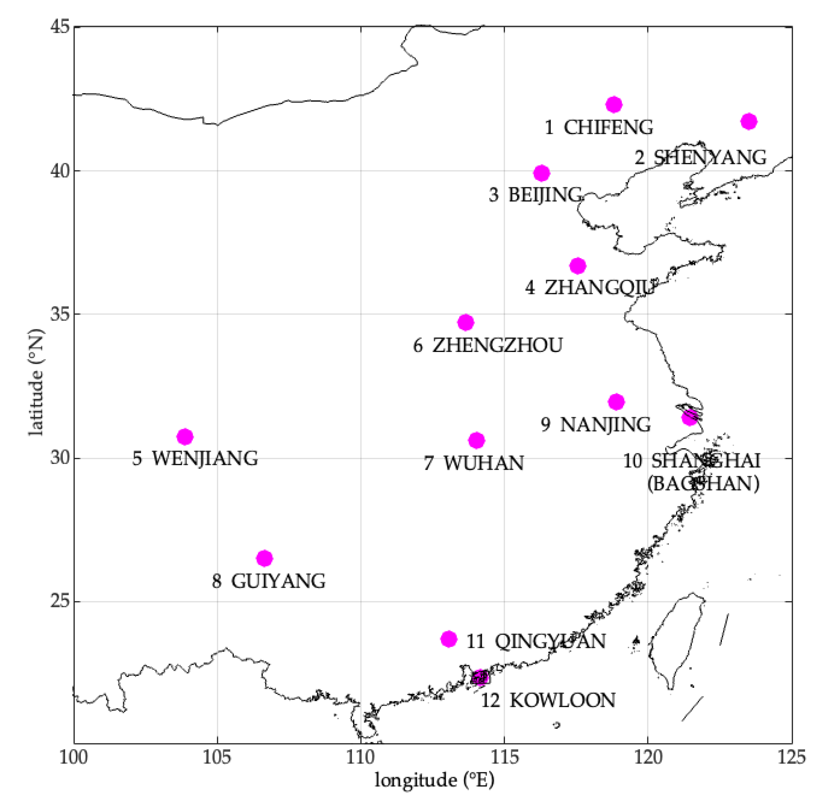
2.1. Data Description

Sounding data from 12 radiosonde stations located in the longitude range 100° E–125° E and latitude range 20° N–45° N in China throughout 12 years from 2008 to 2019 were downloaded from the Integrated Global Radiosonde Archive (IGRA) (at https://www.ncdc.noaa.gov/data-access/weather-balloon/integrated-global-radiosonde-archive (accessed on 23 February 2021)). The distribution of the 12 stations is shown in Figure 1. The main reason for the selection of these stations is that they had at least 10 continuous sounding layers containing the 10 standard pressure levels (1000, 925, 850, 700, 500, 400, 300, 250, 200) during the period of tests. The temporal resolution of the sounding data was 12 h (observed at 00:00 and 12:00 UTC). The vertical sounding profiles contain various meteorological measurements, including pressure, temperature, WV pressure, relative humidity, etc. at each sounding layer.

2.2. A New Parameter for the Vertical Distribution of Water Vapor

To obtain an accurate functional relationship between WV at two heights in the troposphere, a new WV parameter was introduced in this study (termed IRPWV), which reflects the variation of WV along the vertical direction. The derivation of its formula is as follows.
The ratio of PWV (noted as RPWV) at any two heights h i and h j ( h j > h i ) to TPWV in the troposphere is expressed as
RPWV i j = PWV h i h j TPWV
In general, PWV h i h j in Equation (6) is the numerical integral value of WVD from h i to h j ,
RPWV i j = ρ w i j Δ h i j TPWV
where ρ w i j is the mean WVD in the height range between h i and h j ; Δ h i j is thickness between h i and h j .
The above equation, by simple transformation, yields the following equation
IRPWV i , j = ρ w i j TPWV
where IRPWV i , j represents a per unit height (or thickness) of the ratio of PWV between h i and h j to TPWV, unit: 1/km.
When h i and h j are very close (i.e., a very thin layer), WVD i and WVD j are very close as well. Replacing the layer in Equation (8) with its corresponding mid-height h = h i + h j 2 , then Equation (8) can be expressed as
IRPWV h = ρ w h TPWV
Comparing the above equation with Equation (5), the similarity is the water vapor scale height H, which can be obtained from IRPWV h at the surface height, i.e., H = 1 / IRPWV s , but the difference is that Equation (5) takes the troposphere as a whole, while the above equation represents the variations of troposphere more finely. Meanwhile, the relation between WV can also be expressed in terms of IRPWV, as follows
ρ w l = ρ w k · IRPWV l IRPWV k
where ρ w l , ρ w k , IRPWV l and IRPWV k are the WVDs and IRPWVs at h l and h k , respectively.

2.3. Temporal Model

Considering the periodic characteristics of the IRPWV time-series over a site, the Fourier series below was used to fit IRPWV for the site in this study
f ( d o y ) = a 0 + i = 1 n ( a i cos ( i · d o y w ) + b i sin ( i · d o y w ) )
where i is the order of Fourier series; a 0 , a i and b i are the coefficients to be solved; doy is the day of year; w is the angular frequency.

3. Spatio–Temporal Characteristics of IRPWV and Modeling

The following procedures were carried out for the sounding data from each of the stations. First, according to Equations (2)–(4), the values of WVD at each of the sounding height layers, TPWV, and H were calculated; and then according to Equation (8), IRPWV at the mid-height of two adjacent heights h l = ( h i 1 + h i ) / 2 ( i is the index of the sounding height layer) was calculated. After this step was performed for all the sounding height layers across the 12 years and all the 12 stations on a doy-by-doy basis, the dataset containing d o y , h d o y , ρ w d o y , TPWV d o y , H d o y , h l d o y and IRPWV was obtained.

3.1. Temporal and Spatial Characteristics of IRPWV

The vertical distributions of IRPWV over the 10-year period from 2008 to 2017 at all the 12 stations are shown in Figure 2. We can see that the range of fluctuations of the IRPWV values decreases with an increase in altitude along the vertical direction at each station, and then it tends to be a steady value close to 0 at the highest altitudes. The vertical distribution ranges of IRPWV over all the stations are very similar. More specifically, the IRPWV fluctuation range varies with respect to the TPWV value, decreasing as the TPWV increases and vice versa.

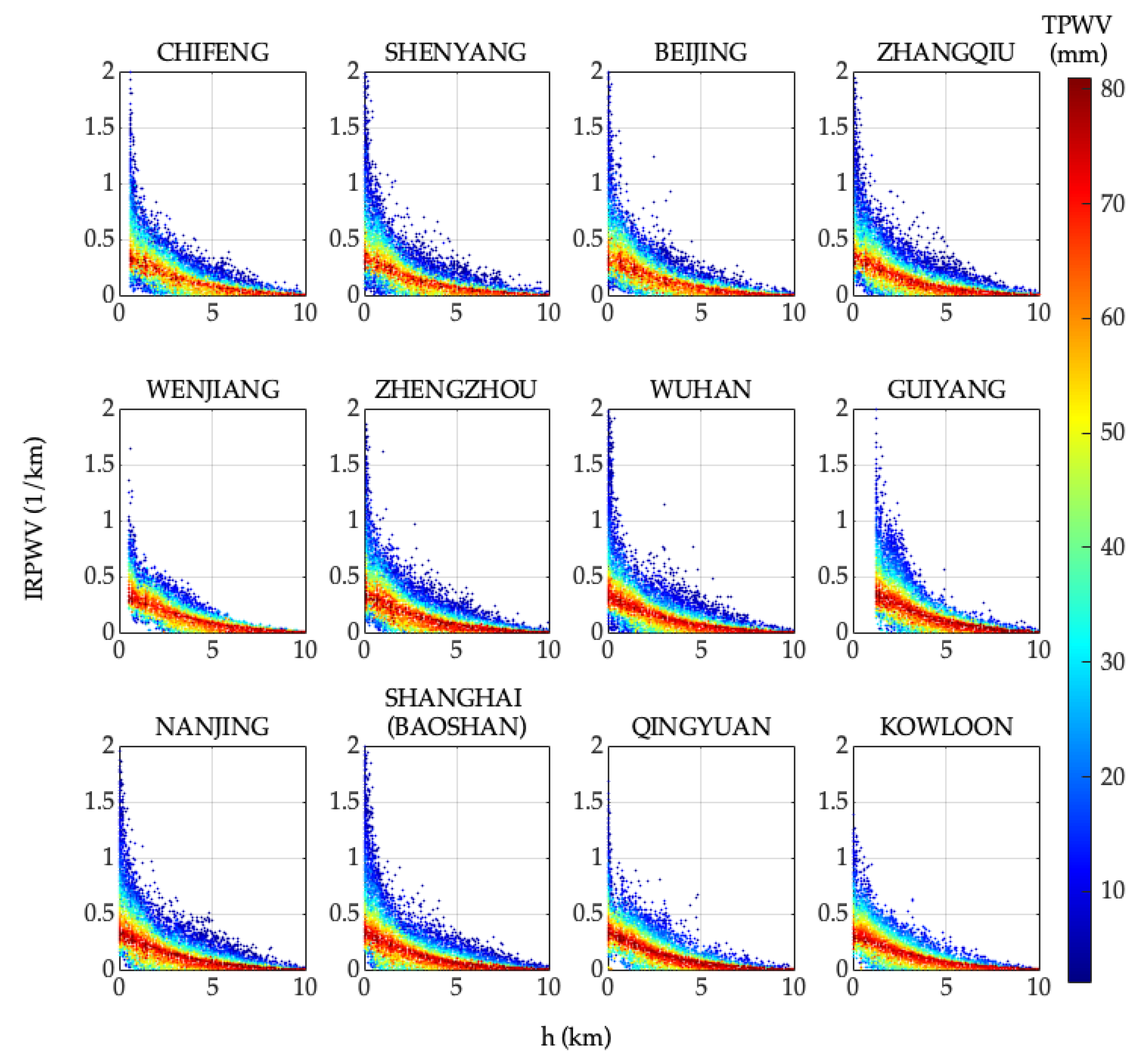
3.1.1. Statistical Characteristics of IRPWV

To analyze the temporal and spatial statistical characteristics of IRPWV, first, the aforementioned 10-year IRPWV time-series for each of the 12 stations were interpolated to 10 height layers, i.e., [ h s ,   1 ,   ,   10 ] (unit: km), where h s is the height of the station (note: h s is 1.223 km at GUIYANG station, therefore, its height layers are 9). Then, they were sorted monthly by their corresponding TPWV values and divided into 10 groups. Finally, the resultant newly sorted groups of IRPWV sample data will be used to calculate their monthly mean value and standard deviation (SD).
Figure 3a shows that, although the TPWV values in different months fall into different TPWV ranges, the mean value of IRPWV in each of the subfigures tends to be small with the increase in its corresponding TPWV in the same month, and eventually reaches a stable value. From January to July, the ranges of variation of the mean value are different, with the smallest in July and the largest in January. Mean IRPWV values at the same TPWV but in different TPWV ranges are different from each other and increase with the month. The results from July-to-December are the opposite of the January-to-July results. The trends shown in Figure 3b are consistent with the results of Figure 3a, the SD values decrease with the TPWV increases in the same time scale, i.e., for the maximum TPWV, its SD is the minimum. Each of the 12 stations shows the same characteristics described above, while the variation ranges of the monthly mean and SD values of the IRPWV are different from each other.
The above statistical results indicated that, within the same time scale, the IRPWV value correlates with the relative magnitude value of its corresponding TPWV compared to the other TPWV (those unlisted layers had the same characteristic), i.e., within a certain period, the IRPWV is dependent of the relative magnitude of TPWV, but not its corresponding TPWV value, which is denoted by Rel-TPWV hereafter in this paper, merely for convenience. In summary, while the Rel-TPWV is small, IRPWV has a larger range of fluctuations in its vertical distribution and vice versa.

3.1.2. Methodology for Determining Rel-TPWV

To obtain the vertical distribution of the IRPWV with respect to the TPWV at a certain time, it is necessary to establish a partitioning criterion for the TPWV, which is used to compare and determine its Rel-TPWV within the same time scale, and the following procedure is presented in this study.
Step 1, according to the periodic characteristics of the TPWV time series [42], a periodic function fitting the sample (i.e., measurements) of the 10-year TPWV d o y time series was obtained.
Step 2, the fitting function was applied to predict the TPWV value for each doy, which is denoted by TPWV f d o y , and the discrepancies (residuals) between the TPWV d o y and TPWV f d o y were calculated.
Step 3, the set of residuals for each doy over the duration of the 10 years was used to calculate the SD of TPWV for the doy, then according to the periodic characteristics of the time series of SD from doy 1 to 366, a fitting periodic model was obtained and applied to predict the SD for each doy, denoted by SD f d o y .
Step 4, both TPWV f d o y and SD f d o y on each doy were used to obtain five numerical boundaries for the doy, which are all based on the statistical theory that the probability of a value being within a ± 2 SD range is greater than or equal to 0.95 (percentile), as follows:
TPWV f d o y SD f d o y , TPWV f d o y 0.5 · SD f d o y , TPWV f d o y , TPWV f d o y + 0.5 · SD f d o y , and TPWV f d o y + SD f d o y .
Step 5, the above five numerical boundaries form six TPWV ranges (denoted by TPWV r , r = 1, 2, …, and 6) for each doy, i.e., the five numerical boundaries for all 366 doys form six TPWV r curves (see Figure 4), as follows:
TPWV 1 = [less than TPWV f d o y SD f d o y , TPWV f d o y SD f d o y ], TPWV 2 = [ TPWV f d o y SD f d o y , TPWV f d o y 0.5 · SD f d o y ], TPWV 3 = [ TPWV f d o y 0.5 · SD f d o y , TPWV f d o y ], TPWV 4 = [ TPWV f d o y , TPWV f d o y + 0.5 · SD f d o y ], TPWV 5 = [ TPWV f d o y + 0.5 · SD f d o y , TPWV f d o y + SD f d o y ], and TPWV 6 = [ TPWV f d o y + SD f d o y , greater than TPWV f d o y + SD f d o y ].
The six TPWV r were taken as the quantified and unified Rel-TPWV, e.g., if TPWV d o y values fall in the same TPWV r , they are considered to have the same Rel-TPWV value. Reflecting the results from the section above, that is, the vertical distribution of IRPWV is related to the Rel-TPWV of its corresponding TPWV in the same time session, e.g., if the Rel-TPWV of the vertical IRPWV distribution is larger than those of the others, the vertical IRPWV distribution is more stable and its fluctuation amplitude is also smaller than those of the others, and vice versa. The vertical distributions of IRPWV corresponding to the six TPWV r from 1 to 6 are considered as the following six vertical distributions of the WV: maximal-perturbation, sub-perturbation, normal-perturbation, normal-perturbation, least-perturbation, and least-perturbation, respectively.
According to the above partition criterion for TPWV, the 10-year sample data of IRPWV at 10 height layers were grouped by the TPWV r according to their corresponding TPWV d o y . The resultant new groups of IRPWV sample data will be used to study the characteristics of the temporal variations of IRPWV and the model for each group.

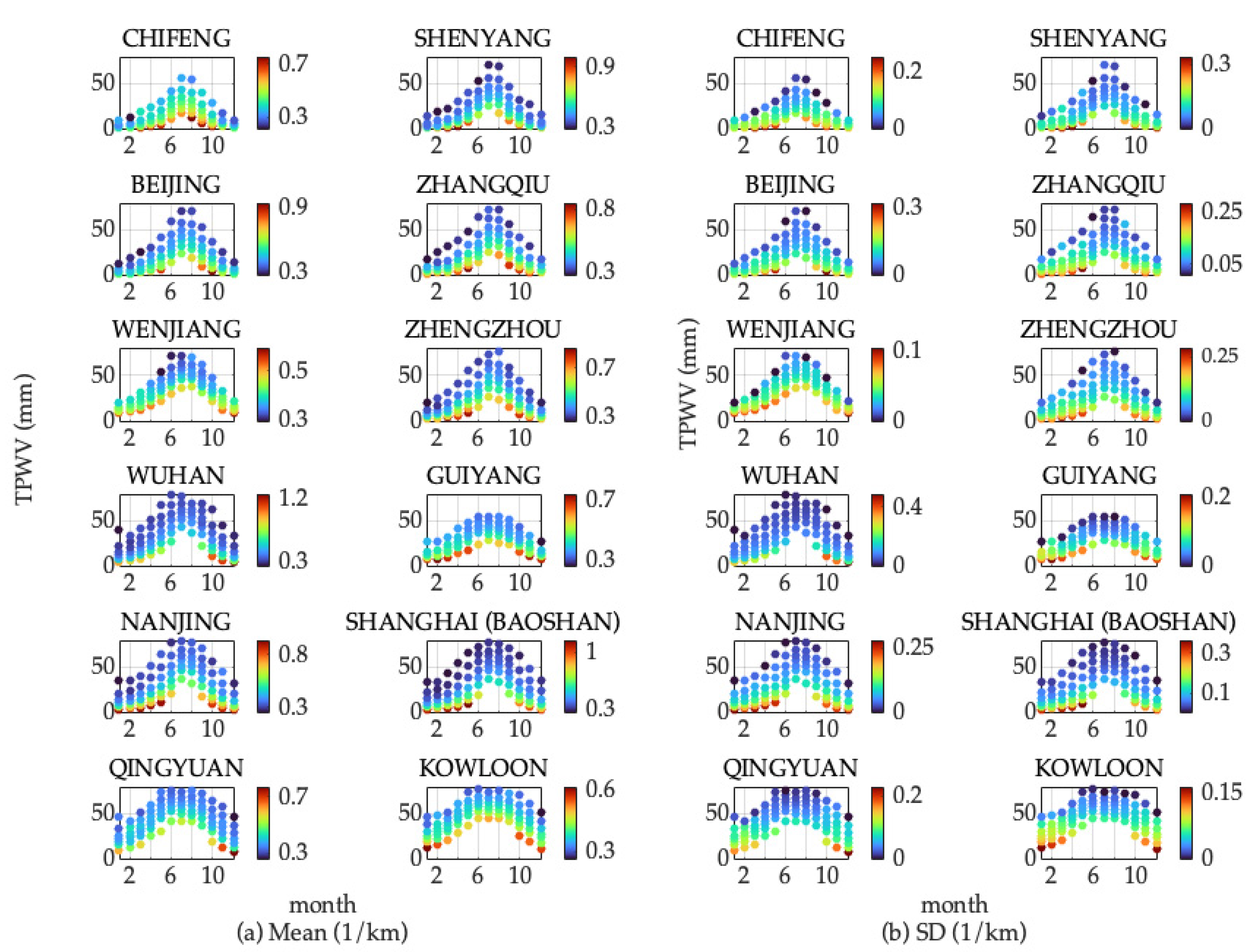
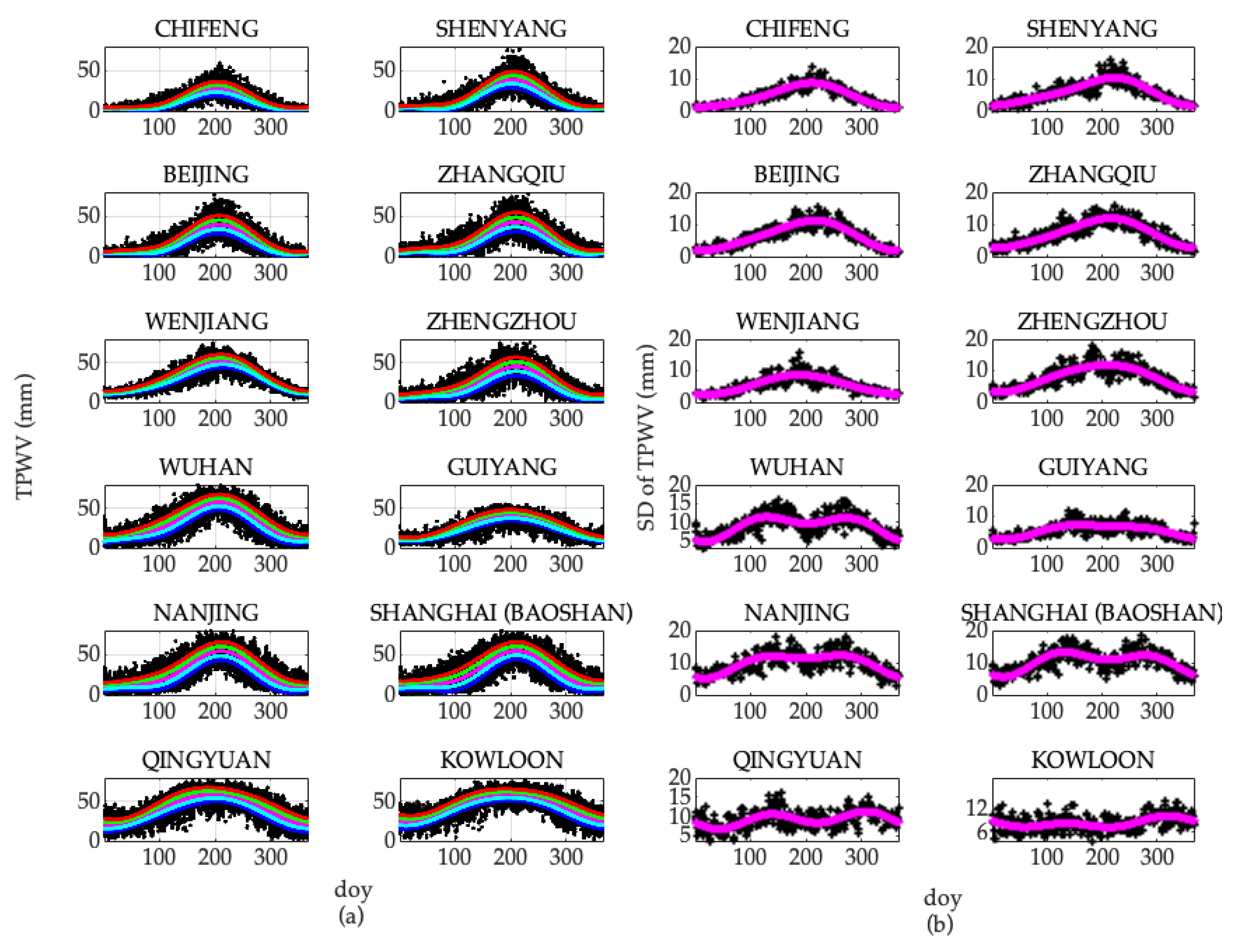
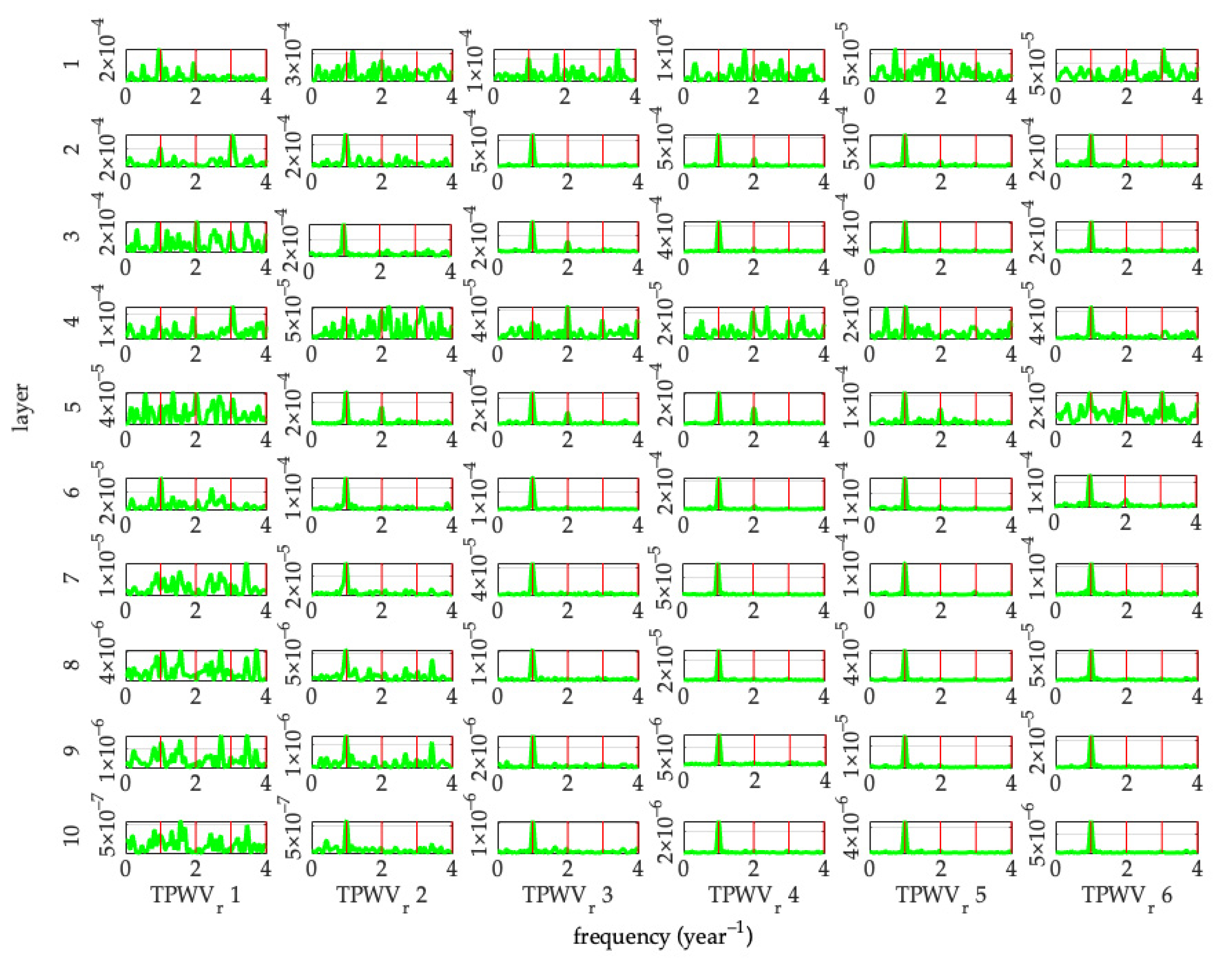
3.1.3. Temporal Characteristics of IRPWV

For the spectrum analysis of each group of the 10-year IRPWV time series at each of the 12 stations obtained in the previous section, the Fourier transform method was used, and results at the first layer (as an example) are shown in Figure 5 for the characteristics of the temporal variation of IRPWV of the stations.
As can be seen from Figure 5, the IRPWV time-series in each of the layers within six TPWV r generally present a clear periodic pattern, with significant annual and semi-annual periodic cycles. Different periodic characteristics of TPWV r are shown in different layers. In TPWV r 1, the annual and semi-annual cycles are significant at layers 1 and 6, and the semi-annual cycle is significant at layers 2 and 4, while at the other layers the annual, semi-annual, and 4-month cycles are equally significant to each other. In TPWV r 2–6, the annual cycle is significant and the semi-annual cycle is weak at layers 2, 3, 6–10, while at layer 5 the semi-annual cycle is equally significant with the annual cycle in TPWV r 6. In layers 1 and 4, the periods are different from each other.
With comprehensive consideration of the main annual and semi-annual periodic characteristics of the IRPWV time-series, the third order was adopted as its fitting function in Equation (10). It should be noted that the 4-month periodic characteristic may be insignificant or not even present in an IRPWV time-series. In this case, the coefficient of the 4-month term in Equation (10) will be very small or even close to 0. Consequently, the trigonometric function contains only annual and semi-annual periodic terms. Results from the other stations were also investigated, and the same temporal variability pattern was observed, although the IRPWV fluctuations were different for different groups and different stations. The spatio-temporal modeling for each of the groups of the 10-year IRPWV data will be carried out in the next section.

3.2. Construction of Spatio-Temporal IRPWV Model

According to the classification of WV vertical distribution in Section 3.2, the vertical distribution of IRPWV in the TPWV r is considered as a type of WV vertical distribution, and the true vertical distribution of IRPWV can be generalized as
IRPWV = IRPWV r + perturbation r
where IRPWV r and perturbation r are the IRPWV and its perturbation term in the corresponding TPWV r , respectively; r is from 1 to 6.
Based on the annual and semi-annual periodic characteristics of the IRPWV time-series in each layer within each TPWV r , Equation (10) (taking the third-order) was adopted as the fitting model for each of the groups of the 10-year IRPWV sample data
IRPWV h , r = a 0 , h , r + a 1 , h , r cos ( d o y w ) + b 1 , h , r sin ( d o y w ) + a 2 , h , r cos ( d o y 2 w ) + b 2 , h , r sin ( d o y 2 w ) + a 3 , h , r cos ( d o y 3 w ) + b 3 , h , r sin ( d o y 3 w )
where a 0 , h , r , a 1 , h , r , b 1 , h , r , a 2 , h , r , b 2 , h , r , a 3 , h , r and b 3 , h , r are the coefficients of the periodic terms; the subscripts h and r are the indexes of the height layer and TPWV r , respectively; w = 2 π / 365.25 . The coefficients for each group of the IRPWV sample data for the KOWLOON station (as an example) are partially selected and shown in Table 1.

4. Evaluation of IRPWV Model

To validate the aforementioned constructed IRPWV models, the WVD values for each doy in 2018 and 2019 predicted by the IRPWV model and the commonly used exponential model containing H (named ρ w m and ρ w H , respectively) were compared against the reference values in the same two years using the procedure introduced in Section 3.1. Since there are no global H models available at present, according to the periodic characteristics of H [36,37], instead, the coefficients of the periodic model of H over each station were obtained from the H d o y time series in the 10 years from 2008 to 2017 by Equation (10) (the second-order was adopted). The validation procedure is as follows.
(1) Validation of model-predicted ρ w m and ρ w H in two cases below.
According to the Rel-TPWV of TPWV relative to TPWV r on the same doy at a station site, the periodic function coefficients in each height layer within the corresponding TPWV r were selected, and the doy in 2018 and 2019 were used as the input of Equation (12) to calculate the IRPWV h , r value for the doy. The H on the same doy in 2018 and 2019 resulting from the H model was obtained using the coefficients of the periodic H model of the same station, noted as H m .
Case 1: ρ w m and ρ w H resulting from two models and TPWV.
For the same station site, ρ w H at the surface and ρ w m in each height layer on the same doy were calculated using the following two equations
ρ w H s = TPWV ρ w H
ρ w m h r = TPWV · IRPWV h , r
Then, for the i th sounding height layer, ρ w H i and ρ w m i at height h d o y i were calculated by Equation (1) and interpolation between ( h r 1 , ρ w m h r 1 ) and ( h r 2 , ρ w m h r 2 ) (where h r 1 < h d o y i < h r 2 ) , respectively.
Case 2: ρ w m and ρ w H resulting from two models and WVD at a specific altitude.
For the same station, ρ w m j and ρ w H j at height h j were calculated from the WVD ( ρ w i ) at the height h i ( i and j are the indexes of the sounding layer from 1 to the last, respectively, and i j ) using the following equations
ρ w m j = ρ w i · IRPWV j , r IRPWV i , r
ρ w H j = ρ w i exp ( ( h j h i ) / H m )
where IRPWV i , r and IRPWV j , r were obtained by interpolating ( h r 1 , ρ w m h r 1 ) and ( h r 2 , ρ w m h r 2 ), ( h r 3 , ρ w m h r 3 ) and ( h r 4 , ρ w m h r 4 ), respectively, where h r 1 < h d o y i < h r 2 , h r 3 < h d o y i < h r 4 , for an example.
(2) Using the above procedure to obtain ρ w m and ρ w H for all doys in 2018 and 2019 for each of the 12 stations, then the statistics including annual bias and root mean square error (RMSE) of the differences between the model-predicted results and reference values were calculated for the models’ performance indicators. The formulas of the bias and RMSE are
bias = 1 n i = 1 n ( V a l u e m i V a l u e r i )
RMSE = 1 n i = 1 n ( V a l u e m i V a l u e r i ) 2
where i is the index of the sample data; the subscriptions m and r denote model and reference, respectively; n is the number of the samples contained in the statistics.
For each of the 12 stations, ρ w m and ρ w H for all doys in 2018 and 2019 were obtained from the two models and TPWV and ρ w , respectively. The results were then divided into 10 groups of 1 km interval starting from the station altitude along the vertical direction. Their corresponding reference values obtained from the sounding data in the same 10 height ranges were used to evaluate the performance of the two models in each height interval. The bias and RMSE results are shown in the next two sections.

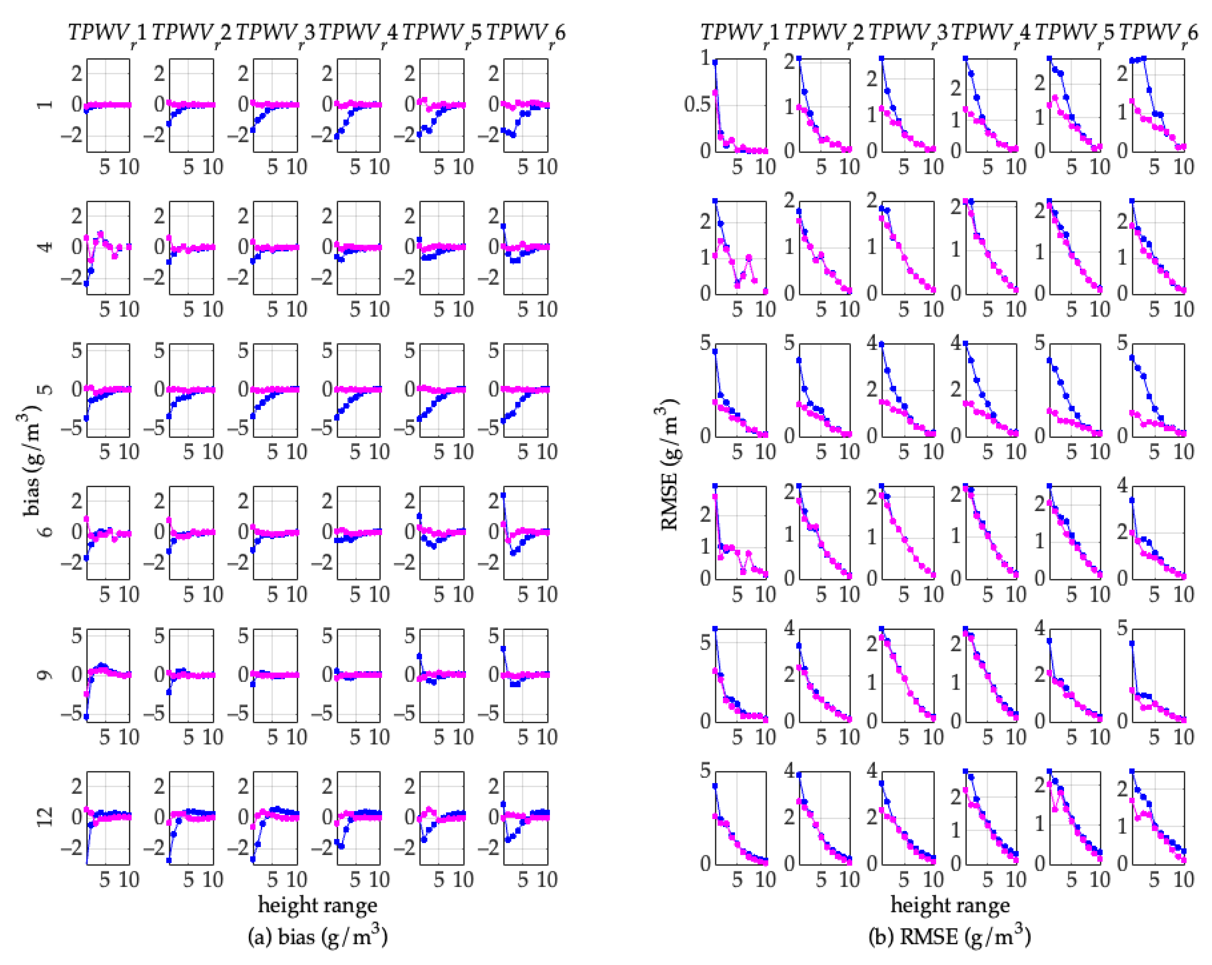
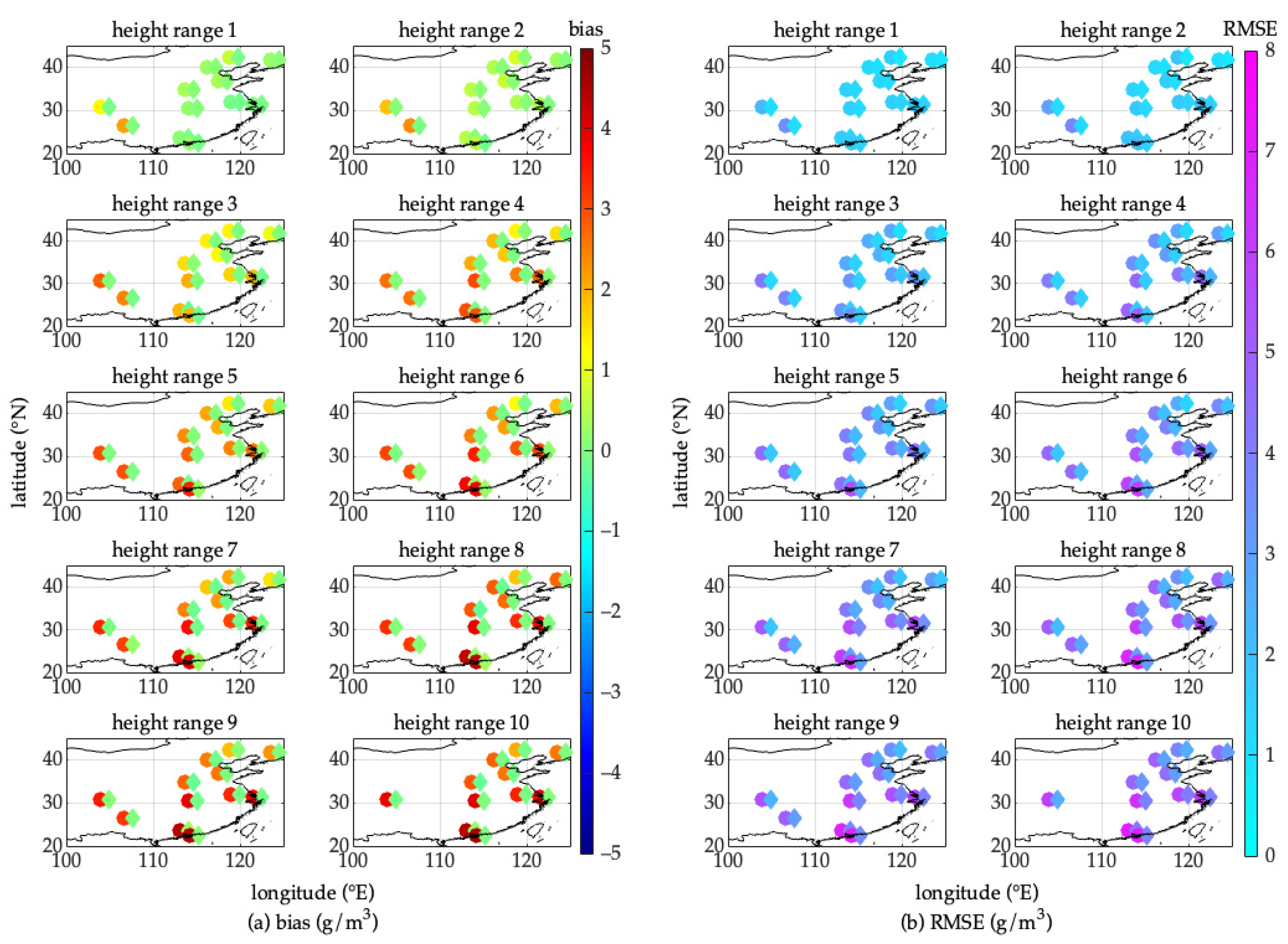
4.1. Accuracy of WVD Resulting from Models and TPWV

In Figure 6, considering both the bias and RMSE, it can be seen that, at stations 1, 5, and 12, the annual biases of ρ w m are close to 0 in all 10 height ranges within all TPWV r , and that of ρ w H all increase from a small negative value to 0 with the increase in height within all six TPWV r . In addition, the annual RMSEs of ρ w H at these three stations are at least about two times that of ρ w m . The bias and RMSE values of the exponential model at station 5 in the height range from 1 to 5 are about from –4 to –2.5 g/m3, and from 1 to 4.5 g/m3, respectively. This performance of the exponential model is poor. At stations 4, 6, and 9 and in the same low height ranges, e.g., from 1 to 5, their absolute bias and RMSE values vary with the variation of TPWV r from 1 to 6, e.g., the two values in TPWV r 3 and 4 are less than that in the other TPWV r , which reflects that the exponential model is only suitable to the normal water vapor state. Note that since WV content in a low-height layer is much larger than that in a high layer, this section mainly focuses on the results in low-height layers. Based on both the bias and RMSE of ρ w m and ρ w H resulting from the two models and TPWV d o y , the new model is superior to the commonly used exponential model in all height ranges within all six TPWV r at all stations (the same results were also found from the other six unlisted stations).
Due to the difficulty of finding the difference between the RMSEs of ρ w m and ρ w H in greater height ranges in Figure 6b, we counted the improvement ratios of the annual RMSE of ρ w m relative to that of ρ w H in the 10 height ranges within all TPWV r at the 12 stations, and the results are shown in Figure 7. It can be seen that the proportions of the number of the height ranges that had reduced the annual RMSE of ρ w m to all 10 height ranges within all six TPWV r (i.e., a total of 60 height ranges) are from 75% to 80% at the CHIFENG, BEIJING, ZHENGZHOU, and ZHANGQIU stations; and the results at the other stations were all over 90%.

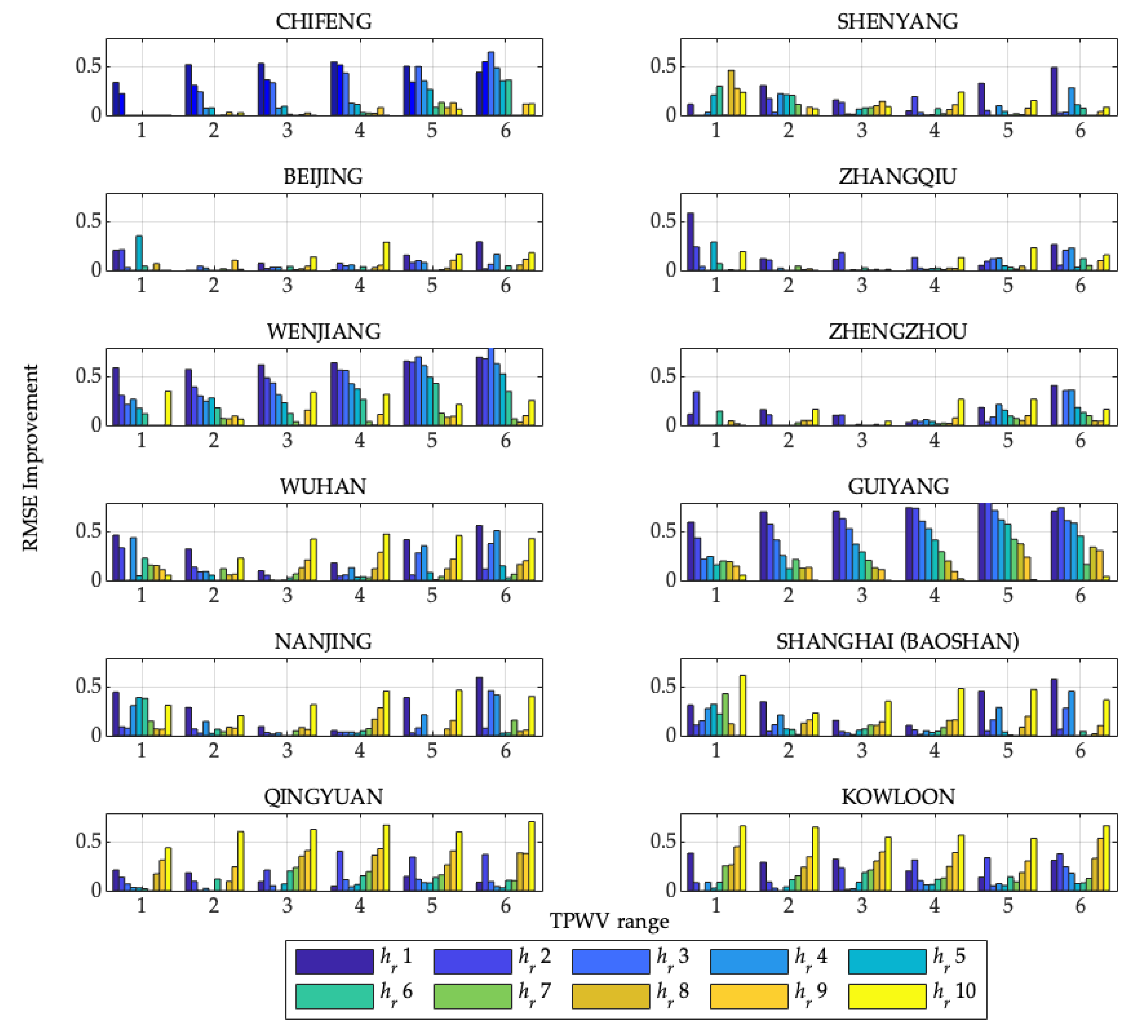
4.2. Accuracy of WVD Resulting from Models and WVD at a Specific Altitude

Figure 8a shows that the annual biases of ρ w H at all the 12 stations increase gradually with the increase in the height of ρ w , and in the height range 2 or above, they are all above 0, which indicates that the exponential model only performs well within the height range 1, and all the positive bias values mean systematic overestimation of the model. In contrast, the biases of ρ w m in the 10 height ranges all float around the 0 value. In Figure 8b, the annual RMSEs of the two models at the 12 stations all show a tendency of larger RMSE in greater height ranges, i.e., the RMSE increases with the increase in the height of ρ w , with different amounts of increase. Therein, the minimum increment in the RMSE of ρ w H is 1.5 g/m3 (from 3.5 to 5.0 g/m3), and is at GUIYANG, where the RMSE of ρ w m is from 1.1 to 3.1 g/m3; the maximum increment is 5.4 g/m3 (from 1.7 to 7.1 g/m3) and is at KOWLOON, where the RMSE of ρ w m is from 1.4 to 3.9 g/m3. Noticeably, the RMSE of ρ w m is less than that of ρ w H in all 10 height ranges. Compared with the ρ w H result, the RMSEs of ρ w m at all stations in each of the 10 height ranges reduce at least 11%, 20%, 43%, 48%, 40%, 38%, 32%, 35%, 32% and 28%, see Figure 8c.
From the above results, it can be concluded that WVD at a lower height has resulted from the model and WVD at a greater height, while the small variation in the latter WVD (the variation in WVD at a greater height is small relative to WVD at the lower heights, but is large relative to WVD at the greater heights) has a great impact on the former. In addition, the poor result of the exponential model is also caused by the fact that the model is based on the exponential decline trend along with the vertical range from the surface WVD to the tropopause. Therefore, the new model is superior to the exponential model because it reflects the relationship between WVDs at different heights. In addition, when the new model is applied, the WVD at a lower height should be selected as far as possible to calculate the WVD at a greater height through the model.

5. Conclusions

Water vapor in the troposphere varies with time and space. Its vertical distribution is correlated with the state of the atmosphere, such as the meteorological factors of, e.g., the column water vapor, temperature, and water vapor pressure. For better modeling of the variations in the vertical distribution of water vapor under different amounts of the total precipitable water vapor (TPWV), a new water vapor parameter, IRPWV (the ratio of water vapor density to the TPWV), was designed.
From the analyses of the vertical distribution of IRPWV time-series obtained from the 10-year sounding data over 12 radiosonde stations in China, it was found that the vertical distribution of the IRPWV time-series not only strongly correlated with the relative magnitude of its corresponding TPWV at the same time over the same site, but also presents a periodic variation pattern in the temporal domain. To quantify the relative magnitude of TPWV and unify the criteria for the relative magnitude, six TPWV ranges time-series (from 1 to 6) were developed by the periodic function of TPWV and its standard deviation. They were then used to classify the vertical distributions of IRPWV into six vertical distributions of water vapor by their corresponding TPWVs. For the periodic variations in each of the six classified IRPWVs, a temporal IRPWV model is developed with six sets of coefficients for fitting the six classified vertical distributions of IRPWV. The new fitting model was evaluated by comparing its prediction against the radiosonde data as references in 2018 and 2019 (out-of-sample data), and its performance was also assessed against the commonly used exponential model. Results showed that the new IRPWV model significantly outperformed the exponential model in the following aspects: First, the proportions of the number of the height ranges that had reduced annual root mean square error (RMSE) of water vapor density (WVD) obtained from the new model and TPWV in all height ranges were from 75% to 80% at the CHIFENG, BEIJING, ZHENGZHOU, and ZHANGQIU stations; the results at other stations were all above 90%. Secondly, considering all six TPWV ranges and all stations as a whole, the annual RMSEs of WVDs obtained from the new model and WVDs in the height range from 1 to 10 were reduced by at least 11%, 20%, 43%, 48%, 40%, 38%, 32%, 35%, 32%, and 28%, respectively. All results suggest that, for different water vapor states, the new IRPWV fitting model performs well in reflecting not only the temporal relationship between the WVDs and the TPWV but also the vertical distribution of WVDs at different altitudes well.

Supplementary Materials

The following supporting information can be downloaded at: https://www.mdpi.com/article/10.3390/atmos13122039/s1. Figures S1–S9: Monthly IRPWV mean (a) and SD (b) values (unit: 1/km) of each of the TPWV groups which are sorted by their corresponding TPWV in the layer 2–10 at each of the 12 stations.; Figures S10–S20: Power-period of 10-year IRPWV time series of the 10 layers within six TPWV r at CHIFENG, SHENYANG, BEIJING, ZHENGZHOU, WENJIANG, ZHENGZHOU, WUHAN, GUIYANG, NANJING, SHANGHAI(BAOSHAN), and QINGYUAN stations, respectively. Table S1: Coefficients of the IRPWV model for all the layers within the six TPWV r at the 12 stations.

Author Contributions

M.W., K.Z., S.W., Z.S., P.S. and L.L. contributed to the study’s conception and design. Material preparation, data collection, and analysis were performed by M.W. The first draft of the manuscript was written by M.W. and K.Z.; S.W., Z.S., P.S. and L.L. commented on previous versions of the manuscript. All authors have read and agreed to the published version of the manuscript.

Funding

This research was funded by the Natural Science Foundation of China (Grant No. 42274021, 41874040, 41730109), the Construction Program of Space-Air-Ground-Well Cooperative Awareness Spatial Information Project (Grant No. B20046), the Independent Innovation Project of “Double-First Class” Construction (Grant No. 2022ZZCX06), and 2022 Jiangsu Provincial Science and Technology Initiative—Special Fund for International Science and Technology Cooperation (Grant No. BZ2022018).

Data Availability Statement

The radiosonde data can be downloaded from: https://www.ncdc.noaa.gov/data-acces s/weather-balloon/integrated-global-radiosonde-archive (accessed on 23 February 2021).

Acknowledgments

We acknowledge the National Oceanic and Atmospheric Administration (NOAA) for the provision of the Integrated Global Radiosonde Archive (IGRA) datasets.

Conflicts of Interest

The authors declare no conflict of interest.

Appendix A

Table A1. Coefficients of the IRPWV model for all the layers within the six TPWV r at KOWLOON station.
TPWV RangeCoefficientHeight Layer
12345678910
1 a 0 0.5180.3360.1920.1150.0640.0360.0210.0140.0080.005
a 1 0.0480.011−0.0050.001−0.008−0.008−0.0020.0000.0000.000
b 1 0.003−0.0170.0010.008−0.0010.0020.0000.0020.0020.001
a 2 0.022−0.0040.015−0.004−0.008−0.0030.0000.0000.0000.000
b 2 0.0150.0000.003−0.002−0.006−0.0020.000−0.001−0.0010.000
a 3 −0.013−0.0160.0150.001−0.0020.0000.0030.0020.0010.000
b 3 0.0190.014−0.003−0.012−0.006−0.0010.0010.0000.0000.000
2 a 0 0.4340.3240.2220.1290.0680.0370.0200.0120.0070.004
a 1 0.0170.0240.022−0.002−0.022−0.016−0.008−0.003−0.002−0.001
b 1 −0.011−0.0020.0110.005−0.004−0.003−0.003−0.0010.0000.000
a 2 0.0160.0060.008−0.009−0.015−0.0010.0010.0010.0000.000
b 2 0.0140.0080.005−0.002−0.008−0.004−0.002−0.0010.0000.000
a 3 −0.001−0.0030.006−0.005−0.0030.0030.0010.0020.0010.000
b 3 0.0140.006−0.002−0.005−0.0020.0000.000−0.0010.0000.000
3 a 0 0.4100.3240.2220.1310.0720.0390.0220.0120.0070.004
a 1 0.0100.0340.025−0.005−0.021−0.018−0.009−0.005−0.003−0.002
b 1 −0.0090.0070.0110.003−0.005−0.007−0.004−0.0020.0000.000
a 2 0.0090.0050.007−0.009−0.010−0.0010.0000.0010.0010.001
b 2 0.0010.0040.012−0.002−0.007−0.004−0.002−0.0010.0000.000
a 3 0.0020.0010.004−0.004−0.0040.0010.0000.0000.0000.000
b 3 0.003−0.0010.002−0.005−0.0010.0020.001−0.001−0.0010.000
4 a 0 0.3840.3090.2210.1380.0760.0430.0250.0150.0080.004
a 1 0.0050.0300.0310.004−0.019−0.021−0.013−0.008−0.004−0.003
b 1 −0.0030.0140.0080.001−0.007−0.007−0.004−0.002−0.0010.000
a 2 0.0050.0030.004−0.004−0.008−0.0020.0010.0010.0010.001
b 2 0.0050.0120.006−0.005−0.011−0.004−0.002−0.0010.0000.000
a 3 0.0030.0000.001−0.001−0.0030.0010.0010.0000.0010.000
b 3 0.0060.0060.000−0.005−0.0050.0000.0010.0000.0000.000
5 a 0 0.3640.2980.2180.1400.0850.0500.0290.0170.0090.005
a 1 0.0030.0280.0280.006−0.012−0.018−0.013−0.009−0.005−0.003
b 1 0.0010.0170.0110.001−0.009−0.009−0.006−0.003−0.001−0.001
a 2 0.0010.0000.004−0.002−0.004−0.0020.0010.0010.0010.001
b 2 0.0060.0110.005−0.001−0.010−0.005−0.0010.0000.0000.000
a 3 0.000−0.004−0.0020.0010.0000.0010.0020.0010.0000.000
b 3 0.0040.0040.000−0.003−0.0050.0010.0010.0010.0000.000
6 a 0 0.3380.2830.2110.1430.0930.0570.0350.0200.0110.006
a 1 −0.0050.0220.0220.010−0.002−0.013−0.013−0.010−0.007−0.004
b 1 0.0040.0160.0090.000−0.005−0.009−0.007−0.004−0.002−0.001
a 2 −0.007−0.0030.0020.0030.002−0.001−0.0010.0000.0000.000
b 2 0.0040.0100.006−0.001−0.006−0.007−0.003−0.0010.0000.000
a 3 −0.008−0.010−0.0040.0020.0060.0040.0020.0010.0010.000
b 3 0.0040.0020.000−0.001−0.003−0.0010.0000.0000.0000.000

References

  1. Chahine, M.T. The Hydrological Cycle and Its Influence on Climate. Nature 1992, 359, 373–380. [Google Scholar] [CrossRef]
  2. Viswanadham, Y. The Relationship between Total Precipitable Water and Surface Dew Point. J. Appl. Meteorol. 1981, 20, 3–8. [Google Scholar] [CrossRef]
  3. Rocken, C.; van Hove, T.; Ware, R. Near Real-Time GPS Sensing of Atmospheric Water Vapor. Geophys. Res. Lett. 1997, 24, 3221–3224. [Google Scholar] [CrossRef] [Green Version]
  4. Bevis, M.; Businger, S.; Herring, T.A.; Rocken, C.; Anthes, R.A.; Ware, R.H. GPS Meteorology: Remote Sensing of Atmospheric Water Vapor Using the Global Positioning System. J. Geophys. Res. 1992, 97, 15787. [Google Scholar] [CrossRef]
  5. Liu, Z.; Wong, M.S.; Nichol, J.; Chan, P.W. A Multi-Sensor Study of Water Vapour from Radiosonde, MODIS and AERONET: A Case Study of Hong Kong. Int. J. Climatol. 2013, 33, 109–120. [Google Scholar] [CrossRef] [Green Version]
  6. Zhao, T.; Dai, A.; Wang, J. Trends in Tropospheric Humidity from 1970 to 2008 over China from a Homogenized Radiosonde Dataset. J. Clim. 2012, 25, 4549–4567. [Google Scholar] [CrossRef] [Green Version]
  7. Jacob, D. The Role of Water Vapour in the Atmosphere. A Short Overview from a Climate Modeller’s Point of View. Phys. Chem. Earth Part A Solid Earth Geod. 2001, 26, 523–527. [Google Scholar] [CrossRef]
  8. Huang, L.; Mo, Z.; Xie, S.; Liu, L.; Chen, J.; Kang, C.; Wang, S. Spatiotemporal Characteristics of GNSS-Derived Precipitable Water Vapor during Heavy Rainfall Events in Guilin, China. Satell. Navig. 2021, 2, 13. [Google Scholar] [CrossRef]
  9. Huang, L.; Mo, Z.; Liu, L.; Zeng, Z.; Chen, J.; Xiong, S.; He, H. Evaluation of Hourly PWV Products Derived From ERA5 and MERRA-2 Over the Tibetan Plateau Using Ground-Based GNSS Observations by Two Enhanced Models. Earth Space Sci. 2021, 8, e2020EA001516. [Google Scholar] [CrossRef]
  10. Keil, C.; Röpnack, A.; Craig, G.C.; Schumann, U. Sensitivity of Quantitative Precipitation Forecast to Height Dependent Changes in Humidity. Geophys. Res. Lett. 2008, 35, 1–5. [Google Scholar] [CrossRef]
  11. Schiro, K.A.; Neelin, J.D.; Adams, D.K.; Lintner, B.R. Deep Convection and Column Water Vapor over Tropical Land versus Tropical Ocean: A Comparison between the Amazon and the Tropical Western Pacific. J. Atmos. Sci 2016, 73, 4043–4063. [Google Scholar] [CrossRef]
  12. Weckwerth, T.M.; Parsons, D.B. A Review of Convection Initiation and Motivation for IHOP_2002. Mon. Weather Rev. 2006, 134, 5–22. [Google Scholar] [CrossRef]
  13. Sherwood, S.C.; Roca, R.; Weckwerth, T.M.; Andronova, N.G. Tropospheric Water Vapor, Convection, and Climate. Rev. Geophys. 2010, 48, 1–29. [Google Scholar] [CrossRef] [Green Version]
  14. Rose, B.E.J.; Rencurrel, M.C. The Vertical Structure of Tropospheric Water Vapor: Comparing Radiative and Ocean-Driven Climate Changes. J. Clim. 2016, 29, 4251–4268. [Google Scholar] [CrossRef]
  15. Renju, R.; Raju, C.S.; Mathew, N.; Antony, T.; Moorthy, K.K. Microwave Radiometer Observations of Interannual Water Vapor Variability and Vertical Structure over a Tropical Station. J. Geophys. Res. 2015, 120, 4585–4599. [Google Scholar] [CrossRef]
  16. Lintner, B.R.; Holloway, C.E.; Neelin, J.D. Column Water Vapor Statistics and Their Relationship to Deep Convection, Vertical and Horizontal Circulation, and Moisture Structure at Nauru. J. Clim. 2011, 24, 5454–5466. [Google Scholar] [CrossRef]
  17. Holloway, C.E.; Neelin, D.J. Moisture Vertical Structure, Column Water Vapor, and Tropical Deep Convection. J. Atmos. Sci. 2009, 66, 1665–1683. [Google Scholar] [CrossRef] [Green Version]
  18. Schneider, T.; O’Gorman, P.A.; Levine, X.J. Water Vapor and the Dynamics of Climate Changes. Rev. Geophys. 2010, 48, 1–22. [Google Scholar] [CrossRef] [Green Version]
  19. Trenberth, K.E.; Fasullo, J.T.; Mackaro, J. Atmospheric Moisture Transports from Ocean to Land and Global Energy Flows in Reanalyses. J. Clim. 2011, 24, 4907–4924. [Google Scholar] [CrossRef]
  20. Huang, L.; Wang, X.; Xiong, S.; Li, J.; Liu, L.; Mo, Z.; Fu, B.; He, H. High-Precision GNSS PWV Retrieval Using Dense GNSS Sites and in-Situ Meteorological Observations for the Evaluation of MERRA-2 and ERA5 Reanalysis Products over China. Atmos. Res. 2022, 276, 106247. [Google Scholar] [CrossRef]
  21. Huang, L.; Mo, Z.; Liu, L.; Xie, S. An Empirical Model for the Vertical Correction of Precipitable Water Vapor Considering the Time-Varying Lapse Rate for Mainland China. Cehui Xuebao/Acta Geod. Cartogr. Sin. 2021, 50, 1320. [Google Scholar] [CrossRef]
  22. Zhang, H.; Yuan, Y.; Li, W.; Zhang, B. A Real-Time Precipitable Water Vapor Monitoring System Using the National GNSS Network of China: Method and Preliminary Results. IEEE J. Sel. Top. Appl Earth Obs. Remote Sens. 2019, 12, 1587–1598. [Google Scholar] [CrossRef]
  23. Reitan, C.H. Surface Dew Point and Water Vapor Aloft. J. Appl. Meteorol. 1963, 2, 776–779. [Google Scholar] [CrossRef]
  24. Smith, W.L. Note on the Relationship Between Total Precipitable Water and Surface Dew Point. J. Appl. Meteorol. 1966, 5, 726–727. [Google Scholar] [CrossRef]
  25. Raymond, W.H. Estimating Moisture Profiles Using a Modified Power Law. J. Appl. Meteorol. 2000, 39, 1059–1070. [Google Scholar] [CrossRef]
  26. Smith, W.L.; Feltz, W.F.; Knuteson, R.O.; Revercomb, H.E.; Woolf, H.M.; Howell, H.B. The Retrieval of Planetary Boundary Layer Structure Using Ground-Based Infrared Spectral Radiance Measurements. J. Atmos. Ocean. Technol. 1999, 16, 323–333. [Google Scholar] [CrossRef]
  27. Kalnay, E. Atmospheric Modeling, Data Assimilation and Predictability; Cambridge University Press: Cambridge, UK, 2002. [Google Scholar]
  28. Chaboureau, J.P. Relationship between Sea Surface Temperature, Vertical Dynamics, and the Vertical Distribution of Atmospheric Water Vapor Inferred from TOVS Observations. J. Geophys. Res. Atmos. 1998, 103, 8743–8752. [Google Scholar] [CrossRef] [Green Version]
  29. Reber, E.E.; Swope, J.R. On the Correlation of the Total Precipitable Water in a Vertical Column and Absolute Humidity at the Surface. J. Appl. Meteorol. 1972, 11, 1322–1325. [Google Scholar] [CrossRef]
  30. Tomasi, C. Determination of the Total Precipitable Water by Varying the Intercept in Reitan’s Relationship. J. Appl. Meteorol. 1981, 20, 1058–1069. [Google Scholar] [CrossRef]
  31. Byers, H.R. Significance of Different Vertical Distributions of Water Vapor in Arid and Humid Regions. J. Meteorol. Soc. Japan. Ser. II 1957, 35A, 330–335. [Google Scholar] [CrossRef]
  32. Tomasi, C. Precipitable Water Vapor in Atmospheres Characterized by Temperature Inversions. J. Appl. Meteorol. 1977, 16, 237–243. [Google Scholar] [CrossRef]
  33. Weaver, C.P.; Ramanathan, V. Deductions from a Simple Climate Model: Factors Governing Surface Temperature and Atmospheric Thermal Structure. J. Geophys Res. 1995, 100, 11585. [Google Scholar] [CrossRef]
  34. John, T.; Garg, S.C.; Maini, H.K.; Chaunal, D.S.; Yadav, V.S. Design of a Simple Low Cost Tethersonde Data Acquisition System for Meteorological Measurements. Rev. Sci. Instrum. 2005, 76, 84501. [Google Scholar] [CrossRef]
  35. Kennett, E.J.; Toumi, R. Temperature Dependence of Atmospheric Moisture Lifetime. Geophys. Res. Lett. 2005, 32, 1–4. [Google Scholar] [CrossRef]
  36. Otarola, A.C.; Querel, R.; Kerber, F. Precipitable Water Vapor: Considerations on the Water Vapor Scale Height, Dry Bias of the Radiosonde Humidity Sensors, and Spatial and Temporal Variability of the Humidity Field. 2011. Available online: https://arxiv.org/abs/1103.3025 (accessed on 12 December 2021).
  37. Zhang, B.; Yao, Y.; Xu, C. Global Empirical Model for Estimating Water Vapor Scale Height. Cehui Xuebao/Acta Geod. Cartogr. Sin. 2015, 44, 1085–1091. [Google Scholar] [CrossRef]
  38. Romps, D.M. An Analytical Model for Tropical Relative Humidity. J. Clim. 2014, 27, 7432–7449. [Google Scholar] [CrossRef]
  39. Fischer, L.; Craig, G.C.; Kiemle, C. Horizontal Structure Function and Vertical Correlation Analysis of Mesoscale Water Vapor Variability Observed by Airborne Lidar. J. Geophys. Res. Atmos. 2013, 118, 7579–7590. [Google Scholar] [CrossRef] [Green Version]
  40. Iassamen, A.; Sauvageot, H.; Jeannin, N.; Ameur, S. Distribution of Tropospheric Water Vapor in Clear and Cloudy Conditions from Microwave Radiometric Profiling. J. Appl. Meteorol. Clim. 2009, 48, 600–615. [Google Scholar] [CrossRef]
  41. Lintner, B.R.; Adams, D.K.; Schiro, K.A.; Stansfield, A.M.; Amorim Rocha, A.A.; Neelin, J.D. Relationships among Climatological Vertical Moisture Structure, Column Water Vapor, and Precipitation over the Central Amazon in Observations and CMIP5 Models. Geophys. Res. Lett. 2017, 44, 1981–1989. [Google Scholar] [CrossRef]
  42. Liu, Z.; Chen, B.; Chan, S.T.; Cao, Y.; Gao, Y.; Zhang, K.; Nichol, J. Analysis and Modelling of Water Vapour and Temperature Changes in Hong Kong Using a 40-Year Radiosonde Record: 1973-2012. Int. J. Climatol. 2015, 35, 462–474. [Google Scholar] [CrossRef]
Figure 1. Distribution of the 12 IGRA stations in China selected for this research.
Atmosphere 13 02039 g001
Figure 2. The vertical distribution of IRPWV in the 10-year period from 2008 to 2017 over each of the 12 stations. The color bar indicates the value of TPWV (in mm).
Atmosphere 13 02039 g002
Figure 3. Monthly IRPWV mean (a) and SD (b) values (unit: 1/km) of each of the TPWV groups are sorted by their corresponding TPWV in the first layer at each of the 12 stations. The color bars of (a,b) indicate the values of the monthly mean and SD of IRPWV. The statistical results of other layers are shown in the Supplementary Materials.
Atmosphere 13 02039 g003
Figure 4. (a) Time series of 10-year TPWV d o y (the black dots) with its fitting function (the magenta fitting curve) and (b) the time series of SD (the black dots) in 366 doys with its fitting function (the magenta fitting curve) at each of the 12 stations. The blue, cyan, green, magenta, and red fitting curves are the five fitting numerical boundaries of TPWV f d o y SD f d o y , TPWV f d o y 0.5 · SD f d o y , TPWV f d o y , TPWV f d o y + 0.5 · SD f d o y , and TPWV f d o y + SD f d o y , respectively.
Atmosphere 13 02039 g004
Figure 5. Power-period of 10-year IRPWV time series of the 10 layers within six TPWV r at KOWLOON station. The x-axis is the frequency (year−1) of the time-series, and the magenta lines 1, 2, 3, and 4 are the marks of annual, semi-annual, 4-month, and seasonal cycles, respectively. The peak of the green curve represents the degree of frequency. The power-periodic figures of the remaining 11 stations are shown in the Supplementary Materials.
Atmosphere 13 02039 g005
Figure 6. Annual biases (a) and RMSEs (b) of ρ w m and ρ w H resulting from the two models and TPWV in each of 10 height ranges within six TPWV r at six selected stations (with serial numbers 1, 4, 5, 6, 9, and 12, instead of using the name of the stations for convenience). The blue and magenta dotted lines are the results of the exponential model and the new model, respectively.
Atmosphere 13 02039 g006
Figure 7. Improvement ratio of annual RMSE of ρ w m resulting from the new model and TPWV relative to that of ρ w H in each of 10 height ranges within each of six TPWV r at each of the 12 stations.
Atmosphere 13 02039 g007
Figure 8. Annual biases (a) and RMSEs (b) of ρ w m and ρ w H resulting from the two models and ρ w from height ranges 1 to 10 at each of the 12 stations; (c) Improvement ratio of annual RMSE of ρ w m relative to that of ρ w H . Circles and diamonds denote the results of the exponential model and the new model, respectively.
Atmosphere 13 02039 g008aAtmosphere 13 02039 g008b
Table 1. Coefficients of the IRPWV model for the selected layers, i.e., 1 and 5 layers, within the selected TPWV r , i.e., TPWV r 1 and 6, at KOWLOON station; more details are shown in Table A1 (see Appendix A). The coefficients of the model at all 12 stations are shown in the Supplementary Materials.
TPW V r Layer a 0 a 1 b 1 a 2 b 2 a 3 b 3
10.5180.0480.0030.0220.015−0.0130.019
1
50.064−0.008−0.001−0.008−0.006−0.002−0.006
10.338−0.0050.004−0.0070.004−0.0080.004
6
50.093−0.002−0.0050.002−0.0060.006−0.003
Publisher’s Note: MDPI stays neutral with regard to jurisdictional claims in published maps and institutional affiliations.

