Article

Application of BP Neural Networks in Tide Forecasting

1
International School, Beijing University of Posts and Telecommunications, Beijing 100088, China
2
Coastal Research Institute, Ludong University, Yantai 264025, China
3
The Center for Ports and Maritime Safety (CPMS), Dalian Maritime University, Dalian 116026, China
4
Shandong Gangtong Engineering Consulting Co., Ltd., Yantai 264025, China
*
Author to whom correspondence should be addressed.
Atmosphere 2022, 13(12), 1999; https://doi.org/10.3390/atmos13121999
Submission received: 26 September 2022 / Revised: 16 November 2022 / Accepted: 24 November 2022 / Published: 29 November 2022
(This article belongs to the Section Atmospheric Techniques, Instruments, and Modeling)

Abstract

:
Tidal phenomenon is a significant dynamical phenomenon in the ocean, and the accurate prediction of tide is an important task for various maritime activities. This paper proposes analysis method considering tidal periodicity and apply it to the actual tide prediction. The results prove that this method can solve the delay problem in tide prediction, improve the accuracy of prediction. Compared with the tidal harmonic analysis method, the prediction result of this method is more accurate and requires less data for short-term tidal forecast. Although this study can only provide an accurate forecast for 3 days, it is enough to deal with risks. How to improve the accuracy of long-term prediction is one of the future research directions.

1. Introduction

With the development of modern marine technology, tidal observation and prediction are the basic work in the development of marine resources or coastal engineering construction. Tides can be divided into two categories: astronomical tide and meteorological tide. Astronomical tides are periodic fluctuations of seawater caused by celestial gravity, while meteorological tides are relatively irregular and generally caused by weather factors such as wind and air pressure. Extreme conditions, such as strong wind and low pressure, may cause storm surge, which is not considered in this paper. There are diurnal tides, semi-diurnal tides and mixed tides. A lunar day, there is a high tide and low tide for the diurnal tide. There are two high tides and low tides for semi-diurnal tides. The mixing of the two tides is called a mixed tide. The periodicity is remarkable characteristic for tide. China has a vast territory with a coastline of 3.2 × 10⁴ km. The coastal areas economically developed. The tidal phenomena in these areas directly or indirectly affect people’s production and life. Thus, tidal prediction has an important role for the economy development [1].
Traditional tidal prediction models have been widely used in practice. To describe and study the tide, the equilibrium tide theory was proposed by Darwin [2], but it did not consider the tide effected by the complex seabed topography in nearshore areas. Doodson [3,4] proposed least square method to calculate parameters in tide, but the disadvantage of this method is that a large number of tidal records are needed for analysis. In order to solve this problem, Kalman filtering method was proposed for calculating the harmonic parameters [5]. Compared to least square method, it does not need a large number of tidal records. Yen used the covariance matrix to solve the Kalman filtering method, and then predicted the tidal level [6]. After the continuous development, the harmonic analysis method can effectively predict the tide. This method is mainly based on harmonic constants. At present, harmonic constants are often used as boundary conditions in numerical models, or they are used to predict water levels and then drive models. However, harmonic analysis also has certain disadvantages, and it can not take non-astronomical factors such as pressure, wind and complex seabed terrain which will have a great impact on tide into consideration. If we only use harmonic analysis to predict tide, it will have great error. Due to the complexity of environmental factors, it is difficult to establish a suitable model for tide prediction.
Artificial neural network is a complex and nonlinear information processing system. Since 1943, it has developed rapidly, and now in pattern recognition, nonlinear dynamic system identification, prediction has been widely used and achieved good results [7,8,9,10]. In recent years, due to the development of machine learning and computer technology, artificial neural networks have provided many solutions for tide prediction, and many researchers apply machine learning algorithms to solve marine problems, such as French et al. [11] used artificial neural networks to predict the intensity of rainfall. Their results showed that artificial neural networks could learn the complex relationship of spatial and temporal evolution during rainfall. Tsai et al. [12] used BP neural network to predict the tide value of Taizhong port in a short term under the condition of harmonic constant uncertain, and then they applied BP neural network to do the prediction of water level that mixed tide and storm. Cheng et al. [13] used artificial neural network method and wavelet analysis method to forecast tide around Taiwan. Liu and Yin [14] used Support Vector Machine(SVM) method to modularize tide, which also achieved good prediction results, and other researchers also used other improved neural networks to predict [15,16,17,18].
At present, the methods of tide prediction using artificial neural network are as follows: one is to predict neural network directly based on the measured tidal data [19,20,21]; the other is to make prediction based on the characteristic wave height (such as H1/3, H1/10, etc.) based on the spectrum analysis of the measured tidal level data [22,23], and the last one is similar to the traditional harmonic analysis method and the prediction is carried with the measured tidal data. The above methods have done a lot of work in applying artificial neural network to tidal prediction, and achieved good prediction results [24,25,26]. However, there are some problems (especially the first method): compared the predicted data with observed data, there is a time delay phenomenon [27,28,29]. The fundamental reason of time delay is that the corresponding periodic analysis between the input and output tide data is not carried out. The regularity of tidal phenomenon is not organically combined with the characteristics of artificial neural network.
Generally, tide data are recorded in the unit of hour. However, the time series of tide is regular and has a certain period. Therefore, in view of its characteristics, this paper puts forward the periodical analysis of tidal data to improve the prediction accuracy and solve the problem of phase difference. The neural network has the self-organizing, adaptive and self-learning ability, however, the algorithm has dependence for input/output data at present, so the periodic analysis (maintaining the periodic correspondence of the network input-output time series) is very necessary to solve the problem of phase difference and to improve the accuracy of network prediction [30,31,32]. In order to improve the precision of prediction and solve the problem of phase difference (time delay), tidal prediction is carried out in this paper.

2. Methods and Data

2.1. Back Propagation(BP) Neural Network

In this paper, the neural network BP algorithm [33] is used for tide prediction. A learning cycle of BP network contains two stages: one is pretransmission, which spreads the input information forward layer by layer; the other is back transmission, which changes the network weight according to the error of simulated and actual output.

2.1.1. BP Algorithm

The BP algorithm is a supervised learning algorithm. It consists of an input layer, one or more hidden layer, and an output layer. Layers are connected sequentially starting from the input layer through the hidden layers to the output layer, where the connections between layers contain weights and each layer includes one or more neurons. These layers are connected by neurons, and the general initial weights and thresholds can be randomly valued [34,35]. The learning process is completed by constantly adjusting the network weights and thresholds through the mapping of the input values and the output values. In the iterative process, the gradient descent method is adopted to minimize the total squared error of the output calculated by the network
The structure of the BP neural network is as follows: I neurons in the input layer are assumed, { x l i } i = 1 I I ( l = 1 , , L ) is the input set, the output layer has K neurons, { y l k } k = 1 K K ( l = 1 , , L ) is the output set, and the hidden layer has J neurons. For a given training set, { ( x l i , d l k ) } l = 1 L ( i = 1 , , I ; k = 1 , , K ) , O l j ( j = 1 , , J ) is defined as the output value of the j-th hidden layer node due to the l-th input layer node.
O l j = f ( T j ) = f ( i = 1 I w i j x l i + b j ) , l = 1 , , L ; j = 1 , , J
where { d l k } k = 1 K is the expectations output set, The w i j is the weights of the i-th input level node to the j-th hidden level node, b j is the threshold of the hidden level, and f I s the transfer function of the hidden level, also called the activation function. In general, the Sigmoid function can be adopted
f ( x ) = 1 1 + e x
Similarly, the output of the k-th output layer node due to the input of the j-th hidden layer node can be expressed as:
y l k = f ^ ( T ^ k ) = f ^ ( j = 1 J v j k O l j + c k ) , l = 1 , , L ; k = 1 , , K
To compare the difference between the expectations output and the obtained output from machine learning, the sum of the mean squared errors of the system output is defined as follows:
E = 1 L l = 1 L 1 2 k = 1 K ( d l k y l k ) 2
Based on the gradient descent method, the BP algorithm adjusts the parameters of the target negative gradient direction as follows:
w i j ( n + 1 ) = w i j ( n ) η E w i j ( n ) v j k ( n + 1 ) = v j k ( n ) η E v j k ( n ) b j ( n + 1 ) = b j ( n ) η E b j ( n ) c k ( n + 1 ) = c k ( n ) η E c k ( n )
where (n) is the iterative step length and η is learning rate. The convergence properties and convergence rate of the BP algorithm will depend largely on the learning rate, and the value of the learning rate is related to the specific problem studied. According to previous study [36], the learning rate is used as 0.1 in this study.
Before network calculation, relevant tide data should be pre-arranged, including two aspects: analyzing the regularity and periodicity of tide data to ensure the periodic correspondence between input and output data. All tide data in the network are normalized with a unified standard:
Z i = Y i Y min Y max Y min
where Zi represents the normalized tide value; Yi represents the measured tide value before normalization; Ymax and Ymin represents the maximum and minimum value in all tide data, respectively.

2.1.2. Tide Time Series Prediction Model

The tide time series is expressed as {Xt}, where X t = X(t) (t = 0, 1, 2, 3, …, n), refers to the tide value at any moment. The essence of tide prediction is to make predictions of the present or future values based on its historical data, and there is a functional relationship between the training values of the time series and the predicted data:
x n + k = F ( x n , x n 1 , x n 2 , , x n m + 1 )
where k and m represent the number of predicted data and training data, respectively. The neural network prediction of tide time series is to use the BP algorithm to fit the function F(x), and then use F(x) for the neural network prediction. However, the characteristic of BP network is that it can approximate any nonlinear continuous function on the basis of training samples [37,38,39].

2.2. Data Source

The data in this paper came from Xuwen (Figure 1), which located in South China Sea. The tide was observed by the pressure type tide gauge named KELLER (Figure 2), a self-contained tide level instrument of DCX-22 made in Switzerland, with a measuring range of 0–20 m and a measuring accuracy of +0.05%FS (Full Scale). KELLER collected data with the interval of 10 min and each observation was a 1-min average with the accuracy of 0.01 m. KELLER is installed by “insertion rod method” (as shown in Figure 2). During the installation, the PVC pipe with a diameter of 8 cm and 6mm thickness of the pipe wall is selected, and water penetration holes are made on the pipe wall. The wooden pole of more than 5 m is inserted into the measuring position, the mud entry depth is approximately 2 m, to ensure the stability of the wooden pole, the PVC pipe was fixed at the bottom of the wooden pole, and finally the tide instrument was fixed in the PVC pipe. The depth of observation point is approximately 5 m.
A total of 1464 data were recorded for two months from 1 September 2012 to 31 October 2012. The measured data showed that the tidal type was normal semi-diurnal tide. In this paper, the data of the previous month were selected as the experimental values, and the data of the first three days of the second month were selected as the forecast value. That means, m = n = 720, k = 72 in Equation (7).
The prediction methods of neural networks include one-step prediction and multi-step prediction. It is one-step prediction when k = 1 in Equation (7) and it is multi-step prediction when k > 1. There is also a method of making prediction on the basis of one-step prediction, called iterative one-step prediction [40]. The specific practice is to feedback the result xn+1 of one-step prediction to the network as the input data for the next step prediction. This paper proposes an iterative one-step prediction method based on the multi-step prediction, which can be called an iterative multi-step prediction.

3. Tide Prediction

The factors affecting the prediction accuracy of neural network mainly include the number of hidden layers, the number of hidden layer nodes, prediction method, fitting error, iteration steps, etc.

3.1. Effect of Hidden Layers and Hidden Layer Nodes on the Prediction Accuracy of Neural Network

The number of hidden layers and nodes of the neural network is related to the complexity of the problem to be solved. The tidal phenomenon, which has obvious periodic feature, is not a complex problem, so it only needs to use one hidden layer. The number of nodes in the hidden layer is calculated by the following equation:
m = n + l + α
where m represents the number of hidden layer nodes, n represents the number of input layer nodes, l represents the number of output layer nodes, α is a constant from 1 to 10.
Table 1 shows the effect on the network prediction accuracy when the hidden layers are 1 and 2, respectively. Increasing the number of hidden layers can maximize the complexity of a problem, reduce the number of training steps in the network, but the result in Table 1 can be found that for the tide data which is periodic and regular time series, increasing hidden layer is not very helpful for the improvement of prediction accuracy, and that is also one of the manifestations of the ‘overfitting’ (overfitness) phenomenon. Therefore, using one hidden layer to solve such problem is satisfactory, and the accuracy is relatively high.
Table 2 shows the influence of the number of nodes in the hidden levels on the network prediction accuracy. It can be seen from Table 2 that the number of 7 has the smallest error.

3.2. Different Types of Prediction Methods Affect the Neural Network Prediction Accuracy

The multi-step prediction used in this paper can be called iterative multi-step prediction, with the output value of the fitting network as the input data of the next prediction, and achieve cumulative iteration. This paper also analyzes the effect of the prediction method of the neural networks on the accuracy of the prediction, the results show that iterative multi-step prediction has a high accuracy, and it is a feasible method to ensure the accuracy in the time series prediction work.

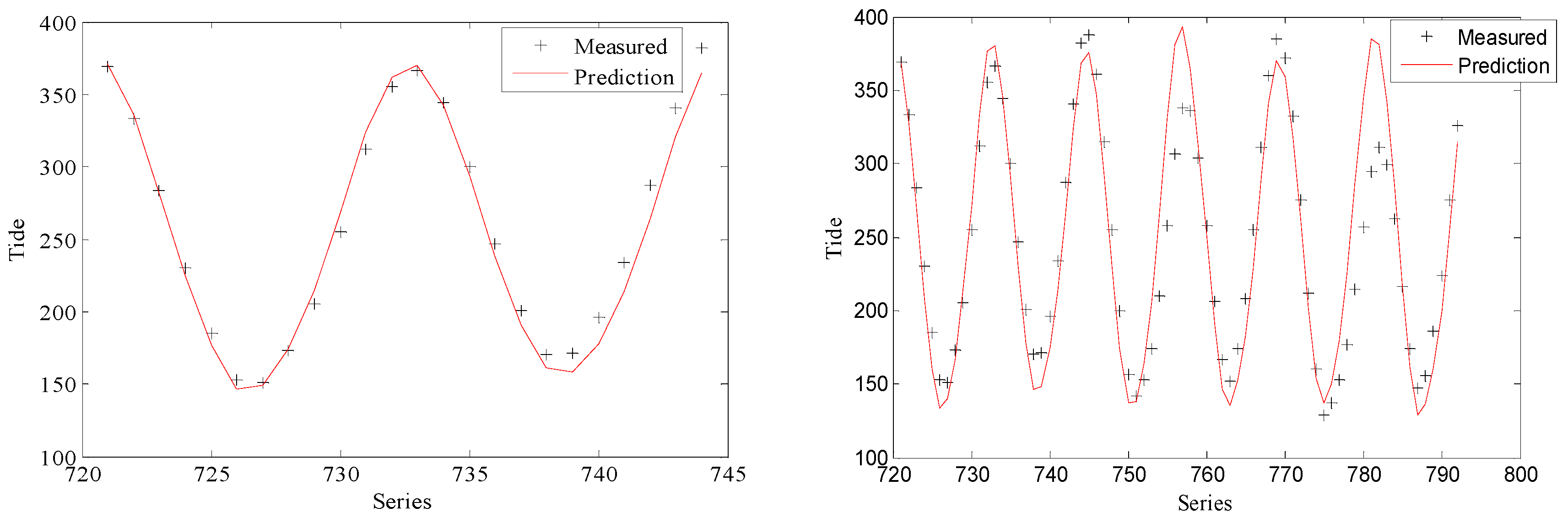
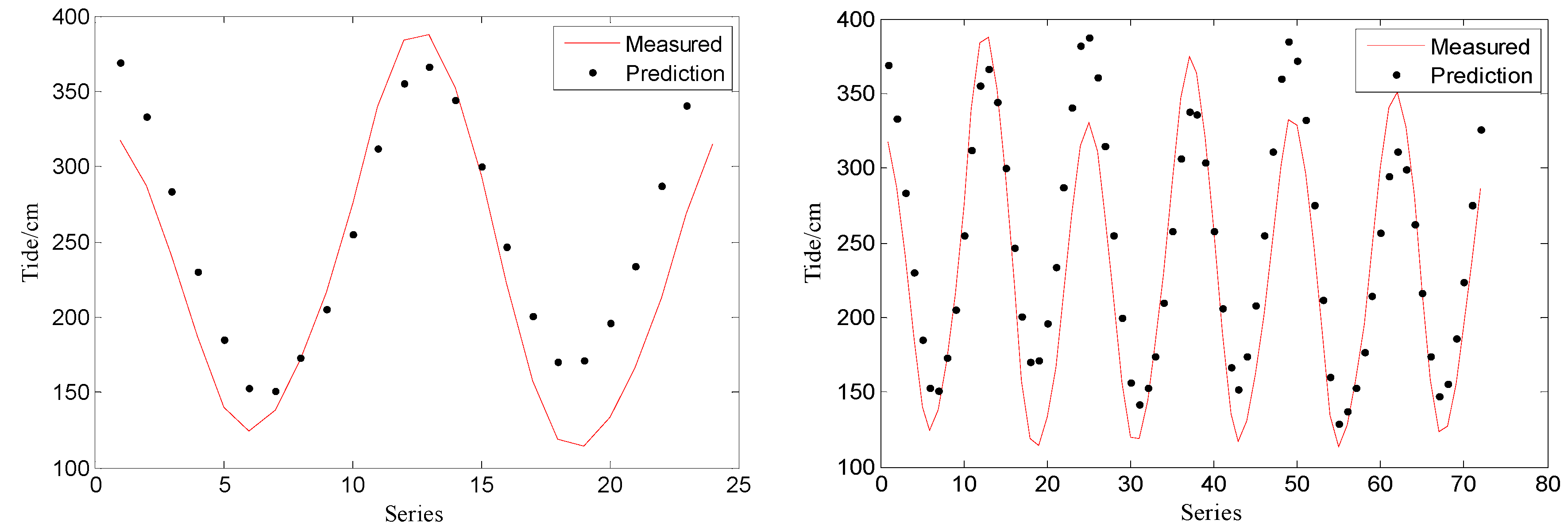
3.3. Prediction Results and Discussions

In view of the time-delay phenomenon existing in the neural network tidal prediction methods, the paper proposes a periodic analysis method, and uses the existing tidal data of one month to predict tide data in the next 24 and 72 h.
Figure 3 shows the response of output element for data series; we can see that the predicted values are in good agreement with the actual observations. The error values are mostly in the range of −5 to 5 cm, with some points exceeding ±10 cm. Relative to the observed data, the error is roughly within 5%.
Figure 4 is the auto correlation of error in lag 0–20, and the auto correlation at lag 0 is equal to the mean squared error. So, we can know that the mean squared error is only 9.4 cm2, which indicates the predicted results agree well with the measured results
Figure 5 is the predicted tide values for 24 h and 72 h, calculated by using multi-level iterative neural network in which the correlation between the 24 h predicted results and the measured results is 0.9965, and the correlation between the 72 h predicted results and the measured results is 0.9353. This means that for short-term forecasting, the prediction results of the method provided in this paper have good applicability. Additionally, the accuracy of prediction gradually decreases with the increase of prediction time. Therefore, the prediction results of this study have limitations. We also made one-day and three-day tidal predictions without iteration, and the correlation results were 0.9152 and 0.8646, respectively. It is clear that prediction accuracy without iteration is greatly reduced, especially for 3-day forecasts.
The harmonic analysis method is to calculate the harmonic constants of the local tide and to predict the tide level. Table 3 shows the amplitudes and phase lags of different tidal components based on harmonic analysis. Figure 6 shows the difference between actual values and predicted values based on harmonic constants. The correlation between the measured and actual values for 1 day is 0.9173, and it is 0.9230 for 3 days. It can be seen that the accuracy of tidal prediction value obtained by harmonic constant is less than the prediction result of neural network.

4. Discussion

With the continuous development of science and technology, people begin to shift their attention from land research to marine research. Among them, tidal observation can help coastal cities to predict weather in advance and can also provide marine environment forecast for the development of marine resources. In the traditional tide observation, a large number of research has started to use intelligent algorithms for prediction. With the continuous development of artificial intelligence technology, how to apply it to tide prediction has become the current focus of research. In the study, it is believed that the tide data has certain rules, but the time delay in it makes it difficult for most intelligent algorithms to achieve accurate tide prediction in application. Therefore, in the study, the adaptive ability of the BP neural network is used to periodically analyze the tide data and to improve the accuracy of the tide prediction.
In the research, the BP neural network is used to build a tidal time series prediction model, aiming to use the tidal values at different times to build a tidal prediction model, and to predict the future tidal values. The result shows that the error of tidal data prediction is controlled within 5%. Previous studies have shown that the use of neural networks can fully consider the weather conditions in the ocean, so the tidal data prediction can be controlled within a reasonable range, which is consistent with the results of this study [41]. The research results show that the lag error of time series prediction model combined with BP neural network is small, which is similar to the actual results. In previous studies, it was proposed to use BP neural network to predict ocean temperature. The use of time series data of ocean temperature can effectively improve the prediction accuracy of the model, which is consistent with the low lag results shown in the study [42]. In addition, in order to understand the similarity between the tidal prediction results and the actual values, a correlation analysis was conducted. The results show that the correlation coefficients between the predicted values and the actual values are above 0.9, which is consistent with the opinions put forward in previous studies [43].
To sum up, a BP neural network can show more effective prediction ability in tidal prediction, and the difference between the predicted value and the actual value is not significant. However, from the experimental results, it can be found that the prediction accuracy gradually decreases with the increase of prediction time because the prediction model in the study takes less account of other factors in the ocean, and other factors that affect the tides in the ocean need to be taken into account in further research to improve the comprehensiveness of the prediction model.

5. Conclusions

In this paper, the neural network BP algorithm is used to predict the tide time series. Considering the periodicity of tides, periodic analysis and data training are carried out in this paper. The results show that the prediction results after periodic analysis well solve the time delay problem, and improve the prediction accuracy of the network.
Compared with the traditional harmonic analysis method, the artificial neural network method has the advantage of fewer requirements on the measured data, which can use the limited measured data to predict with high accuracy. In actual work, the marine engineering construction department has an important demand for tide level prediction. Although this study can only provide an accurate forecast for 3 days, it is enough to deal with risks. How to improve the accuracy of long-term prediction is one of the future research directions.

Author Contributions

Conceptualization, H.S. and H.X.; methodology, H.X.; software, S.N.; validation, H.S., H.X. and S.N.; formal analysis, H.X.; writing—original draft preparation, H.X.; writing—review and editing, H.S.; visualization, H.X. All authors have read and agreed to the published version of the manuscript.

Funding

The authors gratefully acknowledge the support of the National Key R&D Program of China (Grant No.: 2018YFB1501901); the Natural Science Foundation of China (No. 51909114) and the Major Research Grant (No.:U1806227, U1906231) from the Natural Science Foundation of China (NSFC).

Institutional Review Board Statement

Not applicable.

Informed Consent Statement

Not applicable.

Data Availability Statement

Data are available from the corresponding author upon reasonable request.

Conflicts of Interest

The authors declare no conflict of interest.

References

  1. Chen, Z.Y. Tidology; Science Press: Beijing, China, 1980; pp. 5–9. [Google Scholar]
  2. Darwin, G. On an Apparatus for Facilitating the Reduction of Tidal Observations. Proc. R. Soc. Lond. 1892, 52, 345–389. [Google Scholar]
  3. Doodson, A.T. The analysis of tidal observations. Philos. Trans. R. Soc. A Math. Phys. Eng. Sci. 1928, 227, 223–279. [Google Scholar]
  4. Doodson, A.T. The analysis and predictions of tides in shallow water. Int. Hydrogr. Rev. 1957, 33, 85–126. [Google Scholar]
  5. Grewal, M.S.; Andrews, A.P. Klaman Filtering; Theory and Practice Using Matlab, 2nd ed.; Wiley: New York, NY, USA, 2001. [Google Scholar]
  6. Yen, P.H.; Jan, C.D.; Lee, Y.P.; Lee, H.F. Application of Kalman filter to short-term tide level prediction. J. Waterw. Port Coast. Ocean Eng. 1996, 122, 226–231. [Google Scholar] [CrossRef]
  7. Zhang, Z.; Luo, C.; Zhao, Z. Application of probabilistic method in maximum tsunami height prediction considering stochastic seabed topography. Nat. Hazards 2020, 104, 2511–2530. [Google Scholar] [CrossRef]
  8. Zhang, Y.; Liu, F.; Fang, Z.; Yuan, B.; Zhang, G.; Lu, J. Learning from a complementary-label source domain: Theory and algorithms. IEEE Trans. Neural Netw. Learn. Syst. 2021, 1–15. [Google Scholar] [CrossRef]
  9. Meng, F.; Xiao, X.; Wang, J. Rating the crisis of online public opinion using a multi-level index system. Int. Arab J. Inf. Technol. 2022, 19, 597–608. [Google Scholar] [CrossRef]
  10. Xie, W.; Li, X.; Jian, W.; Yang, Y.; Liu, H.; Robledo, L.F.; Nie, W. A novel hybrid method for landslide susceptibility mapping-based geodetector and machine learning cluster: A case of Xiaojin county, China. ISPRS Int. J. Geo-Inf. 2021, 10, 93. [Google Scholar] [CrossRef]
  11. French, M.N.; Krajewski, W.F.; Cuykendall, R.R. Rainfall forecasting in space time using a neural network. J. Hydrol. 1992, 137, 1–31. [Google Scholar] [CrossRef]
  12. Tsai, C.-P.; Lee, T.-L. Back-propagation neural network in tidal-level forecasting. J. Waterw. Port Coast. Ocean Eng. 1999, 125, 195–202. [Google Scholar] [CrossRef]
  13. Chen, B.F.; Chun, C.C.; Wang, D. Tide forecasting of tides around Taiwan by artificial neural network method and wavelet analysis. China Ocean Eng. 2007, 21, 659–675. [Google Scholar]
  14. Liu, C.; Yin, J.C. A high-precision short-term tide prediction model. J. Shanghai Marit. Univ. 2016, 037, 74–80. [Google Scholar]
  15. Qin, S.Y.; Li, J.J.; Long, B.X.; Zhang, Z.Y.; Wang, L.Z.; Yan, Y.H.; Sun, J.L. Tide tide prediction based on GPOS-BP neural networks. Mar. Inf. 2020, 2, 1–5. (In Chinese) [Google Scholar]
  16. Xu, D.J. An improved PSO-BP neural network red tide prediction model based on principal component analysis. Bull. Surv. Mapp. 2021, (Suppl. S2), 234–240. [Google Scholar]
  17. Di Nunno, F.; de Marinis, G.; Gargano, R.; Granata, F. Tide prediction in the Venice Lagoon using nonlinear autoregressive exogenous (NARX) neural network. Water 2021, 13, 1173. [Google Scholar] [CrossRef]
  18. Granata, F.; Di Nunno, F. Artificial Intelligence models for prediction of the tide level in Venice. Stoch. Environ. Res. Risk Assess. 2021, 35, 2537–2548. [Google Scholar] [CrossRef]
  19. Lee, T.L.; Jeng, D.S. Aplication of artificil ncural netwarks in tide forecting. Ocean Eng. 2002, 29, 1003–1022. [Google Scholar] [CrossRef]
  20. Wu, W.H.; Li, L.B.; Yin, J.C.; Lyu, W.Y.; Zhang, W.J. A modular tide level prediction method based on a NARX neural network. IEEE Access 2021, 9, 147416–147429. [Google Scholar] [CrossRef]
  21. Zhu, G.Q. Research on short-term tide forecast based on Bi-LSTM recurrent neural network. Int. J. Soc. Sci. Educ. Res. 2020, 3, 19–29. [Google Scholar]
  22. Tsai, C.P.; Lin, C.; Shen, J.N. Nenral nework for wave forecasting among muli-staions. Ocean Eng. 2002, 29, 1683–1695. [Google Scholar] [CrossRef]
  23. Haykin, S. Principles of Neural Networks; Mechanical Machinery Industry Press: Beijing, China, 2004. [Google Scholar]
  24. Xie, W.; Nie, W.; Saffari, P.; Robledo, L.F.; Descote, P.; Jian, W. Landslide hazard assessment based on Bayesian optimization–support vector machine in Nanping City, China. Nat. Hazards 2021, 109, 931–948. [Google Scholar] [CrossRef]
  25. Li, A.; Masouros, C.; Swindlehurst, A.L.; Yu, W. 1-Bit massive MIMO transmission: Embracing interference with symbol-level precoding. IEEE Commun. Mag. 2021, 59, 121–127. [Google Scholar] [CrossRef]
  26. Luo, G.; Zhang, H.; Yuan, Q.; Li, J.; Wang, F. ESTNet: Embedded spatial-temporal network for modeling traffic flow dynamics. IEEE Trans. Intell. Transp. Syst. 2022, 23, 19201–19212. [Google Scholar] [CrossRef]
  27. Yin, L.; Wang, L.; Huang, W.; Tian, J.; Liu, S.; Yang, B.; Zheng, W. Haze grading using the convolutional neural networks. Atmosphere 2022, 13, 522. [Google Scholar] [CrossRef]
  28. Yin, L.; Wang, L.; Zheng, W.; Ge, L.; Tian, J.; Liu, Y.; Liu, S. Evaluation of empirical atmospheric models using swarm-c satellite data. Atmosphere 2022, 13, 294. [Google Scholar] [CrossRef]
  29. Tian, J.; Liu, Y.; Zheng, W.; Yin, L. Smog prediction based on the deep belief—BP neural network model (DBN-BP). Urban Clim. 2022, 41, 101078. [Google Scholar] [CrossRef]
  30. Yao, L.; Li, X.; Zheng, R.; Zhang, Y. The impact of air pollution perception on urban settlement intentions of young talent in China. Int. J. Environ. Res. Public Health 2022, 19, 1080. [Google Scholar] [CrossRef]
  31. Liang, X.; Luo, L.; Hu, S.; Li, Y. Mapping the knowledge frontiers and evolution of decision making based on agent-based modeling. Knowl.-Based Syst. 2022, 250, 108982. [Google Scholar] [CrossRef]
  32. Xiong, Q.; Chen, Z.; Huang, J.; Zhang, M.; Song, H.; Hou, X.; Feng, Z. Preparation, structure and mechanical properties of Sialon ceramics by transition metal-catalyzed nitriding reaction. Rare Met. 2020, 39, 589–596. [Google Scholar] [CrossRef]
  33. Li, M.C.; Liang, S.X.; Sun, Z.C. Application of artificial neural networks to tide forecasting. J. Dalian Univ. Technol. 2007, 47, 101–105. [Google Scholar]
  34. Lin, W.; Yi, Z.; Tao, C. Back propagation neural network with adaptive differential evolution algorithm fortime series forecasting. Expert Syst. Appl. 2015, 42, 855–863. [Google Scholar]
  35. Kavzoglu, T.; Mather, P.M. The use of backpropagating artificial neural networks in land cover classification. Int. J. Remote Sens. 2003, 24, 4907–4938. [Google Scholar] [CrossRef]
  36. Hornik, K.; Stinchcombe, M.; White, H. Multilayer feedforward networks are universal approximators. Neural Netw. 1989, 2, 359–366. [Google Scholar] [CrossRef]
  37. Hornik, K. Approximation cupabilities of multilayer feedforward networks. Neural Netw. 1991, 4, 251–257. [Google Scholar] [CrossRef]
  38. Wen, X.H.; Chen, K.Z. A nonlinear time-series model based on a neural network. J. Xidian Univ. 1994, 1, 73–78. [Google Scholar]
  39. Lee, J.W.; Irish, J.L.; Bensi, M.T.; Marcy, D.C. Rapid prediction of peak storm surge from tropical cyclone track time series using machine learning. Coast. Eng. 2021, 170, 104024. [Google Scholar] [CrossRef]
  40. Liang, S.X.; Li, M.C.; Sun, Z.C. Prediction models for tidal level including strong meteorologic effects using a neural network. Ocean Eng. 2008, 35, 666–675. [Google Scholar] [CrossRef]
  41. Nunno, F.D.; Granata, F.; Gargano, R.; de Marinis, G. Forecasting of extreme storm tide events using NARX neural network-based models. Atmosphere 2021, 12, 512. [Google Scholar] [CrossRef]
  42. Wu, Z.; Jiang, C.; Conde, M.; Deng, B.; Chen, J. Hybrid improved empirical mode decomposition and BP neural network model for the prediction of sea surface temperature. Ocean Sci. 2019, 15, 349–360. [Google Scholar] [CrossRef] [Green Version]
  43. Zhang, X. Analysis of financial market trend based on autoregressive conditional heteroscedastic model and BP neural network prediction. J. Intell. Fuzzy Syst. 2020, 39, 5845–5857. [Google Scholar] [CrossRef]
Figure 1. The location of data observation.
Atmosphere 13 01999 g001
Figure 2. Schematic diagram of the data acquisition.
Atmosphere 13 01999 g002
Figure 3. The response of output element for data series.
Atmosphere 13 01999 g003
Figure 4. The auto correlation of error in lag 0–20.
Atmosphere 13 01999 g004
Figure 5. The predicted tide values of 24 h (left) and 72 h (right).
Atmosphere 13 01999 g005
Figure 6. The difference between actual values and predicted values based on harmonic constants for 24 h (left) and 72 h (right).
Atmosphere 13 01999 g006
Table 1. Effect of number of hidden layers on forecasting precision.
Hidden LayersPrediction ErrorNumber of Cycle StepsFitting Error
one0.009101645<0.005
two0.011305139
Table 2. Effect of node number of hidden layer on forecasting precision.
Number of NodesPrediction ErrorNumber of Cycle StepsFitting Error
60.00861586635<0.005
70.00810531440
80.00923457471
Table 3. Results of four tidal components obtained by harmonic analysis.
TideFrequencyAmplitudePhase LagsTideFrequencyAmplitudePhase Lags
M20.08178.1694.86S20.08343.98119.05
O10.03938.31173.66K10.04232.01218.63
Publisher’s Note: MDPI stays neutral with regard to jurisdictional claims in published maps and institutional affiliations.

