Article

Short-Term Rainfall Prediction Based on Radar Echo Using an Improved Self-Attention PredRNN Deep Learning Model

1
State Key Laboratory of Plateau Ecology and Agriculture, Department of Computer Technology and Applications, Qinghai University, Xining 810016, China
2
Brookhaven National Laboratory, Upton, NY 11973, USA
*
Author to whom correspondence should be addressed.
Atmosphere 2022, 13(12), 1963; https://doi.org/10.3390/atmos13121963
Submission received: 1 September 2022 / Revised: 20 November 2022 / Accepted: 22 November 2022 / Published: 24 November 2022

Abstract

:
Accurate short-term precipitation forecast is extremely important for urban flood warning and natural disaster prevention. In this paper, we present an innovative deep learning model named ISA-PredRNN (improved self-attention PredRNN) for precipitation nowcasting based on radar echoes on the basis of the advanced PredRNN-V2. We introduce the self-attention mechanism and the long-term memory state into the model and design a new set of gating mechanisms. To better capture different intensities of precipitation, the loss function with weights was designed. We further train the model using a combination of reverse scheduled sampling and scheduled sampling to learn the long-term dynamics from the radar echo sequences. Experimental results show that the new model (ISA-PredRNN) can effectively extract the spatiotemporal features of radar echo maps and obtain radar echo prediction results with a small gap from the ground truths. From the comparison with the other six models, the new ISA-PredRNN model has the most accurate prediction results with a critical success index (CSI) of 0.7001, 0.5812 and 0.3052 under the radar echo thresholds of 10 dBZ, 20 dBZ and 30 dBZ, respectively.

1. Introduction

Precipitation prediction is one of the most important meteorological services. In particular, short-term precipitation forecasting is more closely related to many aspects of people’s lives. Short-term precipitation forecast generally refers to predicting the precipitation intensity in the next 0–2 h. It is highly time-sensitive. Precise short-term precipitation forecasting is of great practical significance, making travel easier, guiding agricultural production and preventing and mitigating disaster.
At present, numerical weather prediction (NWP) and radar echo extrapolations are the two mainstream methods of precipitation forecasting. Numerical weather prediction-based methods perform future precipitation forecasting by solving complex physically based prognostic weather equations. However, numerical weather prediction has the drawbacks of uncertainty and parametric errors, and generates large computational overhead in solving mathematical equations, which is more suitable for medium and long-term precipitation prediction. The radar echo extrapolation-based method uses previous radar echo sequences to extrapolate future radar echo sequences and thus make precipitation forecasts for future periods. Currently, monomeric center-of-mass-based methods, mutual correlation-based methods, and optical flow-based methods are widely used in radar echo weather forecasting. The single-body center-of-mass-based approach is suitable for tracking isolated, large, strong echoes of single bodies or groups of single bodies. Dixon et al. [1] used the method for identification, tracking, analysis and proximity forecasting of thunderstorms on radar echo maps. The intercorrelation-based approach uses the best spatial correlation of different regions of adjacent time radar echoes to infer the location of future radar echoes, such as Liang et al. [2] combining the intercorrelation-based approach with model predicted winds for radar echo extrapolation. The optical flow approach is a method in the field of computer vision that is also applied to weather forecasting due to its good motion tracking capability. Zhu et al. [3] used this method for tropical cyclone precipitation forecasting. However, radar echo has no obvious periodicity, and it does not move at a fixed rate or have a fixed pattern of shape change. Radar echoes in different weather scatter, merge and split over time, and also has the evolution of generation and elimination to some extent. This poses challenges to accurate radar echo precipitation forecasting using the traditional methods described above.
In recent years, with the development of artificial intelligence, machine learning methods are being used more and more widely. Many machine learning-based models have shown great advantages for applications in the field of meteorology. Yang et al. [4] proposed the terrain-based weighted random forests (TWRF) method, which improved the accuracy of radar quantitative precipitation estimation. Bhuiyan et al. [5] proposed the nonparametric statistical model based on quantile regression forests (QRF) for modeling rainfall retrieval error. Zhang et al. [6] proposed a novel double machine learning (DML) approach to merge multiple satellite-based precipitation products (SPPs) and gauge observations. Banadkooki et al. [7] obtained precipitation maps highly consistent with the observed values using support vector machine optimization based on the flow regime algorithm for precipitation forecasting. Chiang et al. [8] proposed a Bayesian merging with gamma distribution (BMG) to solve discontinuous problems in rainfall assimilation under more practical rainfall distribution. Kolluru et al. [9] used machine learning (SPEM2L) algorithms for merging multiple global precipitation datasets to improve spatiotemporal rainfall characterization. Compared with traditional machine learning methods, deep learning models use deeper network structures that are suitable for modeling complex dependencies. The application of deep learning methods in the field of meteorology has not only led to more accurate weather forecasting results, but also significantly reduced the computational cost and processing time before forecasting. The feature exactly meets the requirements of real-time and accuracy of short-term forecasting.
Weather forecasting can be seen as a sequential problem from the temporal perspective, i.e., using the weather conditions of a past period to predict the weather conditions of a future period. The circular structure of recurrent neural networks (RNNs) is well suited to dealing with sequential problems [10,11,12,13,14,15]. Convolutional neural networks (CNNs) are more suitable for capturing spatial location information, which is often used to process various pieces of image information [16,17,18,19,20,21]. Since many weather conditions involve both temporal and spatial factors, the combination of RNNs and CNNs is often used for weather prediction in order to better capture spatiotemporal correlations. Shi et al. [22] first combined CNN with RNN to design the convolutional long short-term memory (ConvLSTM) network for short-term precipitation forecasting in Hong Kong using a radar echo dataset, which is gradually used in various scenarios of weather forecasting for the better combination capability of location and sequence information [23,24,25]. Trajectory gated recurrent unit (TrajGRU) [26] is another network for spatiotemporal prediction developed on the basis of ConvLSTM, which has better motion feature extraction ability and more accurate radar echo prediction results. Wang et al. [27] proposed the predictive recurrent neural network (PredRNN) based on the spatiotemporal memory unit Spatiotemporal LSTM (ST-LSTM), which can be seen as a combination of two ConvLSTM basic units stacked up and down, with the upper part called the standard temporal memory structure and the lower part called the spatiotemporal memory structure. The structure of the ST-LSTM cell enables it to process spatiotemporal information better. In addition, the overall network architecture of PredRNN enhances the utilization of visual features by adding hidden states of zigzag transmission, which is a spatiotemporal state flowing through each node of the entire network. As a result, compared with previous work, PredRNN is able to obtain higher quality extrapolation images in prediction. PredRNN-V2 [28] adds a new decoupling loss to the basic structural unit of the original PredRNN, which allows the upper and lower parts of the ST-LSTM structure to focus on different aspects of spatiotemporal variation better.
However, the radar echo maps obtained from the predictions of many current deep learning models are rather blurred. In order to obtain clearer radar echo maps, many studies have incorporated generative adversarial networks (GANs) into various deep learning models for weather forecasting. The GAN consists of two modules, the generative model and the discriminative model. It generates detail-rich image results through adversarial learning. Xu et al. [29] used the GAN-LSTM model for satellite image prediction and obtained better results than the traditional autoencoder-LSTM network. Singh et al. [30] proposed a GAN-based discriminator loss based on the ConvLSTM network structure, which predicts radar echo maps with high accuracy. Although the application of GAN can make the predicted radar echo maps more clear, it tends to lead to the generated results containing some false detailed information. This affects the accuracy of the forecast results.
The development of an attention mechanism has injected new vitality into artificial intelligence. It has achieved excellent results in applications such as image recognition [31,32,33,34,35], target detection [36,37,38,39], and natural language processing [40,41]. As the attention mechanism flourishes in various fields, it is gradually being introduced into the meteorological field to reduce forecast errors. Lin et al. [42] introduced a channel-wise attention mechanism that adaptively scales each simulation parameter to maximize useful information when using dual-source spatiotemporal neural networks for lightning forecasting. Yan et al. [43] incorporated the multi-head attention into a dual-channel neural network to enhance the model’s focus on precipitation forecasting in critical regions. Sønderby et al. [44] introduced an axial self-attention to the meteorological neural network (MetNet) architecture and achieved better results than numerical weather prediction for precipitation forecasting on the scale of the continental United States.
In order to capture the long-term and short-term spatiotemporal correlations better, enhance the accuracy of the model for extreme precipitation forecasting, and narrow the gap between training and inference processes, we propose to improve the PredRNN by using improved self-attention in this paper. In this model, the attention mechanism is incorporated inside the ST-LSTM to generate a new ISA-LSTM spatiotemporal memory unit, which provides better access to global feature information and long-term memory information and is more effective in focusing on different aspects of spatiotemporal changes. A loss function with different weights for different precipitation intensity was designed, so that the model could capture extreme precipitation better. We used the combination of reverse scheduled Sampling and Scheduled Sampling as the training strategy for the model. It promotes the learning of the long-term dynamics in the sequence and narrows the gap between training and inference processes. The new model organically combines the above methods that contribute to the accuracy of the prediction results and avoids the drawbacks of GAN while obtaining more clear radar echo images.
Satellite datasets and radar echo datasets are commonly used for precipitation forecasting. Meteorological satellites are developing rapidly and can monitor the Earth in all directions. Although the satellite provides a wide range of optical observation capabilities, it has a low resolution of cloud maps. The satellite dataset is suitable for large scale, less resolution-demanding prediction tasks [45,46]. Radar has a limited coverage area and can be used for real-time detection of small-scale weather processes in local areas. The radar echo dataset is suitable for prediction tasks with smaller ranges and higher resolutions [47,48]. Since the study in this paper focuses on short-term precipitation forecasting over the small region, we used the radar echo dataset for the experiment. Our ISA-PredRNN model works best when evaluated on the radar echo dataset. Therefore, the application of the new model is effective in improving the accuracy of short-term rainfall prediction.
The remainder of this paper is organized as follows: In Section 2, the method of data denoising is described, and the process of preparing the dataset is presented. In Section 3, the problem of short-term precipitation forecasting is described, and the method used in this paper is presented in detail. The experimental results of the new method and several other mainstream models are compared and analyzed in Section 4. Finally, a summary of the paper is presented in Section 5.

2. Data and Data Processing
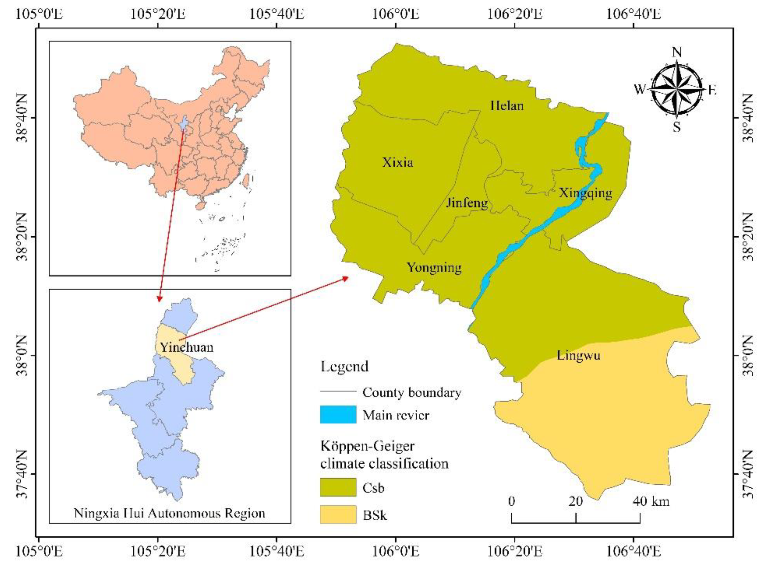
2.1. Study Area

Yinchuan City in the Ningxia Hui autonomous region was selected as the study region for this research. Ningxia is located in the northwestern part of the Loess Plateau in the middle and upper reaches of the Yellow River, and the climate type of the region is a continental semi-humid and semi-arid climate. The region is not only arid with little rainfall, but also has uneven spatiotemporal distribution of precipitation. Yinchuan is the political, economic and cultural center of Ningxia and straddles two climate zones, the warm summer Mediterranean climate (CSB) and the cool semi-arid climate (BSK). The location of the Ningxia Hui autonomous region and the Köppen climate classification of Yinchuan are shown in Figure 1. The main climatic characteristics of the region are scarce rain and snow and strong evaporation of water.

2.2. Data Cleaning

Radar beam propagation is easily interfered with by the surrounding mountains, buildings and dust, etc. This makes noise appear on the radar echo map. Insufficient calibration and damage to the measurement instrument can cause noise in the radar echo map. Deviations in the placement angle of the measuring instrument can also contribute to the noise. If training is conducted directly using the original radar maps, it makes the model difficult to converge with and leads to large forecast errors. In this paper, we follow Shi et al. [20] and categorize locations that have the Mahalanobis distances higher than the mean distance plus three times the standard deviation as outliers. These outliers were removed using the Mahalanobis denoising method. The original and denoised radar echo maps are shown in Figure 2. The process is as follows: First, the mean μ and covariance matrix S of all pixel points x 1 , x 2 , , x n on each image are calculated. Then, the Mahalanobis distance D M ( x ) of all pixel points is calculated. Finally, the points whose pixels are outliers are removed. This method can remove some discrete points caused by noise. The equations for calculating the Mahalanobis distance are shown as follows:
μ = i = 1 n x i n S = i = 1 n x i μ x i μ T n 1 D M ( x ) = ( x μ ) T S 1 ( x μ )

2.3. Preparation of Dataset

In order to verify the effectiveness of ISA-PredRNN in short-term precipitation forecasting from radar echo images, the two-year radar echo dataset from 2018 to 2019, obtained by gathering data every six minutes in Yinchuan, Ningxia was used for training and testing in this paper. The dataset was processed with data cleaning. Due to the small proportion of precipitation days among all days in the dataset, 84 days of precipitation data were selected to constitute the final dataset in this paper in order to prevent the network from treating precipitation conditions as noise and to enable the network to learn better. The original image contains 461 × 461 pixels, in order to facilitate the learning of the model and not to lose details, the image was cropped to a size of 200 × 200 containing the Yinchuan area of Ningxia in this paper. Since the extreme values of radar echoes in the dataset do not exceed 70 dBZ, the data were normalized by the calculation of z / 70 . Finally, in order to obtain enough sequences to allow adequate training of the model, a sliding window was used in this paper on daily radar echo data. Since the radar echo map is generated every 6 min and the proposed model can predict the precipitation in the next 1 h, the length of the sliding window was set to 20, with the first 10 frames used for learning and the last 10 frames used for prediction. In this paper, the training and test sets were divided evenly to a ratio of 4:1.

3. Methodology

3.1. Problem Definition
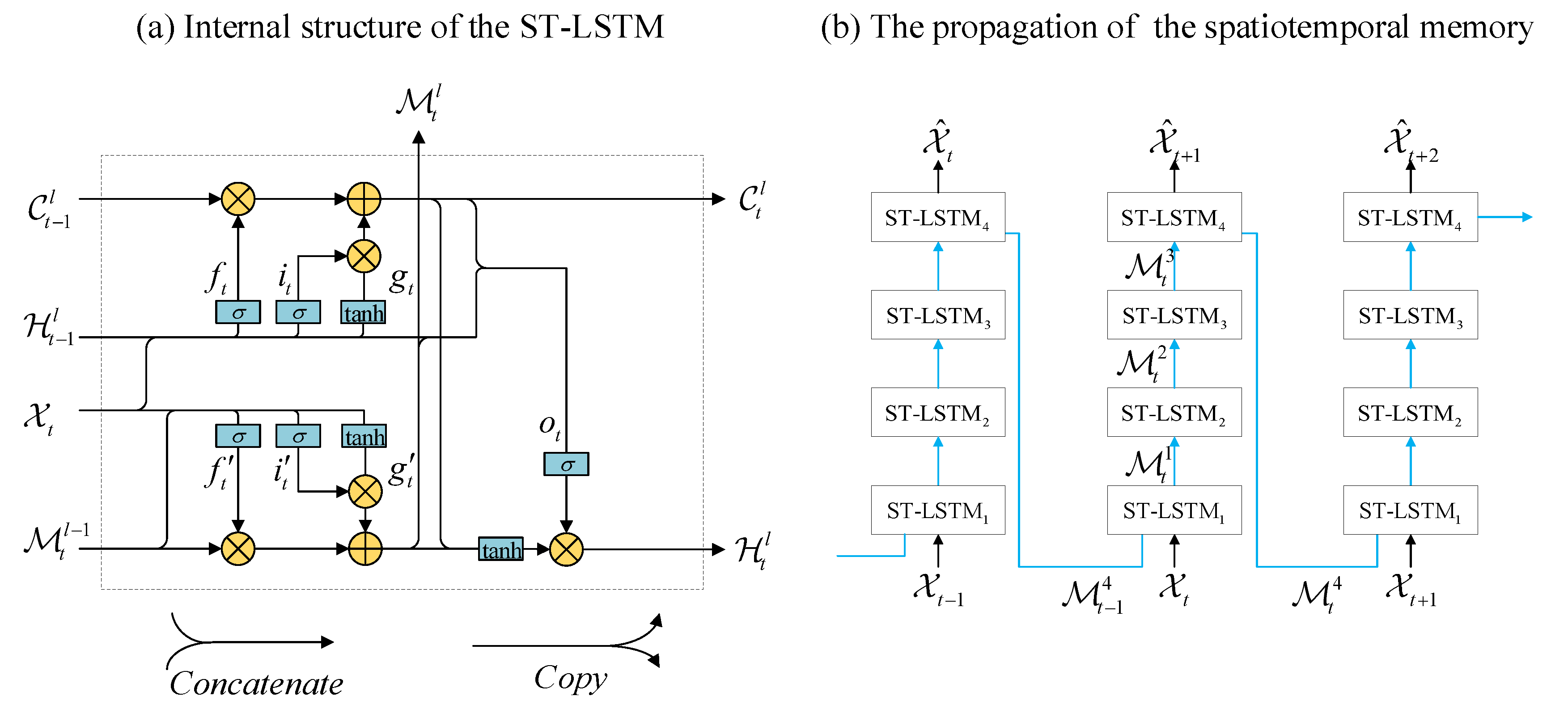
One method of short-term precipitation forecasting is to use radar echo maps from past periods to predict radar echo maps for future periods. Since the forecast is for precipitation over a period of time in a region, the problem involves both temporal and spatial factors. Specifically, a square image can be obtained by dividing the latitude and longitude range of an area with a certain spatial resolution. The pixel value of each grid point on the picture is the radar echo value of the place. The local precipitation can be calculated from the radar echo values. In this paper, we need to use multiple consecutive radar echo pictures in the past to infer multiple consecutive radar echo pictures in the future. This problem can be defined strictly in the following way: assuming the current time is t , we need to predict the radar echo sequence R t + 1 , R t + 2 , , R t + q of time length q in the future based on the radar echo sequence R t p + 1 , R t p + 2 , , R t of time length p in the past. The role of the model is to minimize the gap between the series R t + 1 , R t + 2 , , R t + q and the real future series R ˜ t + 1 , R ˜ t + 2 , , R ˜ t + q . This can be expressed as:
R t + 1 , R t + 2 , , R t + q = f θ R t p + 1 , R t p + 2 , , R t
where f denotes the precipitation forecast model and θ denotes the model parameters to be optimized.

3.2. Base Model

Short-term precipitation prediction means predicting the future precipitation of an area for a relatively short period of time in the future (e.g., 0–2 h). ConvLSTM can effectively combine temporal and spatial information and is more suitable for dealing with such problems. ConvLSTM is a model derived from LSTM. It uses the way of gate to control the retention, abandonment and refresh of information. ConvLSTM includes three gates: input gate, forgetting gate and output gate. The input gate controls the degree to which the current moment’s input X t is saved to the cell state C t . The forgetting gate controls the extent to which the cell state C t 1 at the previous moment is saved to the current moment C t . The output gate determines how much the cell state C t contributes to the current output value H t . The organic combination of the three gates allows the model to selectively remember the effective information and forget the disturbing information, avoiding the gradient disappearance and gradient explosion. The specific formulas of ConvLSTM are shown as follows:
i t = σ W x i X t + W h i H t 1 + W c i C t 1 + b i f t = σ W x f X t + W h f H t 1 + W c f C t 1 + b f C t = f t C t 1 + i t tanh W x c X t + W h c H t 1 + b c o t = σ W x o X t + W h o H t 1 + W c o C t + b o H t = o t tanh C t
where i t and f t denote the input gate and forget gate, respectively. o t denotes output gate. denotes the convolution operation. denotes Hadamard product. σ denotes sigmoid function. W before denote kernels for respective gates. W before denote the corresponding weight matrices. b denotes the bias value.
The basic constituent unit ST-LSTM of PredRNN can be regarded as a merger of two basic constituent units of ConvLSTM. The internal structure of the spatiotemporal memory unit ST-LSTM is shown in Figure 3a. There are two memory states inside the ST-LSTM cell. The first memory state C t is called standard time memory, which is transmitted inside ST-LSTM cells of adjacent time steps on the same layer. The second memory state M t is called spatiotemporal memory, which first propagates vertically upward between different layers of the same time step and then passes from the top layer of the previous moment to the first layer of the next moment. It reserves the abstract information extracted from each input through the multi-layer network structure for the next first layer, enhancing the network’s use of spatiotemporal information. The propagation of the spatiotemporal memory M t is shown in Figure 3b. The standard temporal memory state C t and the spatiotemporal memory state M t can facilitate long-term and short-term dependent learning processes, respectively, so that the network can make more effective use of spatiotemporal information. The specific formulas for the ST-LSTM cell are shown as follows:
g t = tanh W x g X t + W h g H t 1 l + b g i t = σ W x i X t + W h i H t 1 l + b i f t = σ W x f X t + W h f H t 1 l + b f C t l = f t C t 1 l + i t g t g t = tanh W x g X t + W m g M t l 1 + b g i t = σ W x i X t + W m i M t l 1 + b i f t = σ W x f X t + W m f M t l 1 + b f M t l = f t M t l 1 + i t g t o t = σ W x o X t + W h o H t 1 l + W c o C t l + W m o M t l + b o H t l = o t tanh W 1 × 1 C t l , M t l
The ST-LSTM cell introduces another set of gate structures for the spatiotemporal memory state M t while preserving part of the gate structures in ConvLSTM. M t propagates in a zigzag pattern throughout the network. l indicates at which layer of the network the corresponding state is located. The input gate i t , forget gate f t and input-modulation gate g t are the original gates in ConvLSTM. They control the information flow across the memory state C t . The functions of i t , f t and g t are the same as above, but they control the information flow across the memory state M t . The output gate o t is an improvement on the original output gate, which is shared by two memory states mentioned above. Finally, the final hidden state H t of this node originates from the fused spatiotemporal memory. The design of the ST-LSTM cell allows the model to effectively simulate shape changes and motion trajectories in spatiotemporal sequences.
During the operation of the PredRNN model, the memory states C t and M t are often intertwined, leading to inefficient utilization of the network parameters. A new decoupling loss function based on PredRNN is designed in PredRNN-V2, which increases the distance between C t and M t so that they focus on different aspects of spatiotemporal variation, respectively. The specific formulas for the decoupling loss function are shown as follows:
Δ C t l = W decouple   i t g t Δ M t l = W decouple   i t g t L decouple   = t l c Δ C t l , Δ M t l c Δ C t l c Δ M t l c
where W decouple   denotes 1 × 1 convolutions shared by all ST-LSTM cells. i t , g t , i t and g t can be calculated from Equation (4). Δ C t l and Δ M t l denote the increments of the two memory states, respectively. By defining the decoupling loss L decouple   in terms of the cosine similarity Δ C t l , Δ M t l c / Δ C t l c Δ M t l c , the PredRNN-V2 can effectively separate the two memory states.

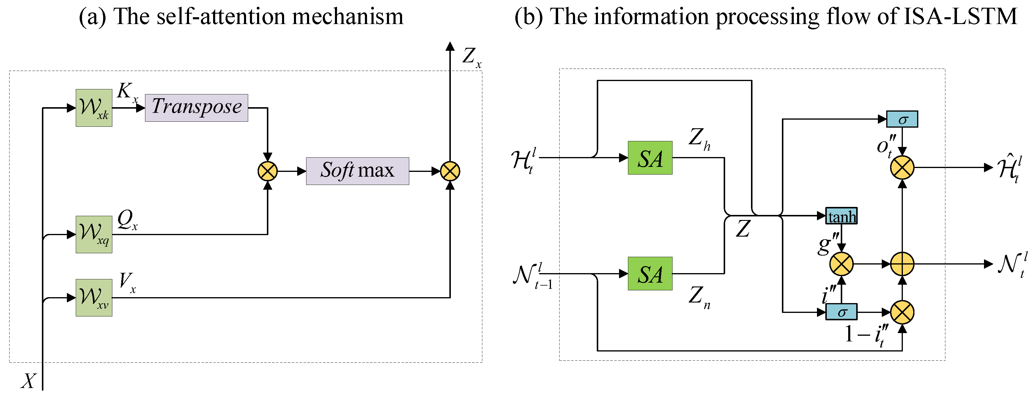
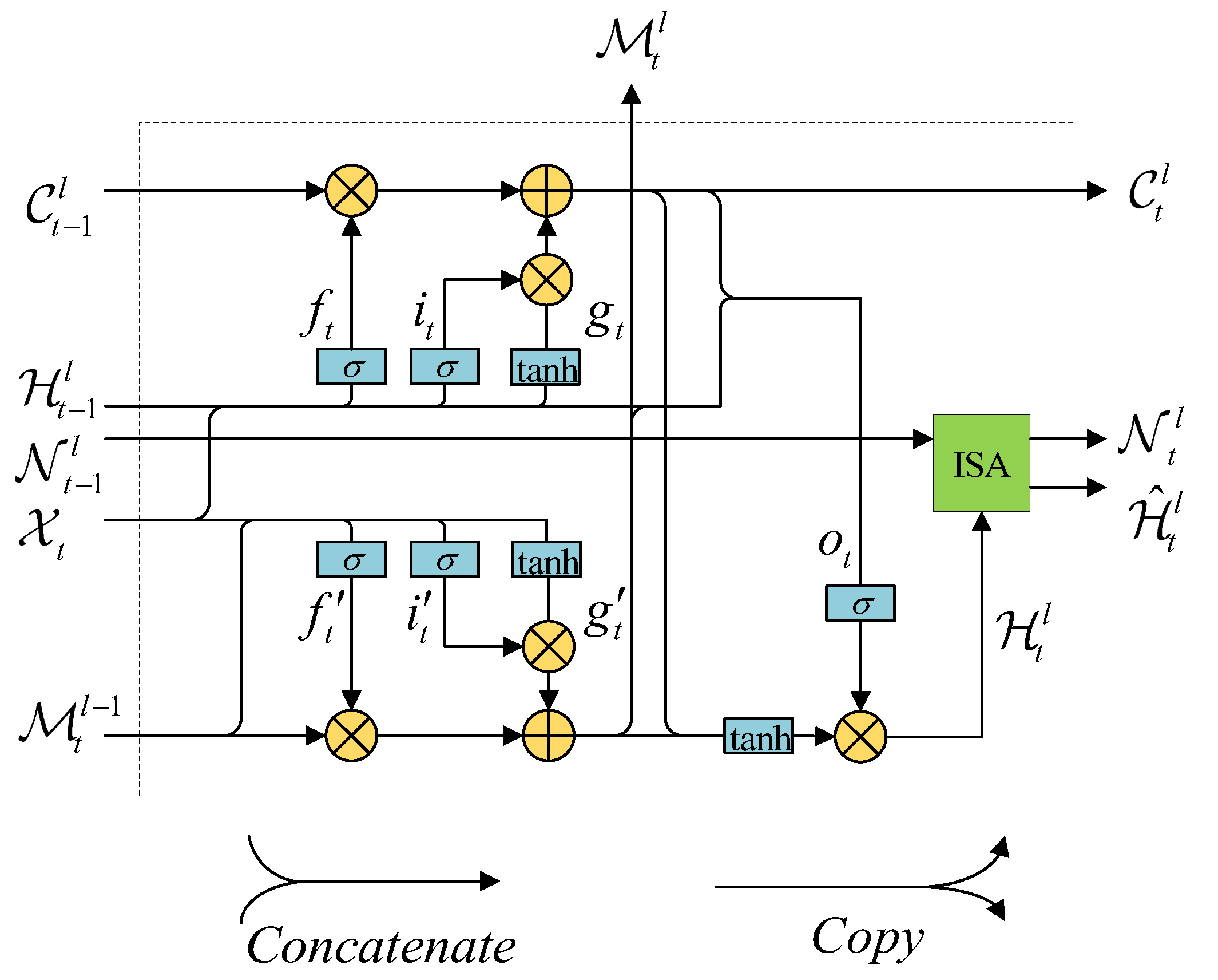
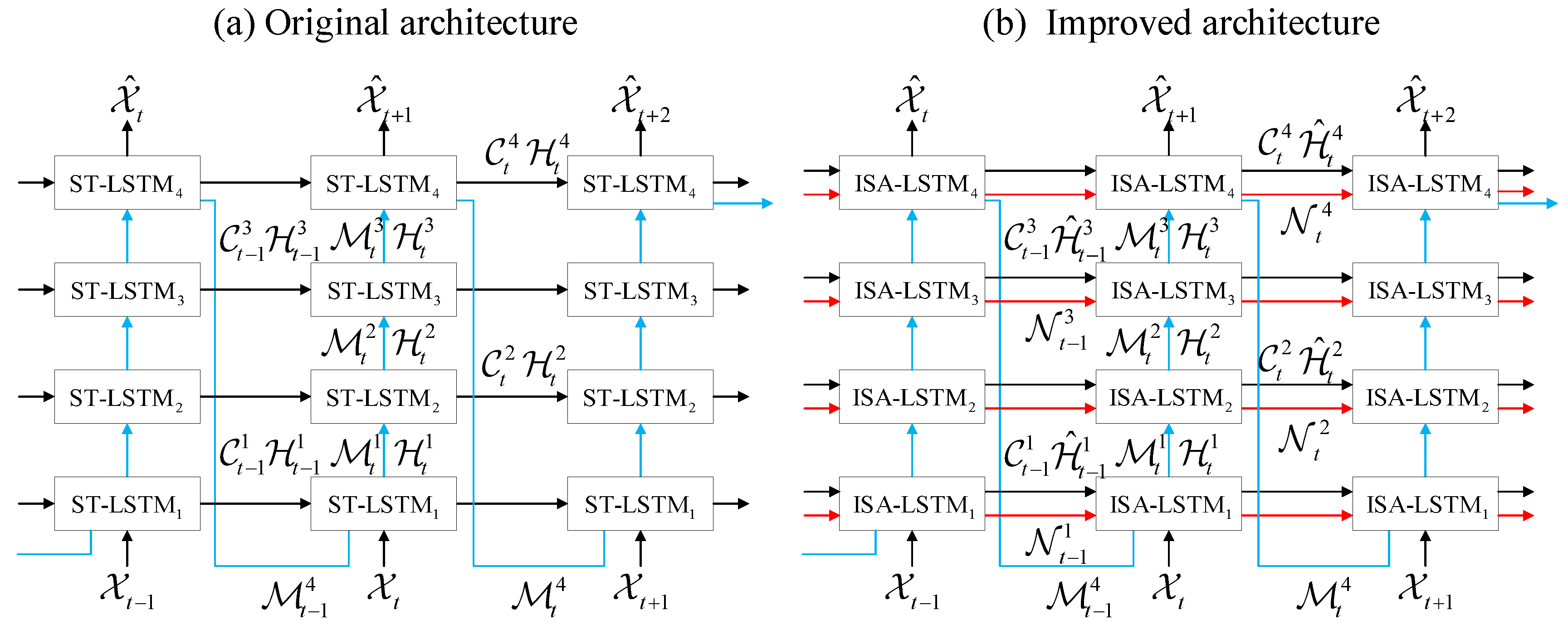
3.3. Improved Self-Attention PredRNN

ConvLSTM and its variants enable the model to focus on spatial information while processing temporal information by adding convolutional operations to the recurrent network. The PredRNN family is evolved from ConvLSTM, and its basic structural unit ST-LSTM can better handle the spatiotemporal correlation. However, the convolution operations in these models are suitable for handling local spatial information. In this paper, the self-attention mechanism was incorporated inside the ST-LSTM cell to enable the model to capture global spatial information better. The operation principle of the self-attention mechanism is shown in Figure 4a. The PredRNN family of networks enhances the ability of the model to learn short-term dependent information by introducing a spatiotemporal memory state M t inside the memory unit. In this paper, the long-term memory state N t was introduced into the memory unit, and a GRU-like update gate was designed. The new set of gate structures control the extent to which the previous moment’s memory state N t 1 is carried over to the current moment’s state N t , allowing the model to pay more attention to the long-term dependence. The internal structure of the new spatiotemporal memory unit ISA-LSTM is shown in Figure 5. The information processing flow of ISA-LSTM is as follows: First, the hidden state H t of the current moment and the long-term memory state N t 1 of the previous moment are passed through the self-attention module to extract the globally important information of these two states. Then, the hidden state, long-term memory state and the original hidden state obtained in the previous step are stitched in the channel dimension, and the stitched result is passed through a GRU-like update gate to obtain the long-term memory state N t at the current moment. Finally, the current long-term memory state N t and the generated splicing result are used to calculate the output hidden state H ^ t . The information processing flow of the ISA-LSTM is shown in Figure 4b, and the specific formulas of the ISA-LSTM cell are shown as follows:
Z h = W h v H t l S o f t max W h q H t l T W h k H t l Z n = W n v N t 1 l S o f t max W h q H t l T W n k N t 1 l Z = W z Z h , Z n i t = σ W z i Z + W h i H t l + b i g t = tanh W z g Z + W h g H t l + b g N t l = 1 i t N t 1 l + i t g t o t = σ W z o Z + W h o H t l + b o H ^ t l = o t N t l
where the intermediate features Z h and Z n are obtained by applying self-attention on the hidden state H t l and the previous moment memory state N t 1 l , respectively; the polymerization feature Z is obtained by aggregating the intermediate features Z h and Z n . i t , g t and o t are the input gate, input-modulation gate and output gate of the new set of gating mechanisms. N t l and H ^ t l are the final long-term memory states and hidden states.
The overall network architecture of the new model ISA-PredRNN proposed in this paper is shown in Figure 6b, and the network architecture of the original PredRNN-v2 is shown in Figure 6a. We borrowed the network architecture approach from PredRNN-v2, which uses a four-layer network structure. The difference is that we replaced all the basic structural units in the network with the ISA-LSTM. Among them, the newly introduced long-term memory state N t is one of the highlights of this network architecture.

3.4. Sampling Strategy

When using a sequential model for spatiotemporal prediction, the traditional approach works as follows. First, the true value is used as an input in the encoding phase and the generated value is obtained in the prediction phase. Then, based on the gap between the generated value and the true value at the same moment, the parameters of the model are updated by backpropagation of the gradient. Finally, it iterates in this way until the model is trained to a suitable state. However, only the real value is used in the coding process, which leads to the model not being able to exploit the non-Markovian nature of the historical observations better, and only the generated values are used in the prediction process, which leads to gaps in the training and inference process. In this paper, the model was trained using both reverse scheduled sampling and scheduled sampling. The data input to our model contains both ground truths and prediction values throughout the process. Specifically, the ground truths are input with increasing probability in the encoding phase and with decreasing probability in the prediction phase. The treatment in this paper allows the model to dig deeper into the non-Markovian properties of historical observations, capture the long-term dynamics in the sequence better, and also bridge the gap between the model training and inference process.

3.5. Improved Loss Function

When deep learning models are used for weather forecasting, the precipitation forecasting problem is often treated as an ordinary spatiotemporal forecasting problem. This treatment ignores the difference in the probability of occurrence of different intensities of precipitation in forecasting, which makes the forecast results less accurate. In order to fully consider the specific characteristics of the problem, we designed an improved loss function. According to the statistics, about 90% of precipitation is no larger than 0.5 mm/h, and no more than 1% of cases exceed 30 mm/h in our dataset. To capture the extreme precipitation better and make the forecast results more accurate, the weight loss function was designed in this paper. Specifically, since the precipitation intensity and the radar echo intensity are positively correlated and can be transformed by the Z-R relationship, we assigned different weights to the different radar echo intensities separately. Large weights were assigned to large echo intensities and small weights to small echo intensities. The specific weights were assigned as follows:
w ( z ) = 1 z < 20 2 20 z < 30 3 30 z ( dBZ )
where w ( z ) is the weight value corresponding to the radar echo intensity z at different thresholds. The final loss function can be expressed as follows:
L final = λ 1 L MSE + λ 2 L MAE + λ 3 L decouple  
where λ 1 , λ 2 and λ 3 control the relative importance. L MSE and L MAE are the MSE and MAE loss functions, respectively.

4. Results

4.1. Implementation Details

The implementation of the experiment is based on the PyTorch machine learning framework on NVIDIA GeForce GTX 1080 Ti GPUs. The CUDA version is 11.5 and the PyTorch version is 1.7. We compared the new ISA-PredRNN algorithm with six models, namely FC-LSTM, ConvLSTM, ConvGRU, TrajGRU, PredRNN-V2 and ISA-PredRNN (without weight loss) to verify its advancement. During the training process, the number of network layers of all the above seven models was set to four. The improved model has 128 convolutional kernels per layer of the network, a batch size of eight, a learning rate of 0.0001, an optimizer of Adam, and 80,000 iterations.

4.2. Evaluated Algorithm

To evaluate the performance of the improved algorithm, five metrics, probability of detection (POD), false alarm rate (FAR), critical success index (CSI), Heidke skill score (HSS), and mean square error (MSE), were used as the evaluation criteria for model effectiveness in this paper. In the field of precipitation prediction, since different degrees of precipitation conditions are given different levels of attention, the precipitation thresholds were divided into three levels of 10 dBZ, 20 dBZ and 30 dBZ according to the intensity of radar echoes in this paper, and the POD, FAR, CSI and HSS were calculated under each level. The four indicators of POD, FAR, CSI and HSS are formulated as follows:
POD = TP TP + FP FAR = FN TP + FN CSI = TP TP + FN + FP HSS = TP × TN FN × FP ( TP + FN ) ( FN + TN ) + ( TP + FN ) ( FP + TN )
where TP indicates prediction = 1 ,   truth = 1 , FP indicates prediction = 1 ,   truth = 0 , TN indicates prediction = 0 ,   truth = 0 and FN indicates   prediction = 0 ,   truth = 1 . The lower the FAR, the higher the POD, CSI and HSS, the better the model prediction.

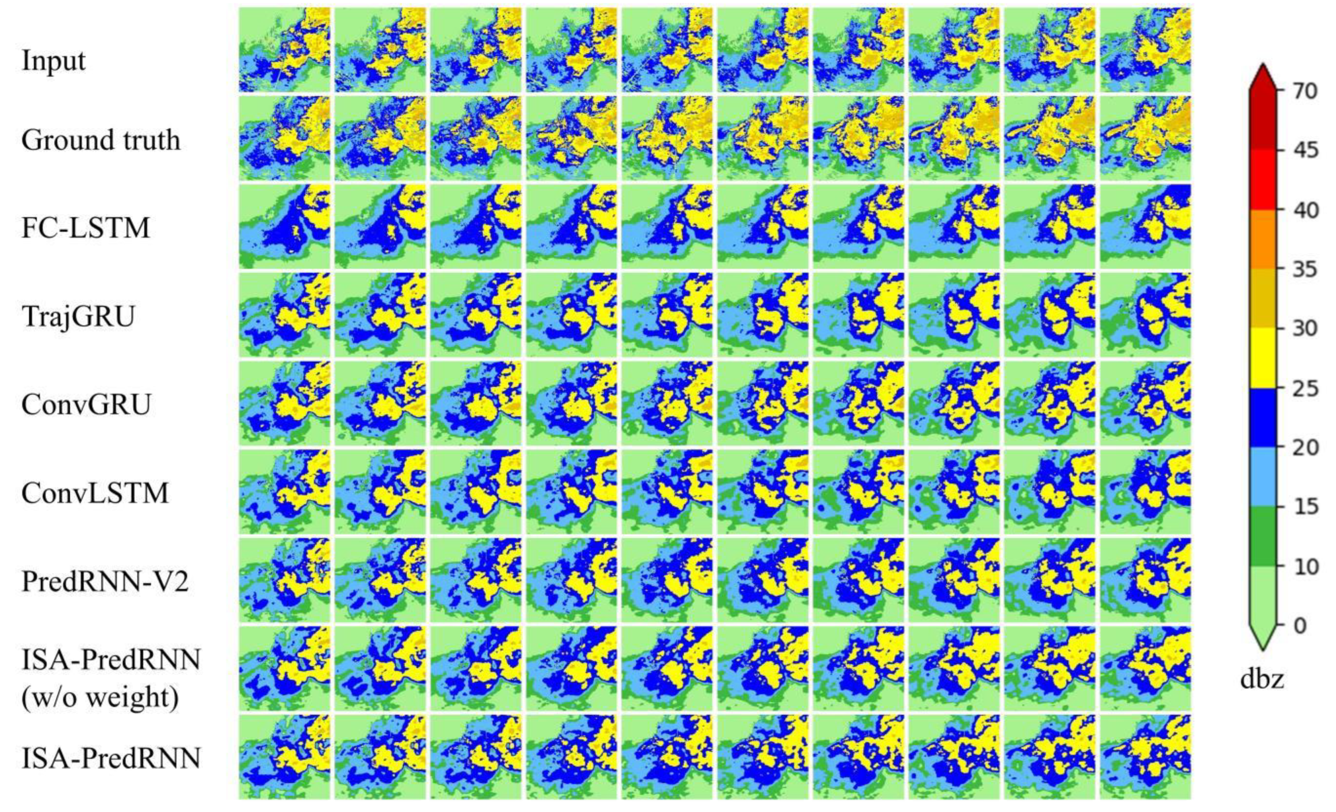
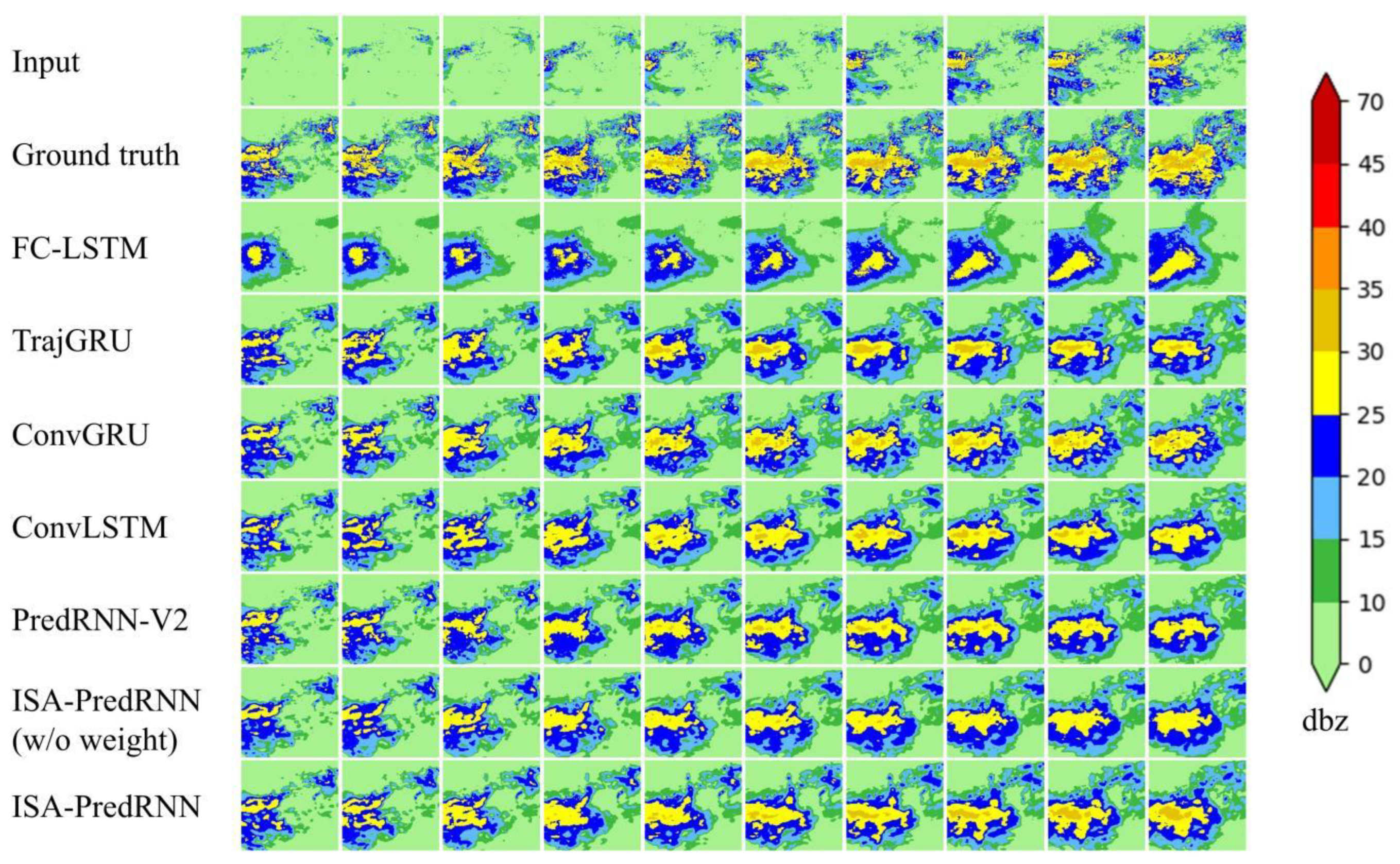
4.3. Analysis and Evaluation of Experimental Results

To further illustrate the effectiveness of the algorithm proposed in this paper in precipitation forecasting, we analyzed and evaluated the experimental results of the new ISA-PredRNN algorithm with six other algorithms. The four index values of POD, FAR, CSI and HSS for each algorithmic at three levels of 10 dBZ, 20 dBZ and 30 dBZ are shown in Table 1, Table 2 and Table 3, and the best mean square error MSE in the test set obtained by each model is shown in Table 4.
From Table 1, Table 2 and Table 3, it can be seen that the new algorithm ISA-PredRNN proposed in this paper has the best performance on the three indicators of POD, CSI and HSS under different thresholds, which indicates that the new model can forecast short-term precipitation more accurately and is more robust. The new algorithm also performs well on the FAR. Although it was higher than the ISA-PredRNN (without weight loss) and PredRNN-V2, it was lower than the other four models. The main reason is that the ISA-PredRNN (without weight loss) and PredRNN-V2 were not able to capture the extremes of precipitation and learn the differences between different levels of precipitation better. They have low POD and FAR because of these. The low FAR is the result of inadequate learning of the distribution of the data. All metrics of all algorithms become progressively worse as the threshold increases, because the probability and area of storm occurrence are small and the network fails to learn the radar echo information corresponding to the storm from the historical data adequately.
Table 4 shows that the ISA-PredRNN achieves the minimum value of MSE, indicating that the error between the predictions and ground truths of precipitation is smaller. This can illustrate that the ISA-PredRNN has stronger spatiotemporal prediction ability and can obtain more accurate radar echo extrapolation results.
In this paper, ten consecutive radar echo maps from the past were used to predict ten consecutive radar echo maps of the future. In order to understand the performance of the model visually, two cases representing two scenarios that often occur with radar echoes in the field of precipitation prediction were selected from the test set for analysis. The radar echo in the first case was strong, concentrated, and subtly variable, while the second case contained the process of radar echo generation, development and dissipation.
Figure 7 shows the results of the first case. In this case, the radar echo was strong, but it changed little. At the 6th minute, the prediction result of ISA-PredRNN was the closest to the ground truth, the FC-LSTM had the worst prediction and could only predict the outline of the radar echo, and other models could predict the overall aspect of radar echo more accurately. By the 18th minute, the ISA-PredRNN preserved the most details in addition to capturing the contours of the radar echoes and the locations of the strong echo regions, while the FC-LSTM model could only roughly predict the contours of the radar echoes and the locations of the strong echo regions, and the other models preserved more details about the differences in the radar echoes. After that, the prediction results of each model gradually became worse, but the ISA-PredRNN could predict the location of the strong echo region better than other models, and the prediction results of FC-LSTM were more different from the ground truth. Overall, the ISA-PredRNN achieved the best prediction results because the attention mechanism and the weight loss function allowed it to capture the differences in precipitation and the extremes of precipitation in different regions better.
Figure 8 shows the results of the second case. In this case, the radar echo was not as strong as that in the first one but changed greatly. The FC-LSTM had poor prediction throughout, but the rest of the models could predict the radar echo results accurately at the 6th minute, among which the ISA-PredRNN had the richest details, and its prediction results were very close to the real situation. By the 18th minute, although some details were lost in the prediction results of each model, the overall contour and change trend of radar echoes could be approximately predicted, and the location of the strong echo region and the difference in radar echo intensity in different regions could be predicted almost accurately, among which the prediction effect of ISA-PredRNN was still the best. Further on, more details were lost, and the differences of some radar echoes were difficult to distinguish. The echo contours predicted by TrajGRU, ConvGRU and ConvLSTM were somewhat different from the ground truths. However, the PredRNN-V2, ISA-PredRNN (without weight loss) and ISA-PredRNN could predict the general contours of the echoes and the locations of the strong echo regions, and the ISA-PredRNN still retained more details in its prediction results. Overall, the ISA-PredRNN captured the radar echo variation most accurately, and the prediction of the FC-LSTM was the most different from the ground truth. This is because the long-term memory state N t in the ISA-PredRNN allowed it to remember the changing trend of the radar echoes, while the FC-LSTM did not contain convolutional structures, which prevented it from handling the changing position information well.

5. Conclusions and Discussions

In this paper, we propose the ISA-PredRNN model for short-term precipitation forecasting, which is an improved structure based on the PredRNN-V2. The self-attention mechanism in the model makes it possible to better extract the global information from the radar echo map. We introduced the long-term memory state into the network architecture and designed a new set of gating mechanisms. These improvements allow the model to better capture long-term memory information and predict more accurately when radar echo images are highly variable. The loss function with weights allows the model to capture the precipitation extremes better. The model was trained using a combination of reverse scheduled sampling and scheduled sampling, which reduces the gap between the training and inference processes. Experimental results on a two-year radar echo dataset in the Yinchuan area of Ningxia show that the ISA-PredRNN proposed in this paper can achieve better performance than the other six models in the most important metrics, whether the radar echoes are in a scene that is strong but does not change significantly with time, or is in a dynamic process of generation and dissipation.
Although satisfactory experimental results have been obtained, there are still some areas for improvement. Due to the uncertainty of the task and the small area and probability of the storm occurring, ISA-PredRNN captures the extreme precipitation while increasing the FAR. Since the atmosphere is a complex dynamical system and there are many factors affecting precipitation, we will subsequently add a variety of factors such as temperature, wind field and barometric pressure as inputs to the network. We will also combine the deep learning model with the numerical weather prediction to further reduce the FAR and improve the accuracy of short-term precipitation forecasts. In recent years, more satellite products have been used for precipitation forecasting with promising results. In future research, we will combine the respective advantages of radar and satellite for precipitation forecasting using multi-source datasets. The main contribution of this paper is to propose a new model and achieve the accurate prediction of future radar echo maps. However, the accurate translation of radar maps into actual precipitation values is challenging as well. In future work, we will focus more on this aspect.

Author Contributions

Conceptualization, D.W. and L.W.; methodology, D.W.; software, D.W. and W.Z.; validation, D.W. and L.W.; formal analysis, W.Z. and J.H.; investigation, W.Z.; resources, L.W. and X.W.; data curation, W.Z.; writing—original draft preparation, D.W.; writing—review and editing, L.W., T.Z., J.H. and X.W.; visualization, D.W.; supervision, L.W., T.Z., J.H. and X.W.; project administration, L.W., T.Z. and J.H.; funding acquisition, T.Z. and X.W. All authors have read and agreed to the published version of the manuscript.

Funding

This research was funded by the National Natural Science Foundation of China (No. 62162053, No. 62062059, No. 62166032) and Natural Science Foundation of Qinghai Province (No. 2022-ZJ-701), the grant (No. SKL-IOW-2020TC2004-01) from Tsinghua University, Key Research and Development Program Project of Ningxia Hui Autonomous Region (2020BCF01002-02), the Open Project of State Key Laboratory of Plateau Ecology and Agriculture, Qinghai University (No. 2020-ZZ-03). Tao Zhang is supported by the Climate Model Development and Validation (CMDV) Project to Brookhaven National Laboratory under Contract DE-SC0012704 and Brookhaven National Laboratory’s Laboratory Directed Research and Development (LDRD) Project 22065.

Institutional Review Board Statement

Not applicable.

Informed Consent Statement

Not applicable.

Data Availability Statement

The radar echo dataset used in this study is openly available in Zenodo at https://doi.org/10.5281/zenodo.6559265.

Acknowledgments

We thank the Institute of High Performance of Qinghai University for providing the computing resources.

Conflicts of Interest

The authors declare no conflict of interest.

References

  1. Dixon, M.; Wiener, G. TITAN: Thunderstorm identification, tracking, analysis, and nowcasting—A radar-based methodology. J. Atmos. Ocean. Technol. 1993, 10, 785–797. [Google Scholar] [CrossRef]
  2. Liang, Q.; Feng, Y.; Deng, W.; Hu, S.; Huang, Y.; Zeng, Q.; Chen, Z. A composite approach of radar echo extrapolation based on TREC vectors in combination with model-predicted winds. Adv. Atmos. Sci. 2010, 27, 1119–1130. [Google Scholar] [CrossRef]
  3. Zhu, J.; Dai, J. A rain-type adaptive optical flow method and its application in tropical cyclone rainfall nowcasting. Front. Earth Sci. 2021, 16, 248–264. [Google Scholar] [CrossRef]
  4. Yang, X.; Kuang, Q.; Zhang, W.; Zhang, G. A terrain-based weighted random forests method for radar quantitative precipitation estimation. Meteorol. Appl. 2017, 24, 404–414. [Google Scholar] [CrossRef] [Green Version]
  5. Bhuiyan, M.A.E.; Anagnostou, E.N.; Kirstetter, P.-E. A nonparametric statistical technique for modeling overland TMI (2A12) rainfall retrieval error. IEEE Geosci. Remote Sens. Lett. 2017, 14, 1898–1902. [Google Scholar] [CrossRef]
  6. Zhang, L.; Li, X.; Zheng, D.; Zhang, K.; Ma, Q.; Zhao, Y.; Ge, Y. Merging multiple satellite-based precipitation products and gauge observations using a novel double machine learning approach. J. Hydrol. 2021, 594, 125969. [Google Scholar] [CrossRef]
  7. Banadkooki, F.B.; Ehteram, M.; Ahmed, A.N.; Fai, C.M.; Afan, H.A.; Ridwam, W.M.; Sefelnasr, A.; El-Shafie, A. Precipitation forecasting using multilayer neural network and support vector machine optimization based on flow regime algorithm taking into account uncertainties of soft computing models. Sustainability 2019, 11, 6681. [Google Scholar] [CrossRef] [Green Version]
  8. Chiang, Y.-M.; Hao, R.; Quan, S.; Xu, Y.; Gu, Z. Precipitation assimilation from gauge and satellite products by a Bayesian method with Gamma distribution. Int. J. Remote Sens. 2021, 42, 1017–1034. [Google Scholar] [CrossRef]
  9. Kolluru, V.; Kolluru, S.; Wagle, N.; Acharya, T.D. Secondary precipitation estimate merging using machine learning: Development and evaluation over Krishna river basin, India. Remote Sens. 2020, 12, 3013. [Google Scholar] [CrossRef]
  10. Chandriah, K.K.; Naraganahalli, R.V. RNN/LSTM with modified Adam optimizer in deep learning approach for automobile spare parts demand forecasting. Multimed. Tools Appl. 2021, 80, 26145–26159. [Google Scholar] [CrossRef]
  11. Nazarova, A.L.; Yang, L.; Liu, K.; Mishra, A.; Kalia, R.K.; Nomura, K.-i.; Nakano, A.; Vashishta, P.; Rajak, P. Dielectric polymer property prediction using recurrent neural networks with optimizations. J. Chem. Inf. Model. 2021, 61, 2175–2186. [Google Scholar] [CrossRef]
  12. Jaihuni, M.; Basak, J.K.; Khan, F.; Okyere, F.G.; Sihalath, T.; Bhujel, A.; Park, J.; Lee, D.H.; Kim, H.T. A novel recurrent neural network approach in forecasting short term solar irradiance. ISA Trans. 2022, 121, 63–74. [Google Scholar] [CrossRef] [PubMed]
  13. Park, M.K.; Lee, J.M.; Kang, W.H.; Choi, J.M.; Lee, K.H. Predictive model for PV power generation using RNN (LSTM). J. Mech. Sci. Technol. 2021, 35, 795–803. [Google Scholar] [CrossRef]
  14. Cho, K.; Van Merriënboer, B.; Gulcehre, C.; Bahdanau, D.; Bougares, F.; Schwenk, H.; Bengio, Y. Learning phrase representations using RNN encoder-decoder for statistical machine translation. arXiv Prepr. 2014, arXiv:1406.1078. [Google Scholar]
  15. Hochreiter, S.; Schmidhuber, J. Long short-term memory. Neural Comput. 1997, 9, 1735–1780. [Google Scholar] [CrossRef]
  16. Alhudhaif, A.; Polat, K.; Karaman, O. Determination of COVID-19 pneumonia based on generalized convolutional neural network model from chest X-ray images. Expert Syst. Appl. 2021, 180, 115141. [Google Scholar] [CrossRef]
  17. Xie, J.; Chen, S.; Zhang, Y.; Gao, D.; Liu, T. Combining generative adversarial networks and multi-output CNN for motor imagery classification. J. Neural Eng. 2021, 18, 46026. [Google Scholar] [CrossRef] [PubMed]
  18. Marques, S.; Schiavo, F.; Ferreira, C.A.; Pedrosa, J.; Cunha, A.; Campilho, A. A multi-task CNN approach for lung nodule malignancy classification and characterization. Expert Syst. Appl. 2021, 184, 115469. [Google Scholar] [CrossRef]
  19. Kolisnik, B.; Hogan, I.; Zulkernine, F. Condition-CNN: A hierarchical multi-label fashion image classification model. Expert Syst. Appl. 2021, 182, 115195. [Google Scholar] [CrossRef]
  20. LeCun, Y.; Bottou, L.; Bengio, Y.; Haffner, P. Gradient-based learning applied to document recognition. Proc. IEEE 1998, 86, 2278–2324. [Google Scholar] [CrossRef] [Green Version]
  21. Krizhevsky, A.; Sutskever, I.; Hinton, G.E. Imagenet classification with deep convolutional neural networks. Adv. Neural Inf. Process. Syst. 2012, 25, 1097–1105. [Google Scholar] [CrossRef] [Green Version]
  22. Shi, X.; Chen, Z.; Wang, H.; Yeung, D.-Y.; Wong, W.-K.; Woo, W.-c. Convolutional LSTM network: A machine learning approach for precipitation nowcasting. Adv. Neural Inf. Process. Syst. 2015, 28, 802–810. [Google Scholar]
  23. Wang, W.; Mao, W.; Tong, X.; Xu, G. A Novel Recursive Model Based on a Convolutional Long Short-Term Memory Neural Network for Air Pollution Prediction. Remote Sens. 2021, 13, 1284. [Google Scholar] [CrossRef]
  24. Liu, Q.; Zhang, R.; Wang, Y.; Yan, H.; Hong, M. Daily prediction of the arctic sea ice concentration using reanalysis data based on a convolutional lstm network. J. Mar. Sci. Eng. 2021, 9, 330. [Google Scholar] [CrossRef]
  25. Kreuzer, D.; Munz, M.; Schlüter, S. Short-term temperature forecasts using a convolutional neural network—An application to different weather stations in Germany. Mach. Learn. Appl. 2020, 2, 100007. [Google Scholar] [CrossRef]
  26. Shi, X.; Gao, Z.; Lausen, L.; Wang, H.; Yeung, D.-Y.; Wong, W.-k.; Woo, W.-c. Deep learning for precipitation nowcasting: A benchmark and a new model. Adv. Neural Inf. Process. Syst. 2017, 30, 5617–5627. [Google Scholar]
  27. Wang, Y.; Long, M.; Wang, J.; Gao, Z.; Yu, P.S. Predrnn: Recurrent neural networks for predictive learning using spatiotemporal lstms. Adv. Neural Inf. Process. Syst. 2017, 30, 879–888. [Google Scholar]
  28. Wang, Y.; Wu, H.; Zhang, J.; Gao, Z.; Wang, J.; Yu, P.S.; Long, M. PredRNN: A recurrent neural network for spatiotemporal predictive learning. arXiv Prepr. 2021, arXiv:2103.09504. [Google Scholar] [CrossRef] [PubMed]
  29. Xu, Z.; Du, J.; Wang, J.; Jiang, C.; Ren, Y. Satellite image prediction relying on gan and lstm neural networks. In Proceedings of the ICC 2019-2019 IEEE International Conference on Communications (ICC), Shanghai, China, 20–24 May 2019; pp. 1–6. [Google Scholar]
  30. Singh, S.; Sarkar, S.; Mitra, P. A deep learning based approach with adversarial regularization for Doppler weather radar ECHO prediction. In Proceedings of the 2017 IEEE International Geoscience and Remote Sensing Symposium (IGARSS), Fort Worth, TX, USA, 23–28 July 2017; pp. 5205–5208. [Google Scholar]
  31. Khan, Z.N.; Ahmad, J. Attention induced multi-head convolutional neural network for human activity recognition. Appl. Soft Comput. 2021, 110, 107671. [Google Scholar] [CrossRef]
  32. Wang, L.; He, Z.; Meng, B.; Liu, K.; Dou, Q.; Yang, X. Two-pathway attention network for real-time facial expression recognition. J. Real-Time Image Process. 2021, 18, 1173–1182. [Google Scholar] [CrossRef]
  33. Li, C.; Zhang, J.; Yao, J. Streamer action recognition in live video with spatial-temporal attention and deep dictionary learning. Neurocomputing 2021, 453, 383–392. [Google Scholar] [CrossRef]
  34. Kim, J.; Li, G.; Yun, I.; Jung, C.; Kim, J. Weakly-supervised temporal attention 3D network for human action recognition. Pattern Recognit. 2021, 119, 108068. [Google Scholar] [CrossRef]
  35. Zhao, Z.; Liu, Q.; Wang, S. Learning deep global multi-scale and local attention features for facial expression recognition in the wild. IEEE Trans. Image Process. 2021, 30, 6544–6556. [Google Scholar] [CrossRef] [PubMed]
  36. Tang, M.; Li, Y.; Yao, W.; Hou, L.; Sun, Q.; Chen, J. A strip steel surface defect detection method based on attention mechanism and multi-scale maxpooling. Meas. Sci. Technol. 2021, 32, 115401. [Google Scholar] [CrossRef]
  37. Cui, X.; Wang, Q.; Dai, J.; Xue, Y.; Duan, Y. Intelligent crack detection based on attention mechanism in convolution neural network. Adv. Struct. Eng. 2021, 24, 1859–1868. [Google Scholar] [CrossRef]
  38. Zhao, H.; Yang, D.; Yu, J. 3D target detection using dual domain attention and SIFT operator in indoor scenes. Vis. Comput. 2021, 38, 3765–3774. [Google Scholar] [CrossRef]
  39. Cao, Z.; Yang, H.; Zhao, J.; Guo, S.; Li, L. Attention fusion for one-stage multispectral pedestrian detection. Sensors 2021, 21, 4184. [Google Scholar] [CrossRef] [PubMed]
  40. Yang, B.; Wang, L.; Wong, D.F.; Shi, S.; Tu, Z. Context-aware self-attention networks for natural language processing. Neurocomputing 2021, 458, 157–169. [Google Scholar] [CrossRef]
  41. Zhang, Y.; Wang, J.; Zhang, X. Learning sentiment sentence representation with multiview attention model. Inf. Sci. 2021, 571, 459–474. [Google Scholar] [CrossRef]
  42. Lin, T.; Li, Q.; Geng, Y.-A.; Jiang, L.; Xu, L.; Zheng, D.; Yao, W.; Lyu, W.; Zhang, Y. Attention-based dual-source spatiotemporal neural network for lightning forecast. IEEE Access 2019, 7, 158296–158307. [Google Scholar] [CrossRef]
  43. Yan, Q.; Ji, F.; Miao, K.; Wu, Q.; Xia, Y.; Li, T. Convolutional residual-attention: A deep learning approach for precipitation nowcasting. Adv. Meteorol. 2020, 2020, 4812. [Google Scholar] [CrossRef]
  44. Sønderby, C.K.; Espeholt, L.; Heek, J.; Dehghani, M.; Oliver, A.; Salimans, T.; Agrawal, S.; Hickey, J.; Kalchbrenner, N. Metnet: A neural weather model for precipitation forecasting. arXiv Prepr. 2020, arXiv:2003.12140. [Google Scholar]
  45. Emerton, R.E.; Stephens, E.M.; Pappenberger, F.; Pagano, T.C.; Weerts, A.H.; Wood, A.W.; Salamon, P.; Brown, J.D.; Hjerdt, N.; Donnelly, C. Continental and global scale flood forecasting systems. Wiley Interdiscip. Rev. Water 2016, 3, 391–418. [Google Scholar] [CrossRef] [Green Version]
  46. Voyant, C.; Haurant, P.; Muselli, M.; Paoli, C.; Nivet, M.-L. Time series modeling and large scale global solar radiation forecasting from geostationary satellites data. Sol. Energy 2014, 102, 131–142. [Google Scholar] [CrossRef] [Green Version]
  47. Schuurmans, J.; Bierkens, M.; Pebesma, E.; Uijlenhoet, R. Automatic prediction of high-resolution daily rainfall fields for multiple extents: The potential of operational radar. J. Hydrometeorol. 2007, 8, 1204–1224. [Google Scholar] [CrossRef]
  48. Hänsel, P.; Langel, S.; Schindewolf, M.; Kaiser, A.; Buchholz, A.; Böttcher, F.; Schmidt, J. Prediction of muddy floods using high-resolution radar precipitation forecasts and physically-based erosion modeling in agricultural landscapes. Geosciences 2019, 9, 401. [Google Scholar] [CrossRef]
Figure 1. Location of Ningxia Hui autonomous region and Köppen classification of Yinchuan. Ningxia Hui autonomous region, highlighted in green, is located in the northwest of China. Yinchuan, as the capital of Ningxia, straddles two climate zones: the warm summer Mediterranean climate (CSB) and the cool semi-arid climate (BSK).
Atmosphere 13 01963 g001
Figure 2. Sample comparison before and after denoising. (a) Original radar echo image. There is some noise caused by various factors in the original image. (b) Denoised image. The denoised image does not contain outliers and can be used directly by the model.
Atmosphere 13 01963 g002
Figure 3. (a) The internal structure of the ST-LSTM. ST-LSTM originates from the basic structural unit of ConvLSTM, with the addition of the spatiotemporal memory state M t as its feature. (b) The propagation of the spatiotemporal memory. The blue arrows indicate that the spatiotemporal state M t is propagated in a zigzag pattern throughout the network.
Atmosphere 13 01963 g003
Figure 4. (a) The operation principle of the self-attention mechanism. The three matrices K x , Q x and V x are originated from the input X . We can extract the global key information of the input X by performing the corresponding operations on K x , Q x and V x . (b) The information processing flow of ISA-LSTM. The final hidden state H ^ t l and the current moment memory state N t l are obtained from the previous moment’s memory state N t 1 l and the intermediate hidden state H t l after being processed by the self-attention module and the corresponding gating mechanism.
Atmosphere 13 01963 g004
Figure 5. Internal structure of the new spatiotemporal memory unit ISA-LSTM. The ISA module consists of two parts: the self-attention mechanism and the GRU-like update gate. Except for the ISA module, the rest of the ISA-LSTM is the same as the basic structural unit of the PredRNN-V2.
Atmosphere 13 01963 g005
Figure 6. (a) The overall network architecture of the original PredRNN-v2. The spatiotemporal memory M t spreads in a zigzag pattern throughout the network, which enhances the network’s use of spatiotemporal information. (b) The overall network architecture of ISA-PredRNN. The newly introduced long-term memory state N t is one of the highlights of this network architecture, which allows the model to pay more attention to the long-term dependence than the original PredRNN-v2.
Atmosphere 13 01963 g006
Figure 7. Prediction examples on the radar echo test set, in which the radar echo was strong but changed little. The ten images in the first row represent the radar echo information of the past hour, and the images in the subsequent rows represent the radar echo information of the future hour obtained by different model predictions. The time interval between adjacent images is 6 min.
Atmosphere 13 01963 g007
Figure 8. Prediction examples on the radar echo test set, in which the radar echo was not as strong as that in the first one but changed greatly.
Atmosphere 13 01963 g008
Table 1. Comparison of the experimental results at the level of 10 dBZ.
ModelCSI↑HSS↑POD↑FAR↓
FC-LSTM0.47710.60600.56540.2476
TrajGRU0.63670.74890.73820.1805
ConvGRU0.66260.77070.75980.1637
ConvLSTM0.66250.77100.70570.1524
PredRNN-V20.68790.79100.77340.1404
ISA-PredRNN(w/o weight)0.69280.79510.77900.1391
ISA-PredRNN0.70010.80060.79210.1435
Note. POD, FAR, CSI and HSS for seven models in the threshold range of radar echo intensity greater than 10 dBZ. ‘↑’ means that the score is higher the better while ‘↓’ means that the score is lower the better.
Table 2. Comparison of the experimental results at the level of 20 dBZ.
ModelCSI↑HSS↑POD↑FAR↓
FC-LSTM0.27110.40750.30130.2716
TrajGRU0.49720.64590.56850.2057
ConvGRU0.52430.67110.59200.1807
ConvLSTM0.52800.67480.59130.1705
PredRNN-V20.54750.69160.60890.1588
ISA-PredRNN(w/o weight)0.56590.70790.63030.1546
ISA-PredRNN0.58120.72080.65420.1630
Note. POD, FAR, CSI and HSS for seven models in the threshold range of radar echo intensity greater than 20 dBZ.
Table 3. Comparison of the experimental results at the level of 30 dBZ.
ModelCSI↑HSS↑POD↑FAR↓
FC-LSTM0.04880.09130.05060.4117
TrajGRU0.20180.32730.21950.2922
ConvGRU0.23430.37070.25780.2758
ConvLSTM0.22900.36470.24670.2379
PredRNN-V20.22260.35310.23680.2075
ISA-PredRNN(w/o weight)0.27380.42170.29500.2055
ISA-PredRNN0.30520.46060.33470.2252
Note. POD, FAR, CSI and HSS for seven models in the threshold range of radar echo intensity greater than 30 dBZ.
Table 4. Best mean square error (MSE) of seven models in the test set.
ModelNumber
of Layer
Number
of Kernel
Kernel SizeMSE
FC-LSTM4128-128-128-1285 × 5178.64
TrajGRU4128-128-128-1285 × 5106.22
ConvGRU4128-128-128-1285 × 593.74
ConvLSTM4128-128-128-1285 × 591.95
PredRNN-V24128-128-128-1285 × 583.53
ISA-PredRNN(w/o weight)4128-128-128-1285 × 579.93
ISA-PredRNN4128-128-128-1285 × 578.27
Note. To obtain fair comparison results, the same network architecture was adopted, and all models had the same number of layers, kernels and kernel size.
Publisher’s Note: MDPI stays neutral with regard to jurisdictional claims in published maps and institutional affiliations.

