Trend Analysis of Hydro-Climatological Factors Using a Bayesian Ensemble Algorithm with Reasoning from Dynamic and Static Variables

Abstract

This study examines the variations in groundwater levels from the perspectives of the dynamic layers soil moisture (SM), normalized difference vegetation index (VI), temperature (TE), and rainfall (RA), along with static layers lithology and geomorphology. Using a Bayesian Ensemble Algorithm, the trend changes are examined at 385 sites in Kerala for the years 1996 to 2016 and for the months January, April, August, and November. An inference in terms of area under the probability curve for positive, zero, and negative trend was used to deduce the changes. Positive or negative changes were noticed at 19, 32, 26, and 18 locations, in that order. These well sites will be the subject of additional dynamic and static layer investigation. According to the study, additional similar trends were seen in SM during January and April, in TE during August, and in TE and VI during November. According to the monthly order, the matching percentages were 63.2%, 59.4%, 76.9%, and 66.7%. An innovative index named SMVITERA that uses dynamic layers has been created using the aforementioned variables. The average proportion of groundwater levels that follow index trends is greater. The findings of the study can assist agronomists, hydrologists, environmentalists, and industrialists in decision making for groundwater resources.

1. Introduction

The whole life cycle of flora and fauna is impacted by hydrological and climatological changes. The combined impact is a new field of study known as hydro-climatology. All the elements of the environment are components of the water cycle, which must constantly be in balance. Life on Earth needs water to survive and be sustained, and the largest freshwater source is groundwater. In India, more than 80% of the country’s needs for drinking water and 60% of its agricultural needs are met by groundwater. In the southernmost state of India, Kerala, freshwater resources are reported to be abundant. As Kerala customarily has a well for each house, the number of groundwater extraction wells has continued to grow throughout time [1]. The idea of determining the causes of oscillations in the groundwater table has arisen as a result of water shortages. Aquifers in Kerala have water depths that range from 0 to 40 mbgl. After the monsoon season, the ground water levels in most areas will be less than 5 mbgl, and subsequently, as a result of extraction, they will fall between 5 and 10 mbgl [2].

The groundwater level analysis initiates an immediate decision-making process for sustainable water management [3]. This can be done with both spatial and temporal scales [4]. Various advancements in the study of groundwater levels include groundwater storage [5,6], potential [7], resource development [8], sustainability [9], usage and management [10], trend analysis [11], and impact on agriculture and the economy [12]. The spatial variability helps the authorities understand the risks of using groundwater [13]. The trend analysis helps to identify the long-term decrease or increase in the levels. The majority of the changes seen in hydro-climatological investigations are dynamic and nonlinear. In contrast, most studies have applied linear trend analysis approaches to these data sets. Mann–Kendall tests, which are also non-parametric, are widely used in the trend analysis of the groundwater level in a particular region, plain, or aquifer all over the globe. To summarize, a monotonic increasing or decreasing linear trend is applied to possibly nonlinear data. The studies related to the groundwater level trend analyses performed all over the globe include those conducted in the city of Jinan in China [14], the northwest part of Uzbekistan [15], the Tabriz plain of Iran [16], the Bacchiglione basin of Italy [17], the Yogyakarta–Sleman basin of Indonesia [18], the KwaZulu-Natal province of South Africa [19], and semi-arid Chile [20]. The trend analysis of groundwater levels carried out by researchers for different parts of India include variations in the depth of the groundwater level in the Kaithal district of Haryana state [21] and the Lower Bhavani River basin in Tamil Nadu [22]; quantification of the groundwater level trends of Gujarat [23], Punjab [24], and the semi-arid region of Telangana [25]; and groundwater variability analysis with rainfall of Jharkhand state [26]. Mann–Kendall tests are used not only for trend analysis of groundwater, but also for precipitation analysis [27,28], deposition data [29], and rainfall [30]. Modified versions of the Mann–Kendall trend test have emerged over the years. Kumar et al. [31] used four variations of Mann–Kendall in determining groundwater level trends. Recent studies have also used the innovative trend analysis method that determines the linear trend using the first and second half of the datasets [32,33,34].

In addition, several nonlinear approaches have been devised to overcome the limitations of the earlier linear methods. One such method is a Bayesian Ensemble algorithm called the Bayesian Estimator of Abrupt change, Seasonal change and Trend (BEAST). The primary concept is to segment the data set into seasonal signal, trend signal, and noise. The Mann–Kendall trend has been applied in a number of groundwater trend analyses, while BEAST has been applied only in a handful of studies. BEAST has several advantages over linear trend analysis methods. It forgoes the single best model concept and embraces all competing models based on Bayesian model averaging. It is a flexible tool to determine abrupt changes, cyclic variations, and nonlinear trends, and it explains how likely the detected changes are true. It is applicable to all real-valued time series datasets. These benefits make it the best method to determine the water table fluctuations. The relevant fields that have applied the BEAST method include remote sensing [35], hydrology [36], hydraulic engineering [37], atmospheric sciences [38], and climate sciences [39]. To the best of our knowledge, BEAST has not been applied to groundwater levels with the considered parameters and an index.

On a primary note, the studies so far have compared the groundwater level trends with respect to rainfall [40]. This is because rainfall acts as a natural recharge. However, in a global analysis and when analyzing a whole state as a domain, like Kerala, it is not sufficient to study just rainfall trends. Due to the rapid increase in the population, urbanization, and industrialization, along with many other developmental activities, the groundwater resources are vulnerable to depletion and quality degradation throughout the state of Kerala [41]. The other dynamic parameters under consideration are temperature, soil moisture, and normalized difference vegetation index (NDVI). The temperature is an indicator of climate change and helps to understand the water fluctuation from a climatological perspective [42]. Soil moisture plays a significant role in the hydrological cycle and tends to influence the groundwater recharge [43]. Rajesh et al. [44] used NDVI to deduce groundwater storage. Various indices are used to explain the characteristics of the groundwater level, such as the standard groundwater level index [45] and the standardized depth to water level index [46]. Presently, all the indices have been created using the levels themselves and inferences such as drought [47,48] are deduced. Studies thus far have not tried to create an index using the influential variables, which take in all the importance and contribution. With the complexity in hydraulic changes, this index can be used to determine the underlying groundwater level changes. The coefficients for the index are obtained from the Analytical Hierarchy Process (AHP). It is a commonly used multi-criteria decision-making technique that strengthens the decision-making process by verifying consistencies [49]. The applications include reinforcement of hydropower strategy [50], comparison of judgment scales [51], potential survey of photovoltaic power plants [52], and investigation of lean-green implementation practices [53]. This is first of its kind to implement AHP for creating a dynamic layer index in determining groundwater fluctuations.

The objective of the study is to analyze the Kerala groundwater level trends using BEAST in order to explain these trend changes with respect to the climatological variables of rainfall and temperature, as well as two other dynamic layers, namely soil moisture and the normalized difference vegetation index. Soil moisture is important because the rainfall needs to penetrate through the soil layer to recharge the source, while VI helps to support water retention. Apart from individual analysis, an index named SMVITERA has been developed and investigated. A final explanation is also obtained from the static layers of lithology and geomorphology. The BEAST aggregates the entire better model, and as a result, the computational part is highly mathematical. The applied studies so far have used the outputs from the model to explain trend changes. In this study, we have deduced a percentage of probability with which the trend could be positive, negative, or zero to explain a comparative level of certainty or significance. The manuscript has been arranged into 5 sections. Section 1 is the Introduction, Section 2 explains the Materials and Methods, Section 3 is the Results, Section 4 details the Discussion, and Section 5 is the Conclusions.

2. Materials and Methods

This section explains the datasets and the methodologies used to carry out this study. The datasets include the primary analysis of groundwater levels and the dynamic and static layers analyzed, whereas the methods include the AHP, Mann–Kendall, and BEAST.

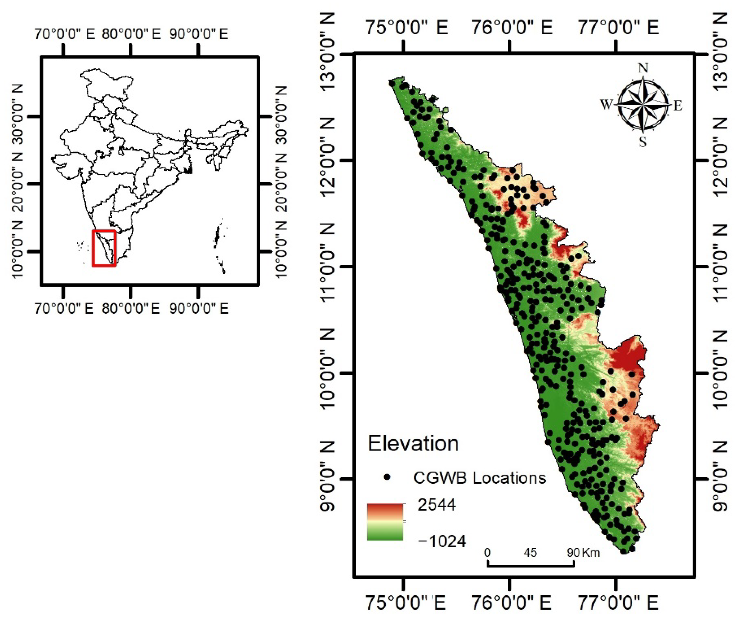
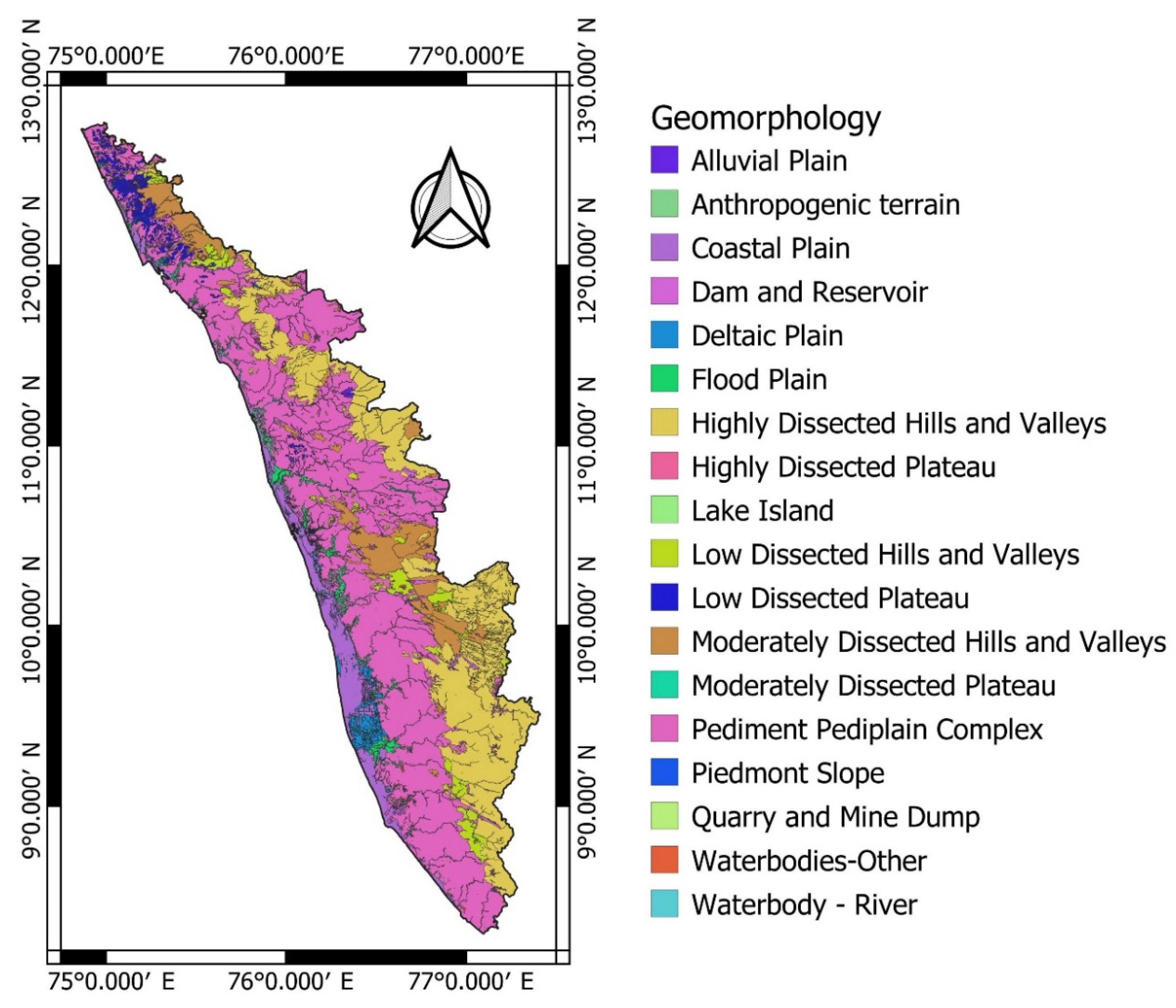
2.1. Study Area and Datasets

The study is conducted in Kerala, which serves as a gateway to the Indian Monsoon. The Arabian Sea to the west, the state of Karnataka to the north, the state of Tamil Nadu to the east, and the Indian Ocean to the south form the borders of Kerala. Kerala, spread over 38,863 km², lies between the latitudes $8^{°} {17}^{\prime }{24}^{″} \mathrm{N}$ to ${12}^{°} {47}^{\prime }{42}^{″} \mathrm{N}$ and between the longitudes ${74}^{°} {51}^{\prime }{46}^{″} \mathrm{E}$ to ${77}^{°} {24}^{\prime }{42}^{″} \mathrm{E}$. Kerala is famed for its natural beauty and backwaters, and the state is home to about 35.33 million people. The state has about 120–140 rainy days, with an average rainfall of about 2923 mm annually and a tropical climate with the seasons Summer (March–May), South–West monsoon (June–September), North–East monsoon (October–November), and Winter (December–February). The mean maximum temperature is $33 ℃$ in March–April and $28.5 ℃$ in July [54]. Kerala has 44 rivers, which annually yield about 70,300 mm³ of water. Even with a copious amount of rainfall, water stress is experienced in different parts of the state during various seasons. The state is split into 14 districts: Kasaragod, Kozhikode, Kannur, Wayanad, Malappuram, Palakkad, Thrissur, Ernakulam, Alappuzha, Idukki, Kottayam, Pathanamthitta, Kollam, and Thiruvananthapuram.

The Central Groundwater Board (CGWB) maintains observation wells around the state to monitor groundwater levels. Meters below ground level (mbgl) are measured four times a year—January, April, August, and November (JAAN)—symbolizing the Winter, Pre-monsoon, Monsoon, and Post-monsoon seasons, respectively. These levels are freely accessible from the India Water Resources Information System (WRIS) (https://indiawris.gov.ins, accessed on 12 January 2022). The wells having at least 90% of the data from 1996 to 2016 during the JAAN months were chosen as suitable research locations, resulting in 385 well locations across the state (Figure 1). The studied well distributions are 41 in Malappuram, 40 in Palakkad, 37 in Thrissur, 34 in Ernakulam, 32 in Thiruvananthapuram, 30 in Kozhikode, 28 in Kollam, 23 in Kannur, 23 in Pathanamthitta, 22 in Alappuzha, 22 in Kottayam, 21 in Wayanad, 20 in Kasaragod, and 12 in Idukki.

2.2. Variable Pre-Processing

The groundwater level characteristics are analyzed with the help of the dynamic layers, namely, Soil Moisture (SM), Normalized Difference Vegetation Index (VI), Temperature (TE), and Rainfall (RA). SMVITERA, an index based on all these layers, has been developed to improvise a combined relationship.

2.2.1. Dynamic Layers

The Global Monthly Soil moisture (in millimeters) from NOAA-NCEP-CPC-GMSM is available as GeoTIFF at the IRI digital library maintained by the International Research Institute of Climate and Society, Columbia Climate School (http://iridl.ldeo.columbia.edu/SOURCES/.NOAA/.NCEP/.CPC/, accessed on 28 January 2022). Soil moisture is assessed by a one-layer hydrologic model [55], which uses observed precipitation and temperature as inputs and computes the soil moisture, evaporation, and runoff [56]. The monthly raster files are downloaded for north latitudes 8° N to 13° N and east longitudes 74° E to 78° E, having a spatial resolution of ${0.5}^{°}\times {0.5}^{°}$ during the years 1996 to 2016 and in the JAAN months. In the Geographic Information System (GIS) environment, the grid point values are extracted and interpolated with the Inverse Distance Weighted (IDW) technique. IDW is calculated using the equation [57]:

$$Z_{\left(S_0\right)}={\displaystyle \sum }_{i=1}^N{\lambda }_i{Z}_{\left(S_i\right)}$$

where N is the number of sampling points, ${\lambda }_i$ is the weightage of each sample point, $S_0$ represents the set of sampling points in the neighborhood of $S_i$, $Z_{\left(S_0\right)}$ is the prediction at $S_0$, and $Z_{\left(S_i\right)}$ is the measured value at $S_i$.

The Normalized Difference Vegetation Index (VI) is an indicator of the greenness of biomes on the Earth’s surface and is essential to monitoring the changes in the ecosystem. The inputs are reprocessed data from SPOT-VEGETATION and PROBA-V missions [58,59,60,61]. The formula used is:

$$NDVI=\frac{RE{F}_{nir}-RE{F}_{red}}{RE{F}_{nir}+RE{F}_{red}}$$

where $RE{F}_{nir}$ and $RE{F}_{red}$ are the spectral reflectance measured in near-infrared and red wavebands. The NetCDF NDVI files are downloaded from Copernicus Global Land Services on a scale of 10 days and 1 km resolution. Three raster images are used and averaged using Cell statistics in GIS to obtain monthly NDVI for the years from 1999 to 2016 and in the JAAN months. Focusing on the Kerala region, it is observed that there are missing values in a few regions. As a result, a model was built in ArcMap that takes these raster layers, converts them into point shapefiles, and then interpolates them using IDW interpolation. Likewise, all the raster layers are created for the considered months.

The climatological data sets on daily rainfall with a spatial resolution of ${0.25}^{°}\times {0.25}^{°}$ [62], and maximum and minimum temperatures of $1^{°}\times 1^{°}$ spatial resolution [63], are downloaded from the India Meteorological Department (IMD) for the years 1996 to 2016 and in the JAAN months. The mean of the maximum and minimum temperatures will be the average temperature. These layers are then linearly interpolated to ${0.25}^{°}\times {0.25}^{°}$. Using the GIS environment, all of these gridded datasets are finally interpolated using the IDW technique and the associated values for the 385 locations, the 21 years (1996 to 2016), and the JAAN months are retrieved.

2.2.2. SMVITERA Index

Each dynamic layer has its own relevance and importance regarding its water holding capacity. Moreover, their positive influence need not always result in an increase in water availability. It is difficult to analyze the variables and their influences separately, and doing so might not yield expected results as well. Here, an approach has been made to create an index based on the above-discussed dynamic layers. The index has been named after combining the layers of Soil Moisture, the normalized difference Vegetation Index, Temperature, and RAinfall to explain the effect in one instance. The formula takes the form:

$$\mathrm{SMIVITERA}=\mathrm{aSM}+\mathrm{bVI}+\mathrm{cTE}+\mathrm{dRA}$$

(1)

Using the Analytical Hierarchical Process (AHP), the coefficients $\mathrm{a}, \mathrm{b}, \mathrm{c}$ and $\mathrm{d}$ are determined as signed normalized weights depending on the influence on water recharge. Depending on how they relate to groundwater recharge, the coefficients are given appropriate signs. The index’s trend analysis aids in pinpointing the combined result and the better one more precisely.

2.2.3. Static Layers

To understand the hydro variability, which assists in determining the land setting under each analyzed place, the static layers of the lithology and geomorphology are examined. The features of a single rock unit found in the Earth’s crust are the subject of the subfield of lithology in Earth sciences. Geomorphology is the study of landforms, including their formation, shapes, and underlying deposits. Bhukosh (https://bhukosh.gsi.gov.in/Bhukosh/Public, accessed on 20 February 2022), a portal and gateway to all geoscientific data of the Geological Survey of India (GSI), is where the lithology and geomorphology of the state of Kerala are found.

2.3. Methods

2.3.1. Analytical Hierarchical Process (AHP)

The Analytical Hierarchical Process (AHP) [64] is applied to obtain the index coefficients, which form a Pairwise Comparison Matrix (PCM). The PCM matrix must be normalized by dividing with the column sum. The weight vector is the average of the total, and then multiplying it by 100 gives the normalized weightage of each variable layer. The consistency of the PCM is found with the help of the Principal Eigenvalue $({\lambda }_{max})$, Consistency Index (CI), and Consistency Ratio (CR). Multiply PCM by the Weight vector (W) to obtain the product matrix (M). Now, divide each of the cells in M by the row value of W to get the Consistency Vector Matrix (CVM), whose average is the Principal Eigenvalue. The Consistency Index is obtained using the equation:

$$CI=\frac{{\lambda }_{max}-n}{n-1}$$

(2)

The Consistency Ratio (CR) is calculated using the equation:

$$CR=\frac{CI}{RI}$$

(3)

where RI denotes the consistency indices for randomly produced reciprocal matrices [65]. The inconsistency is acceptable if CR is less than or equal to 0.1.

2.3.2. Mann–Kendall Trend Test

The Mann–Kendall [66,67] test is a non-parametric test to identify trends, in which all data is compared to all subsequent data. The null hypothesis states that there is no trend and the alternate hypothesis states that there exists an increasing or decreasing trend in the time series. Let $x_1,x_2,x_3,\dots ,x_n$ be a time series of length n. The Mann–Kendall test Statistic S is calculated using,

$$S={\displaystyle \sum }_{k=1}^{n-1}{\displaystyle \sum }_{j=k+1}^{n}sign\left(x_j-x_k\right)$$

where,

$$sign\left(x_j-x_k\right)=\left\{\begin{array}{c} 1 if x_j-x_k>0\\ 0 if x_j-x_k=0\\ -1 if x_j-x_k<0\end{array}\right\}$$

The statistic is normally distributed with mean and variance $E\left(S\right)=0$ and $V\left(S\right)=\frac{1}{18}\left[n\left(n-1\right)\left(2n-5\right)-{\displaystyle \sum }_{p=1}^g{t}_p\left(t_p-1\right)\left(2t_p+5\right)\right]$, where g is the number of tied groups and $t_p$ is the number of data points in the p th group. If there are no tied groups, the variance becomes,

$$V\left(S\right)=\frac{n\left(n-1\right)\left(2n-5\right)}{18}$$

The normalized test statistic Z in the Mann–Kendall test is,

$$Z=\left\{\begin{array}{c}\frac{S-1}{{\left[VAR\left(S\right)\right]}^{\frac{1}{2}}} if S>0\\ 0 if S=0\\ \frac{S+1}{{\left[VAR\left(S\right)\right]}^{\frac{1}{2}}} if S<0\end{array}\right\}$$

Considering a significance level $\alpha$, the null hypothesis is rejected if the absolute value of Z is greater than the table value of $Z_{1-\frac{\alpha }{2}}$. Once the null hypothesis is rejected, the time series exhibits a rise or fall.

The magnitude of the trends is obtained using the Theil–Sens approach [68,69,70], where the slope $\beta$ is given by, $\beta =median\left[\frac{x_j-x_i}{j-i}\right]$, for all $i<j$.

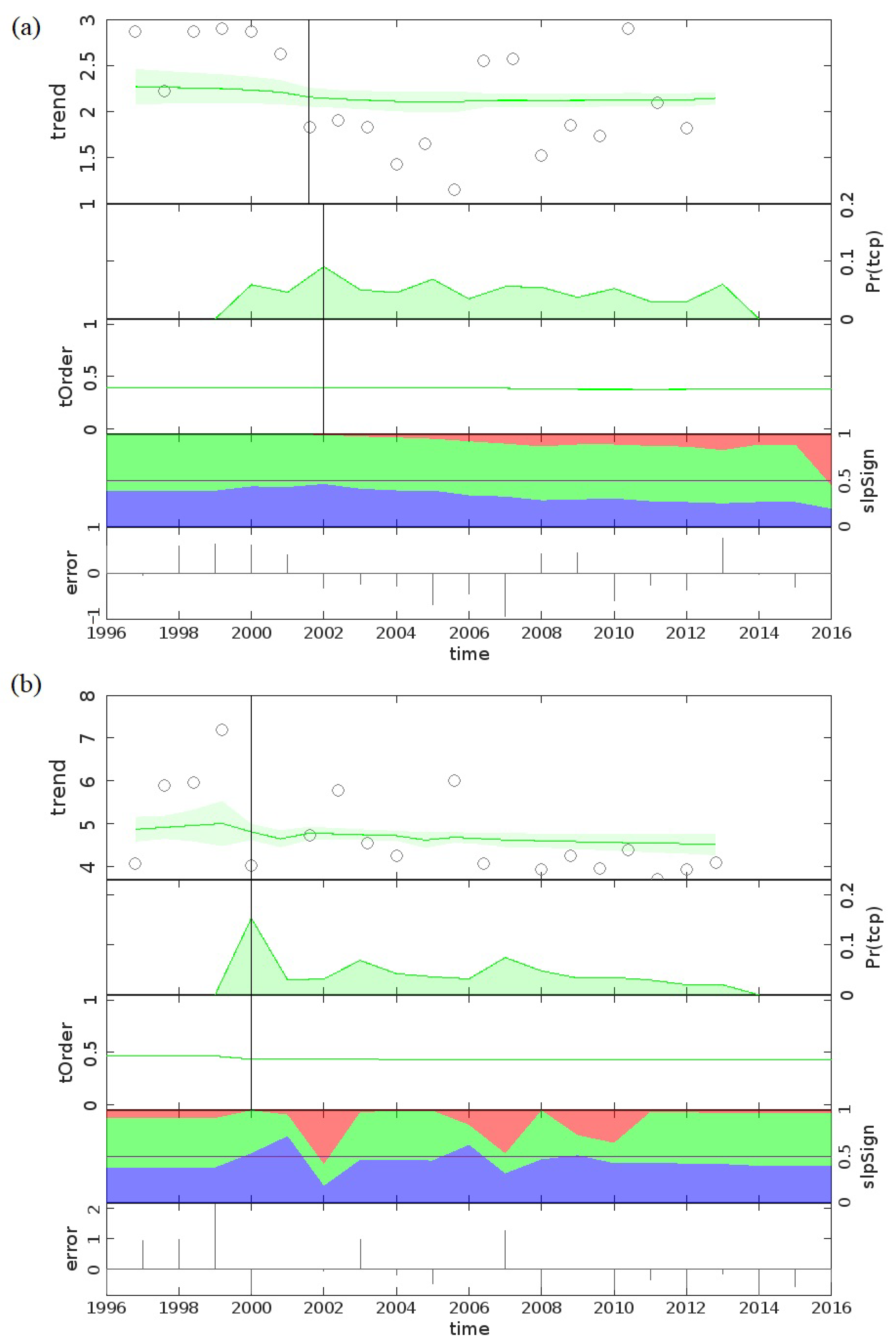
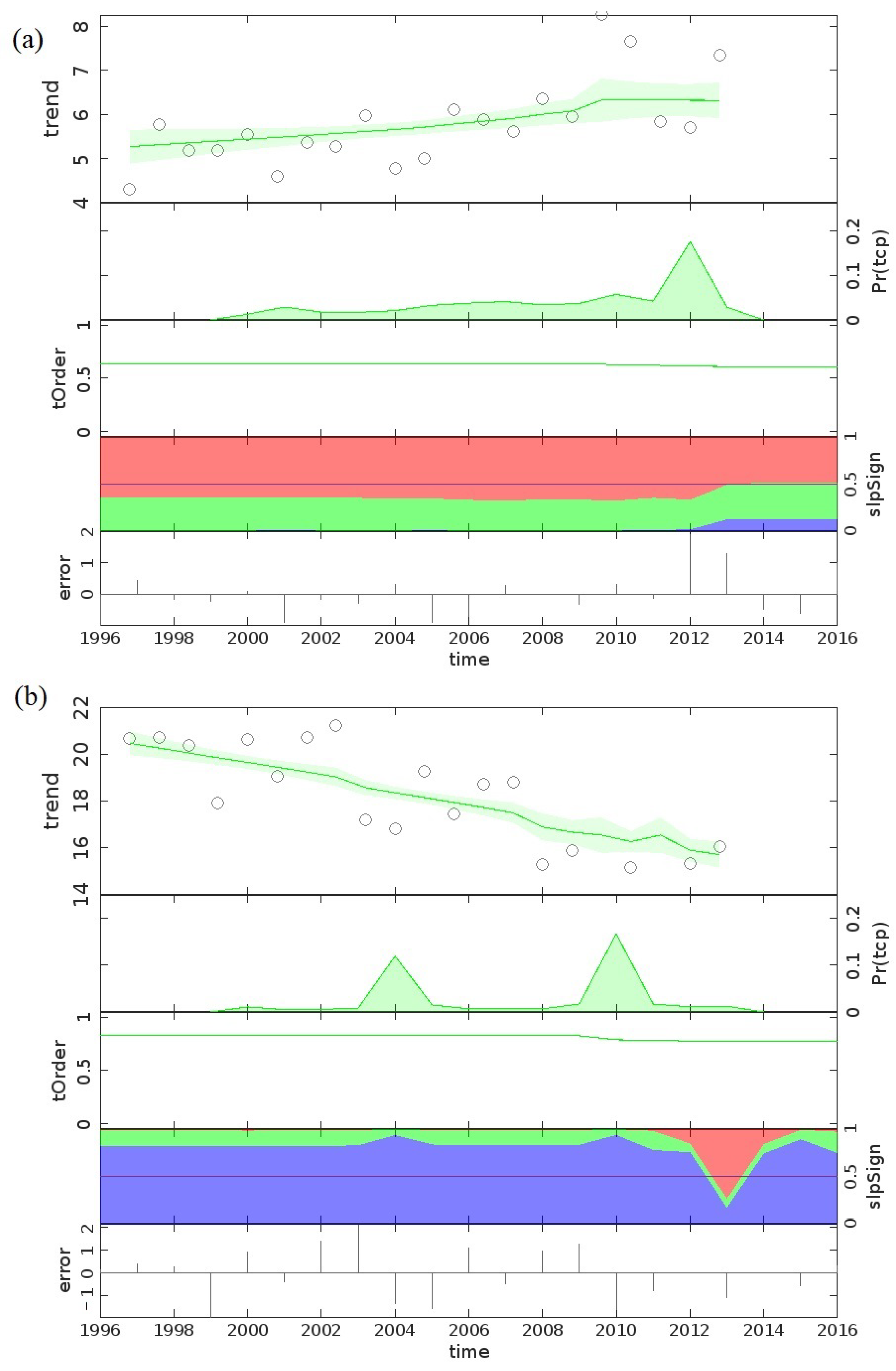
2.3.3. Bayesian Estimator of Abrupt Change, Seasonal Change, and Trend (BEAST)

BEAST is the Bayesian Ensemble Algorithm used to analyze the time series and the change points [71]. The method was initially developed to study satellite time series data and can be applied to any time series that satisfies the assumptions [72]. The model presupposes that a time series can be divided into four components: the seasonal component modeled using a harmonic function, a background component modeled using a piecewise linear regression function, a certain number of possible change points for both of the components, and a certain amount of random noise. The search is for a relationship between the n points of time t and the corresponding data y, combined as time series $D=\left\{y_i,t_i\right\}$ for $i=1,2,\dots ,n$ via a statistical decomposition model $\widehat{y}\left(t\right)=f\left(t\right)$. The model treats the time series $y_i=y\left(t_i\right)$ as a composite of the seasonal S(.) and trend T(.) components, abrupt changes, and the noise, formulated as follows:

$$y_i=S\left(t_i,{\mathsf{\Theta }}_S\right)+T\left(t_i,{\mathsf{\Theta }}_T\right)+{\epsilon }_i$$

(4)

$S(.)$ and $T(.)$ represent the seasonal and trend signals. The noise captures the data that is not explained by these signals ${\epsilon }_i$, which is assumed to follow Gaussian with a magnitude of $\sigma$. The general linear models are adopted to parameterize signals $S(.)$ and $T(.)$ [73,74]. The abrupt changes in the signals are implicitly encrypted in the parameters ${\mathsf{\Theta }}_S$ and ${\mathsf{\Theta }}_T$, respectively.

A piecewise harmonic model is used to approximate the seasonal signal $S\left(t\right)$ with respect to p knots. These p knots divide the time series with starting time ${\xi }_0=t_0$ and ending time ${\xi }_{p+1}=t_n$ into $p+1$ intervals, such as $\left[{\xi }_0,{\xi }_1\right]$, $\left[{\xi }_1,{\xi }_2\right]$,…, $\left[{\xi }_p,{\xi }_{p+1}\right]$. For each of the $p+1$ intervals, denoted by $\left[{\xi }_k,{\xi }_{k+1}\right]$, for $k=0,\dots ,p$, the model takes the form:

$$S\left(t\right)={{\displaystyle \sum }}_{l=1}^{L_k}\left[a_{k,l}sin\left(\frac{2\pi lt}{P}\right)+b_{k,l}cos\left(\frac{2\pi lt}{P}\right)\right], \mathrm{for} {\xi }_k\le t\le {\xi }_{k+1}, k=0,\dots ,p.$$

where P is the period of the seasonal signal, $L_k$ is the harmonic order for the k-th segment, $a_{k,l}$ is the parameter for the sine function, and $b_{k,l}$ is the parameter for the cosine function. The seasonal harmonic curve is specified by the following set of parameters:

$${\mathsf{\Theta }}_S=\left\{p\right\}{\displaystyle \cup }{\left\{{\xi }_k\right\}}_{k=1,\dots ,p}{\displaystyle \cup }{\left\{L_k\right\}}_{k=0,\dots ,p}{\displaystyle \cup }{\left\{a_{k,l},b_{k,l}\right\}}_{k=0,\dots ,p;l=1,\dots ,L_k}$$

A piecewise linear function is used to model the trend signal $T\left(t\right)$ with respect to m knots. These m knots divide the time series with starting time ${\tau }_0=t_0$ and ending time ${\tau }_{m+1}=t_n$ into $m+1$ intervals, such as $\left[{\tau }_0,{\tau }_1\right]$, $\left[{\tau }_1,{\tau }_2\right]$,…, $\left[{\tau }_m,{\tau }_{m+1}\right]$. The trend changepoints denoted by ${\tau }_j$ need not be same as the seasonal changepoint ${\xi }_k$. For each of the $m+1$ intervals, denoted by $\left[{\tau }_j,{\tau }_{j+1}\right]$, for $j=0,\dots ,m$, the model is a line segment of the form:

$$T\left(t\right)=a_j+b_{j}t, \mathrm{for} {\tau }_j\le t\le {\tau }_{j+1}, j=0,\dots ,m.$$

where $a_j$ and $b_j$ are the coefficients. The linear trend curve is specified by the following set of parameters:

$${\mathsf{\Theta }}_T=\left\{m\right\}{\displaystyle \cup }{\left\{{\tau }_j\right\}}_{j=1,\dots ,m}{\displaystyle \cup }{\left\{a_j,b_j\right\}}_{j=0,\dots ,m}$$

The parameters ${\mathsf{\Theta }}_T$ and ${\mathsf{\Theta }}_S$ are reclassified into two groups, M and ${\beta }_M$. The group M refers to the model structure that includes the number and timings of the seasonal and trend changepoints and the seasonal harmonic order.

$$M=\left\{m\right\}{\displaystyle \cup }{\left\{{\tau }_j\right\}}_{j=1,\dots ,m}{\displaystyle \cup }\left\{p\right\}{\displaystyle \cup }{\left\{{\xi }_k\right\}}_{k=1,\dots ,p}{\displaystyle \cup }{\left\{L_k\right\}}_{k=0,\dots ,p}$$

The group ${\beta }_M$ comprises the segment specific coefficient parameters and is used to determine the exact shapes of the seasonal and trend curves.

$${\beta }_M={\left\{a_j,b_j\right\}}_{j=0,\dots ,m}{\displaystyle \cup }{\left\{a_{k,l},b_{k,l}\right\}}_{k=0,\dots ,p;l=1,\dots ,L_k}$$

Thus, Equation (4) becomes the following:

$$y\left(t_i\right)=x_M\left(t_i\right){\beta }_M+{\epsilon }_i$$

(5)

Here, $x_M\left(t_i\right)$ and ${\beta }_M$ are the dependent variables and associated coefficients.

In Bayesian modeling, for the time series $D=\left\{y_i,t_i\right\}$ for $i=1,2,\dots ,n$, the goal is to find the posterior probability distribution $p\left({\beta }_M,{\sigma }^2,M|D\right)$. Using Baye’s theorem, the posterior is the product of the likelihood and a prior model:

$$p\left({\beta }_M,{\sigma }^2,M|D\right)\propto p\left(D|{\beta }_M,{\sigma }^2,M\right)\pi \left({\beta }_M,{\sigma }^2,M\right)$$

(6)

The likelihood being Gaussian is $p\left(D|{\beta }_M,{\sigma }^2,M\right)={\displaystyle \prod }_{i=1}^{n}N\left(y_i;x_M\left(t_i\right){\beta }_M,{\sigma }^2\right)$ and the prior distribution is $\pi \left({\beta }_M,{\sigma }^2,M\right)=\pi \left({\beta }_M,{\sigma }^2|M\right)\pi \left(M\right)$. Firstly, for $\pi \left({\beta }_M,{\sigma }^2|M\right)$, a normal-inverse Gamma distribution is considered and an extra vague dispersion hyper parameter $\nu$ is incorporated to reflect our vague knowledge of ${\beta }_M$. Secondly, for the prior $\pi \left(M\right)$, the number of changepoints are assumed to be non-negative numbers, which is equally probably a prior. Thus, the posterior model Equation (6) becomes:

$$p\left({\beta }_M,{\sigma }^2,\nu ,M|D\right)\propto {\displaystyle \prod }_{i=1}^{n}N\left(y_i;x_M\left(t_i\right){\beta }_M,{\sigma }^2\right)·{\pi }_{\beta }\left({\beta }_M,{\sigma }^2,\nu |M\right)·\pi \left(M\right)$$

The posterior distribution $p\left({\beta }_M,{\sigma }^2,\nu ,M|D\right)$ encodes all the essential information for understanding the ecosystem dynamics. As this is analytically intractable, Markov Chain Monte Carlo (MCMC) sampling is used to generate a realization of random samples for the posterior inference. A hybrid sampler that embeds a reverse jump (RJ) MCMC sampling into a Gibbs sampling framework is used. More details about the RJ-MCMC can be found in Zhao et al. [75].

2.4. Challenges and Betterness

The Mann–Kendall and Bayesian Ensemble Algorithm are assessed through various circumstances and conditions, and the following inferences are obtained:

• Mann–Kendall is a linear, nonparametric trend test often applicable to a monotonic moving dataset. As the real datasets on hydro climatological factors exhibit vibrant and non-cyclic changes, fitting a linear trend is not apt. The Bayesian algorithm overcomes this challenge by finding piecewise linearly fitted trends.
• The Mann–Kendall trend test fits a single trend line to the datasets. The interpretation of time series solely depends on the models being utilized and finding the optimal models is never easy. BEAST offers the single best model approach and adopts the concept of embracing all the models using the Bayesian model averaging scheme, which is always better.
• Sen’s slope technique produces an overall slope for the Mann–Kendall test. BEAST provides the slope at each time series point of the data sets. Additionally, the Bayesian process may be used to determine how likely an event is to occur.
• The data point is removed from computations using the Mann–Kendall test if there are any missing values. Consequently, the trend analysis only considers non-NaN or non-missing variables, while the final fitted trend in BEAST will be continuous even when missing values are provided, eliminating the repercussions of missing values and discontinuity in the outcome.
• Mann–Kendall is highly sensitive to outliers, while the sensitivity is comparatively less for the Bayesian approach. BEAST studies the nature of the whole dataset rather than focusing on the end points.

2.5. Inference and Modulation

An advantage of Mann–Kendall over BEAST is that the significance level can be stated for the increasing or decreasing trend. To solve this, we used the implications from the percentage areas of positive, zero, and negative slope from the output to conclude which is greater. The method varies from traditional trend analysis in that it yields findings that take into account the likelihood of the slope. In other words, it is possible to determine the probability that the slope will be positive, zero, or negative at each time series point.

The BEAST has five major components. The first component is the piecewise linear trend along with the change point detected, the second component is the probability of the trend change point occurrence over the considered time, the third component is the order of the time-varying polynomial needed to approximate the fitted trend, the fourth component is the probabilities of the trend, and the fifth component is the error. Let the probability time series of the positive slope be denoted as $p\left(x\right)$, negative slope be denoted as $n\left(x\right)$, and zero slope be denoted as $z\left(x\right)$, for $i=1,\dots ,N$. The area A under these probabilities is calculated using the trapezoidal method, formulated as:

$$A={{\displaystyle \int }}_a^{b}f\left(x\right)dx\approx \frac{b-a}{2N}{\displaystyle \sum }_{n=1}^N\left(f\left(x_n\right)+f\left(x_{n+1}\right)\right)$$

The percentage area will be $PA=\frac{A}{N-1}\times 100$.

The percentage area under each of the probability curves supplies information regarding the overall slope of the fitted trend. The greater percentage areas are taken into account to explain the nature of trend. These percentages are used instead of the significance level to convey the confidence of getting a particular trend. The piecewise linear trend helps to identify the deflection in slope at each location. Deducing an overall slope sign is explained in relation to the greatest percentage, while the slope is obtained by linearly fitting the time series trend data sets.

3. Results and Discussion

This section deals with the trend results obtained using BEAST over the datasets of groundwater levels, rainfall, temperature, soil moisture, NDVI, and SMVITERA index. The trends of these variables are compared with the groundwater level trends to obtain feasible interpretations about the influences occurring in the context of the considered years. The groundwater level trends are explained using the dynamic layers and the introduced index, as well as the static layers.

3.1. SMVITERA Index Formulation

The index acts as an integrated variable of the studied dynamics. The initial layer weights are assigned using Satty’s scale, on a scale of 1 to 9. The value 1 implies equal significance, 3 indicates moderate relevance, 5 indicates strong importance, 7 indicates extremely strong importance, and 9 indicates extreme importance. The intermediate numbers 2, 4, 6, and 8 correspond to the intermediate effects. The weights are set based on the variable relevance and contribution to the water holding capacity. The vegetation index is assigned weight 8, moisture is assigned 7, rainfall is assigned 4, and temperature is assigned 2. The Pairwise Comparison Matrix (PCM) is shown in

Table 1. Pairwise comparison matrix for the variable layers.

Thematic Layer	Assigned Weight	VI	SM	RA	TE
VI	8	8/8	8/7	8/4	8/2
SM	7	7/8	7/7	7/4	7/2
RA	4	4/8	4/7	4/4	4/2
TE	2	2/8	2/7	2/4	2/2

, and the normalized PCM and the final matrices are shown in

Table 2. Normalized pairwise comparison matrix and the final matrices.

Thematic Layer	VI	SM	RA	TE	Total	Weight Vector (W)	Weightage	Product Matrix	Consistency Vector Matrix (CVM)
VI	8/8	8/7	8/4	8/2	1.52	0.38	38	1.52	3.998
SM	7/8	7/7	7/4	7/2	1.33	0.33	33	1.33	4.006
RA	4/8	4/7	4/4	4/2	0.76	0.19	19	0.76	3.998
TE	2/8	2/7	2/4	2/2	0.38	0.10	10	0.38	4.015

.

It is obtained that the normalized weights are 38 to normalized difference vegetation index, 33 to soil moisture, 19 to rainfall, and 10 to temperature. The Principal Eigenvalue is:

$${\lambda }_{max}=\frac{3.998+4.006+3.998+4.015}{4}=\frac{16.017}{4} =4.00425$$

The Consistency Index for $n=4$ is calculated as follows:

$$CI=\frac{4.00425-4}{4-1}=\frac{0.00425}{3}=0.0014167$$

For $n=4,$ RI is 0.89. The Consistency Ratio (CR) is calculated as:

$$CR=\frac{0.0014167}{0.89}\approx 0.001592$$

Since the obtained CR is much less than the threshold value, the PCM exhibits a high level of consistency.

The variables soil moisture and temperature are inversely proportional to groundwater levels. As a result, these layers are assigned negative signs in calculating the SMIVITERA index for 1999 to 2016.

$$\mathrm{SMIVITERA}=-33\mathrm{SM}+38\mathrm{VI}-10\mathrm{TE}+19\mathrm{RA}$$

3.2. General Characteristics of Variables

The analysis is on 385 well locations over Kerala state during January, April, August, and November. Groundwater levels aid in determining how much freshwater is available for consumption. It also helps in analyzing the past, tracking the present, and forecasting the future. For the years from 1996 to 2016, the average groundwater level was 0.63 to 23.48 mbgl in January, 0.82 to 24.11 mbgl in April, 0.35 to 22.03 mbgl in August, and 0.36 to 22.81 mbgl in November. The depth to water level can be used to calculate inverse water availability. For instance, the depth to water level being 2 mbgl and 5 mbgl indicates that the well with a recorded water level of 2 mbgl contains more water than the well with a water level of 5 mbgl. The variables analyzed to groundwater levels include a combination of dynamic and static layers. The dynamic variables are Soil Moisture (SM), Normalized Difference Vegetation Index (VI), Rainfall (RA), Temperature (TE), and a developed Groundwater Index (SMVITERA) based on the former dynamic layers. Lithology (LI) and geomorphology (GM) are the static factors investigated.

Rainfall and temperature are climatological factors that influence groundwater levels. Rainfall is the natural source of recharge to groundwater, but as the temperatures rises, more water is needed for all living things to consume. However, increased rainfall may not necessarily result in increased recharge since the other variables influence the site. The daily average rainfall for January, April, August, and November are evaluated. The daily rainfall values range from 0 to 0.37 mm during January, 0 to 3.986 mm during April, 0 to 26.753 mm during August, and 0 to 5.66 mm during November. It is observed that the summer or pre-monsoon season receives more average rainfall than the winter season. Temperature ranges are comparably narrower. Temperatures vary from 20.55 to 26.34 °C in January, 23.18 to 29.05 °C in April, 20.52 to 27.43 °C in August, and 20.94 to 26.53 °C in November. Temperature ranges are highest in April due to summer and lowest in January due to winter. The average groundwater levels, rainfall, and temperature for the years from 1996 to 2016 during the JAAN months is shown in Figure 2.

The soil characteristics, such as its moisture content, help to determine the water permeability of the soil. As surface moisture increases, the water condenses on the Earth surface and does not contribute to the underlying groundwater. During the months of January, April, August, and November, it is observed that the soil moisture varies from 98.04 to 148.27 mm, 60.59 to 111.54 mm, 109.78 to 238.78 mm, and 132.33 to 203.89 mm, respectively. Owing to the monsoon, soil moisture levels are highest in August and lowest in April due to the summer season. The normalized difference vegetation index is in the range of 0 to 1. The closer the index is to 1, the greater the content of greenery in the region. The observed ranges are 0.37 to 0.83 in January, 0.29 to 0.8 in April, 0.28 to 0.75 in August, and 0.37 to 0.82 in November. With the help of all these values of dynamic layers, the SMVITERA index is calculated. The obtained index value lies in the range −5097.24 to −3368.55 in January, −3957.95 to −2216.27 in April, −8031.24 to −3426.74 in August, and −6864.86 to −4436.84 in November. The average soil moisture, NDVI, and SMVITERA index during the JAAN months are shown in Figure 3.

Over the state of Kerala, 77 divisions of lithological formations are found (Figure 4). Most of the state is covered by Acid to Intermediate Charnockite and the least by Terri Sand. The lithological formations of the studied 385 locations are of 27 categories: Acid to intermediate charnockite, Biotite gneiss, Clay, Clayey sand, Diorite, Gabbro, Garbiosill gneiss+graphite+kyanite, Garnet gneiss, Garnet biotite gneiss, Garnet sillimanite gneiss+graphite+cordierite, Granite, Granite gneiss, Grey fine sand, Hornblende biotite gneiss, Hornblende biotite syenite, Laterite, Mica Schist, Mylonite, Pyroxene granulite, Quartzite, Sand (active channel as well), Sandstone, Sericite schist, Talc tremolite actinolite, schist, and Terri Sand. A total of 18 geomorphological formations are found in the state of Kerala (Figure 5). Most of the state is covered by Pediment Pediplain Complex and Highly Dissected Hills and Valleys. Over the 385 well locations that have been studied, the formations found are Alluvial plain, Coastal plain, Dam and Reservoir, Deltaic plain, Flood plain, Low dissected plateau, Pediment pediplain complex, Waterbody—river, and also highly, moderately, and low dissected hills and valleys.

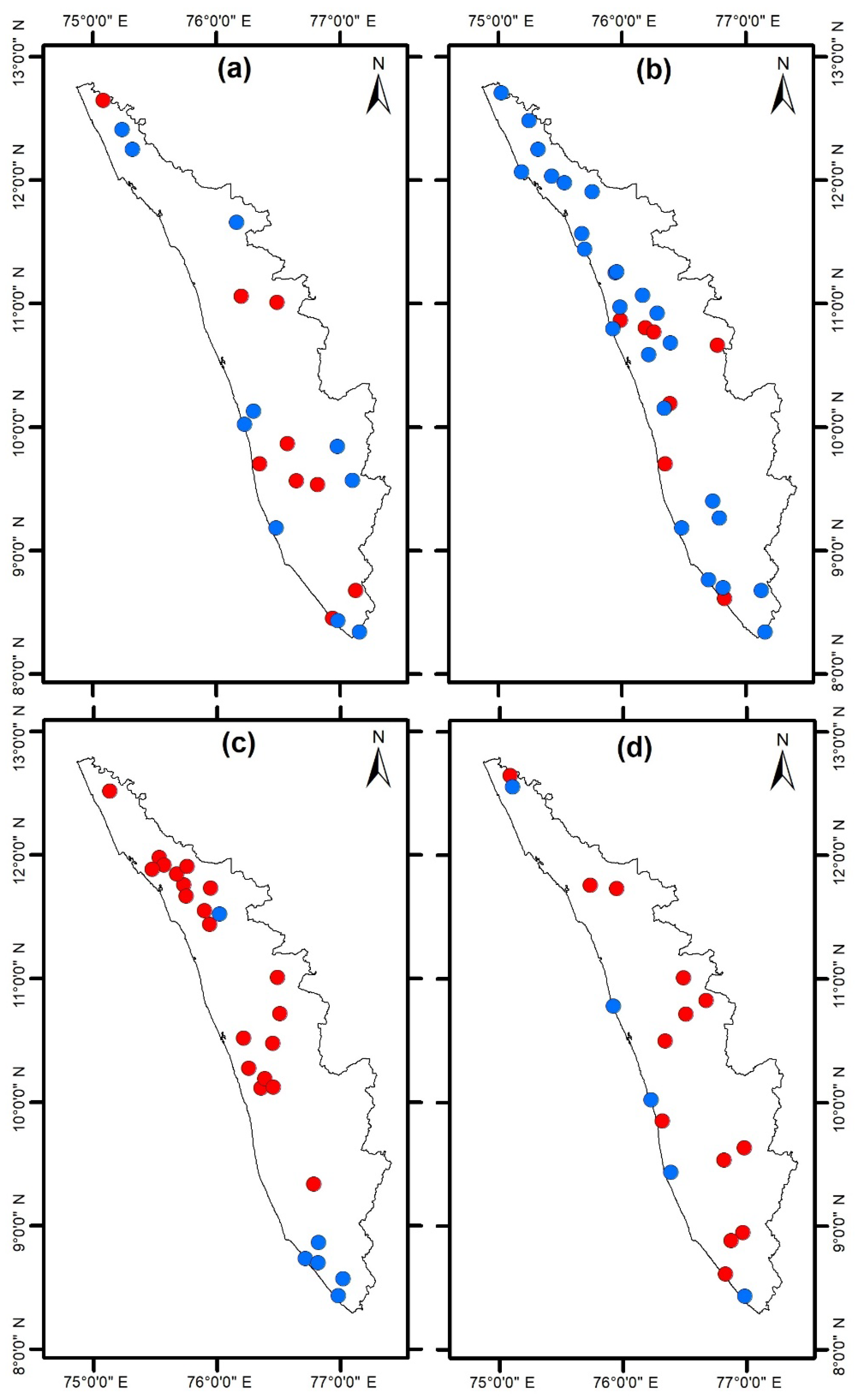
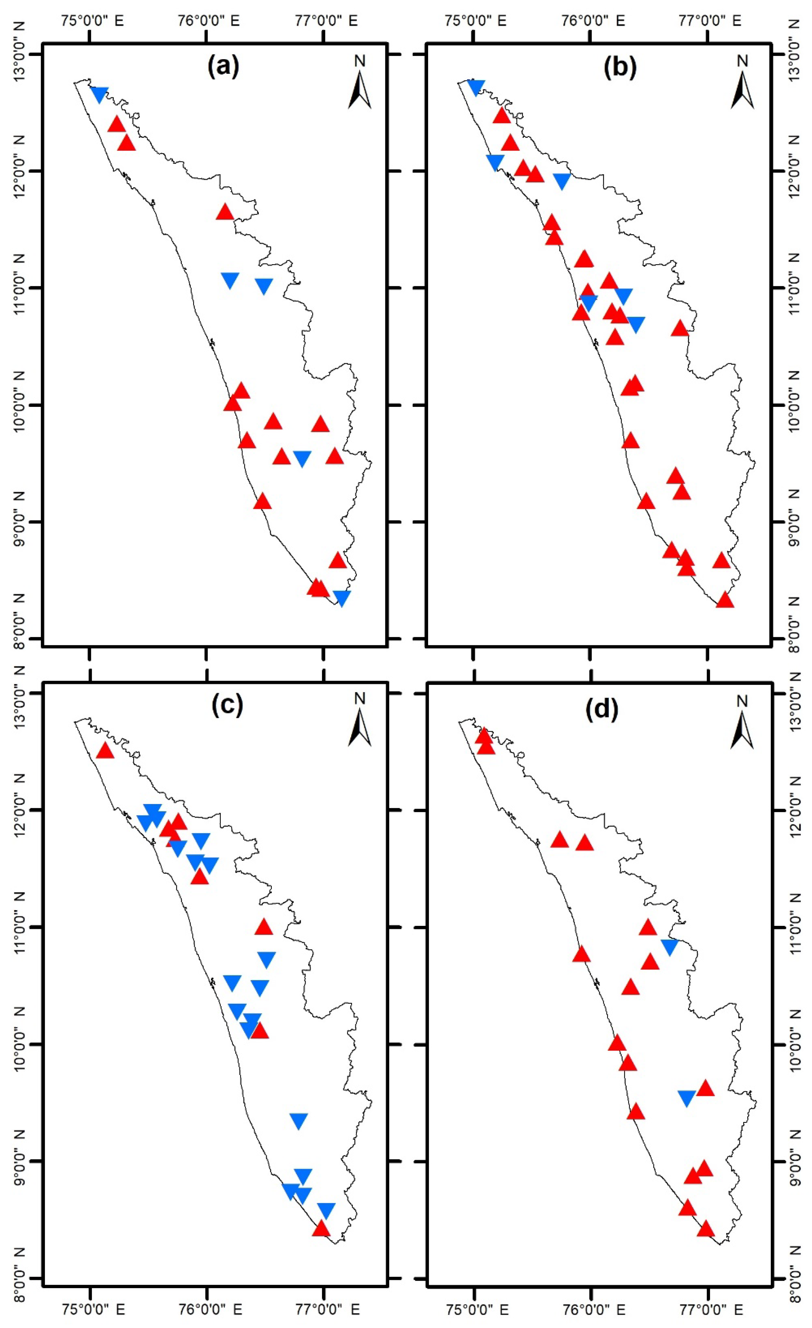
3.3. Groundwater Level Trend Analysis

The BEAST is performed over the 385 sites and individually for the JAAN months. The time series has 21 time points and spans the years 1996 to 2016. The groundwater level dataset is fitted with a piecewise linear trend even in the presence of missing values using BEAST. At each of the 21 time points, the slope of this fitted trend is also determined. The sites having the percentage areas greater in the positive or negative slope are chosen as the locations for further analysis. This positivity or negativity is also verified by linearly modelling the trend data points. Over the studied 385 locations, a combination of probabilities is obtained. During the month of January, the Well number 1 (Konnakuzhi-iii) situated in the Ernakulam district showed the greater probability of groundwater level trend to be zero (Figure 6a). That is, the green area indicating zero slope dominates in the graph. The percentage areas were 7.9% for positive slope, 58.7% for zero slope, and 33.4% for negative slope. The linear modelling showed the slope to be −0.0068, approximately zero, and the negative slope contribution is visible as the second highest percentage as well. Another example is during the month of April on the well number 170 (Kottanadu) situated in Pathanamthitta district, which showed the areas of green and blue approximately to be the same (Figure 6b). This means that there exists an approximately equal probability for the slope to be zero and negative. The percentage areas were obtained as 12.1% for positive slope, 43.3% for zero slope, and 44.6% for negative slope. We are typically interested in the well locations where the probability for negative or positive is the highest over each site. One such example is well location 20 (Pattambi) situated at Palakkad district, which has a greater percentage for positive slope during the month of April (Figure 7a), and well location 32 (Poonkulam) in Thiruvananthapuram district, which has a greater percentage for negative slope during the month of August (Figure 7b). The percentage areas are around 63.9% and 79.9%. The linearly modelled slopes are 0.0634 and −0.246.

In the month of January, 19 locations resulted in comparatively positive or negative slope probability percentage areas. The locations are Poonkulam, Pambadi, Minangadi, Vayyakara, Angadimogar, Rajapuram, Cherthalai, Tachinganedam, Malipuram, Tenkara, Kuvapalli, Kayamkulam, Idukki, Parassala, Maruthamala, Vandiperiyar, Poonthura, Kuttattukulam, and Kottapuram2. The district-wise distribution is four in Thiruvananthapuram; three in Ernakulam; two each in Alappuzha, Idukki, Kasaragod, and Kottayam; and one each in Kannur, Malappuram, Palakkad, and Wayanad. Out of these, 10 locations have negative groundwater level trend, while nine wells have positive groundwater level trend. The areas under the probabilities of positive trend vary from 51.6% to 89.5%, while the area under the probabilities of positive trend varies from 48.6% to 88.7%. The greatest percentage for positive trend is observed in the Tenkara location and the linear model showed the slope to be 0.0622, whereas the greatest percentage for negative trend is observed in the Kottapuram2 location and the slope obtained through linear modeling is −0.0512.

During the month of April, a total of 32 locations had greater percentages for slope to be positive or negative. The well location names are Chamravattom, Pattambi, Quilandy, Mavoor-ii, Mudikode, Vayyakara, Edavai, Thirunavaya, Ramantalai, Irikkur, Kottakkal, Chelakod, Thiruvallur, Cherthalai, Kottanadu, Chengamanad, Kayamkulam, Parassala, Shoranur, Mulankunnathukavu, Angamali1, Bandadka, Manattana, Pukkundu, Paral, Attingal, Palghat, Muligadde, Maruthamala, Mavoor-I, Murukumpuzha (R1), and Pathanamthitta. The district-wise well distribution is two each in Alappuzha, Ernakulam, Kasaragod, Pathanamthitta, and Thrissur; three in Palakkad; four in Kozhikode; and five each in Kannur, Malappuram, and Thiruvananthapuram. Out of these, 7 locations showed positive trend and 25 locations showed negative trends. The area under the probabilities of positive trend varies from 46.1% to 92.9%, while the area under the probabilities of negative trend varies from 42.5% to 81.3%. The greatest percentage for negative trend is observed in the Mavoor-I location and the linear model showed the slope to be 0.0622, whereas the greatest percentage for positive trend is observed in the Thirunavaya location and the slope obtained through linear modeling is −0.0512.

In the month of August, a total of 26 wells showed trend changes. The locations are Kakkayam, Alwaye, Tholanur, Poonkulam, Pudukayam, Irikkur, Aruvikara, Mattanur, Perambra, Trichur, Akkal, Devarkoil, Lakkidi, Tenkara, Vellamunda, Kannavam, Varkala, Muliyar, Angamali1, Manattana, Cherukunnu, Attingal, Puthenchira, Elanthur, Vallom1, and Chakkarakkale. The positive trend locations count to 20 and negative trend locations count to 6. The month of August represents the monsoon season in Kerala, and the results show positive groundwater level trends in most of the well locations. The possible explanation is that the amount of water getting recharged has reduced, or over-exploitation has occurred. The percentages of area obtained lies in the range 48.9% to 83.7% for negative slope and 46.6% to 92.1% for positive slope.

The post monsoon season is indicated by the month of November. Eighteen wells showed positive or negative groundwater level trends over the studied 385 locations. The wells are Ponnani1, Tholanur, Poonkulam, Pudukayam, Arukutti, Angadimogar, Nedumudi (pupalli), Malipuram, Tenkara, Vellamunda, Kuvapalli, Manamangalam, Mavinakatta, Malampuzha, Ailara, Elappara, Murukumpuzha (R1), and Chadayamangalam1. Out of these locations, 5 wells showed negative trend and 13 wells showed positive trend. The percentages of area obtained lies in the range 47.1% to 50.7% for negative slope and 48.6% to 86.1% for positive slope. It is observed that the percentage that indicates a declining trend of depth to water level is less during the month of November.

From the positive trend, the inference is that the depth to groundwater levels is increasing and, as a result, the water availability is decreasing. Thus, a track on positive trend wells provides a balance to the water table. The focus locations 19, 32, 26, and 19 during the respective JAAN months is shown in Figure 8. The red-colored locations denote positive trend and the blue-colored location denote negative trend.

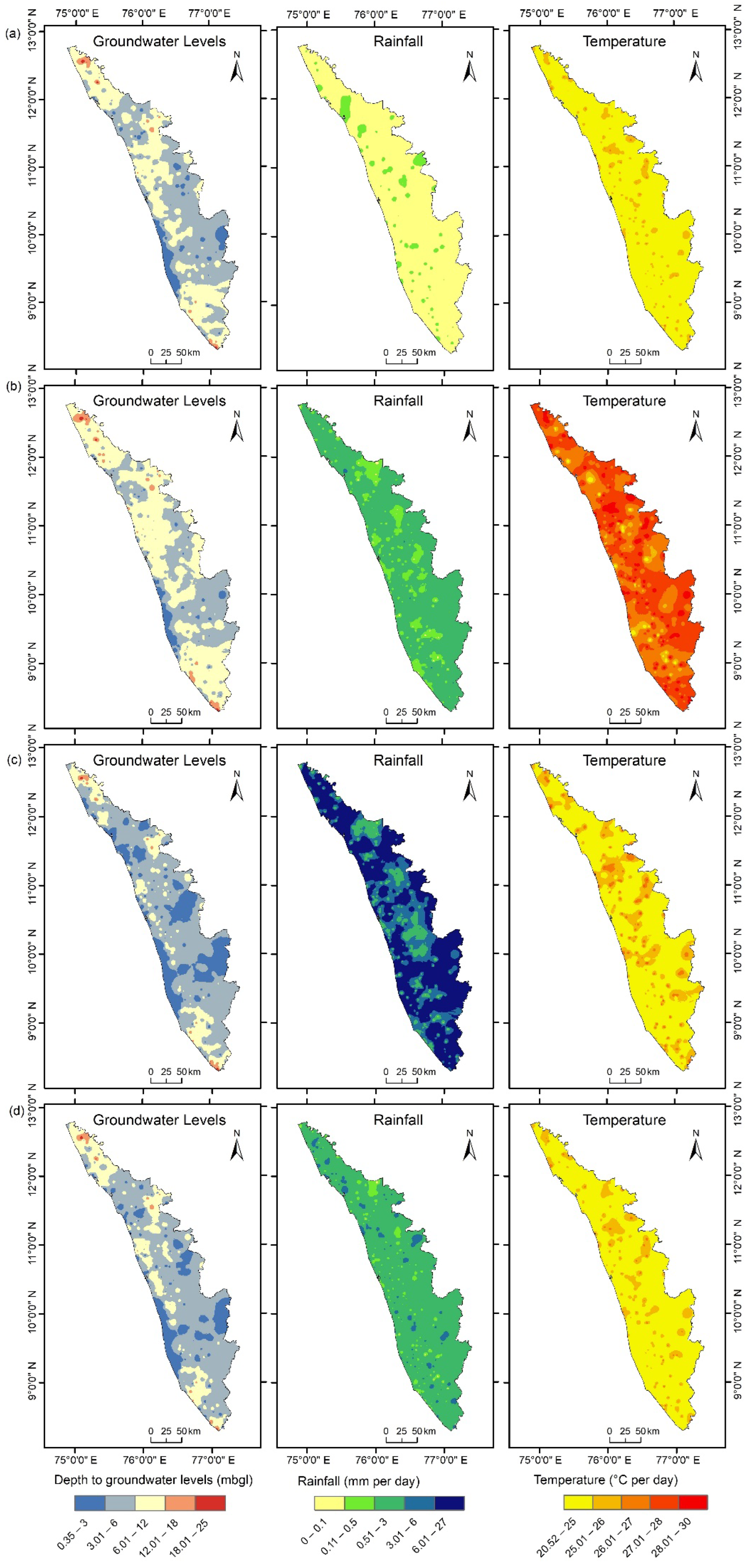
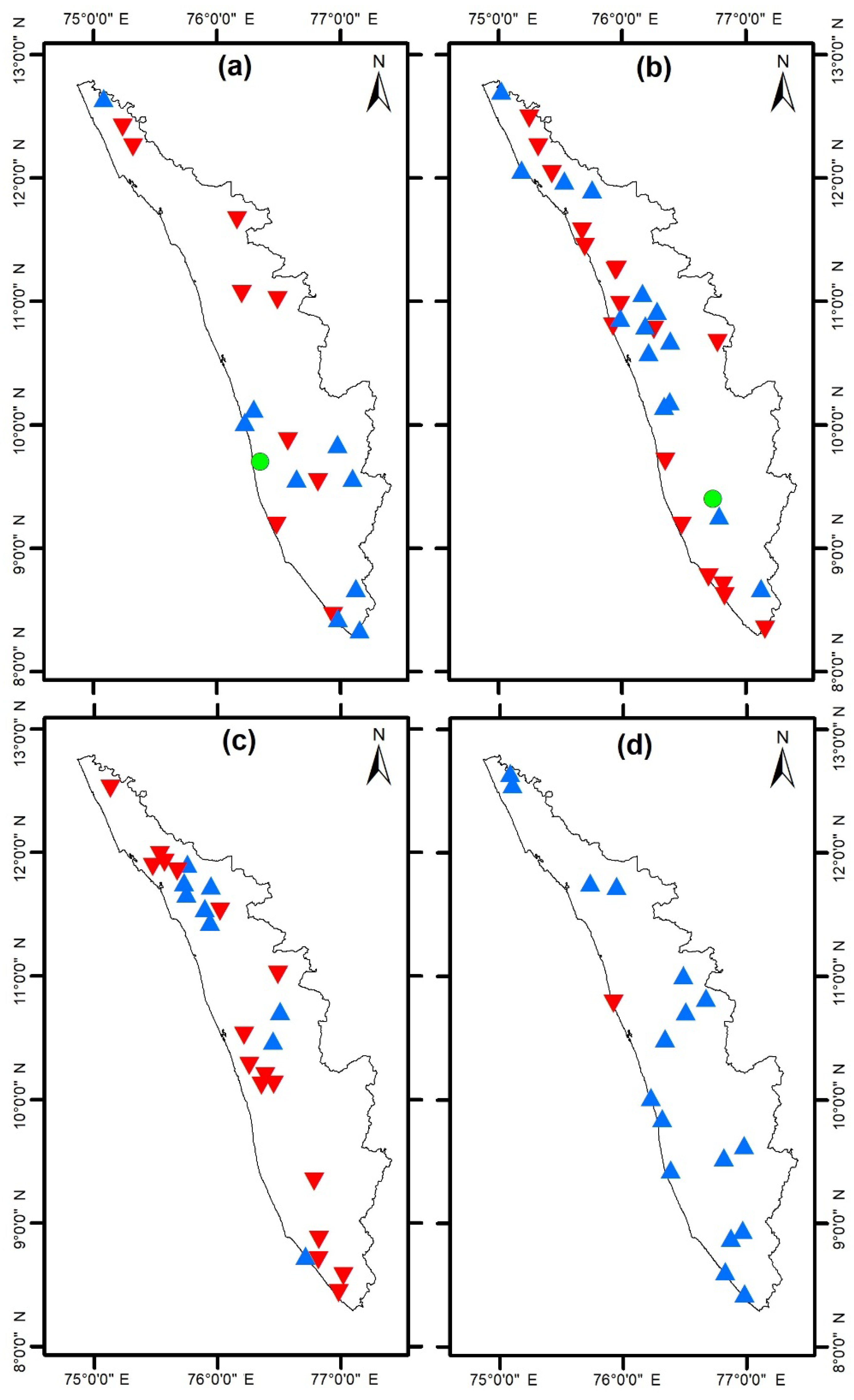
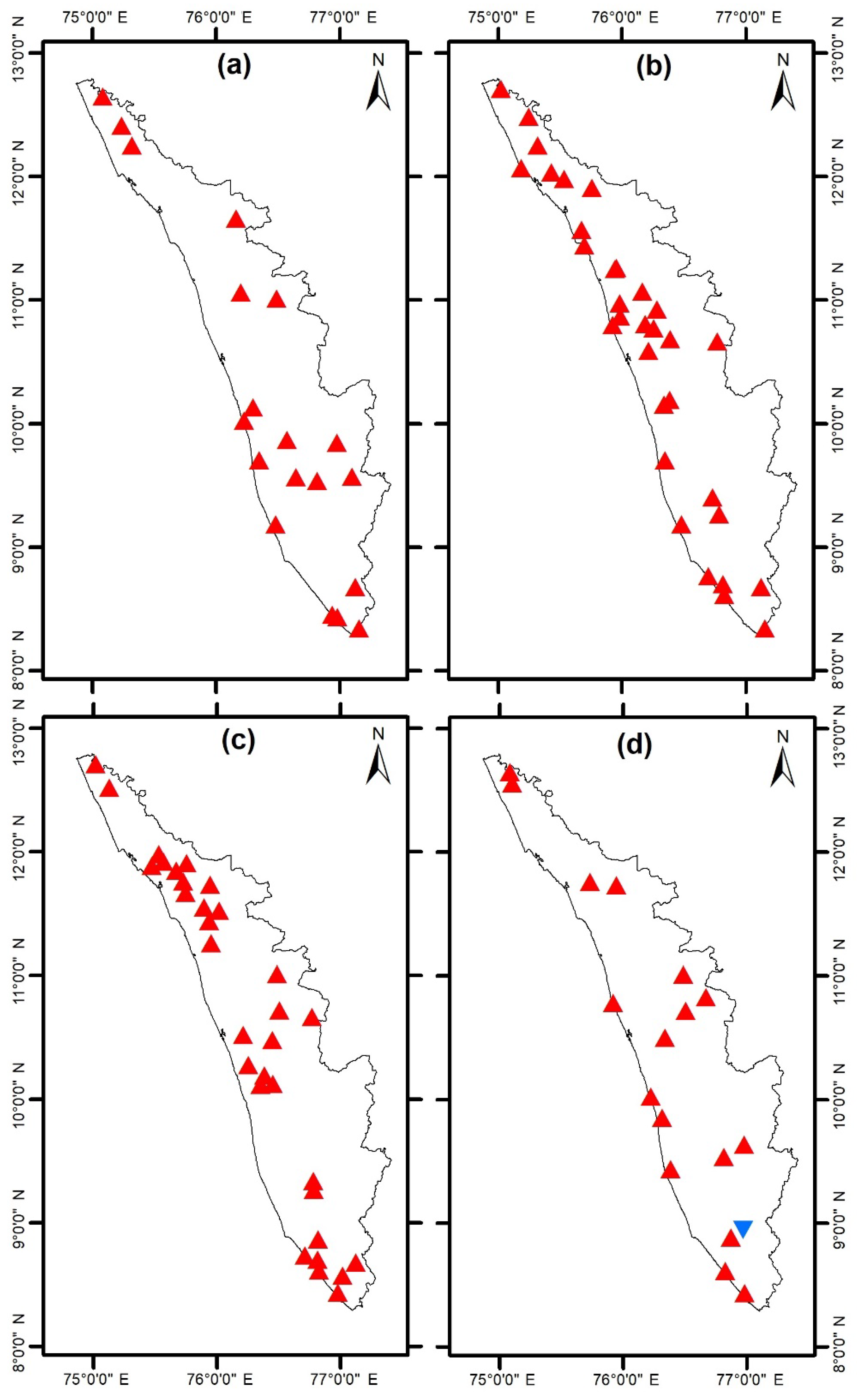
3.4. Dynamic Layers Trend Analysis

The key elements in determining climatological changes and the scenario of global warming are temperature and rainfall. Soil moisture and normalized difference vegetation index are the indicators that help to bind the water beneath the Earth surface. Using the possible groundwater level trend sites 19-32-26-18, the BEAST is run for the dynamic layer dataset received over the JAAN months.

3.4.1. Climatological Factors

Increased precipitation should potentially result in more water being available. That is, the upward trend in rainfall should be followed by a downward trend in groundwater levels. As for temperature, the upward tendency should translate into an upward trend in groundwater levels. The rainfall trend results for the 19-32-26-18 well locations are shown in Figure 9. Blue triangles indicate the increasing trend in rainfall, while red triangles indicate the decreasing trend in rainfall. The results of the rainfall trend for the month of January showed a positive trend in nine well locations, a negative trend in nine locations, and a zero trend in the Cherthalai location. Most of the increasing trends are found towards the southern part of Kerala, while the decreasing trend is scattered over the region. During the month of April, the increase in rainfall trends resulted to 14 positive trends, 17 negative trends, and a zero trend at the Kottanadu well location. It is observed that more than half of the wells had an increasing rainfall trend during April. The converse is the situation during the monsoon month of August, which can be viewed as an impact of climate change. A total of 17 negative trend and 9 positive trend rainfall locations were observed during August. Only the Ponnani1 well location showed a negative rainfall trend in November, while the remaining 17 wells showed an increase. The rainfall trends provide a rough idea of the recharge option available.

Temperature is an influential parameter to humidity and rainfall. Over the feasible locations of 19-32-26-18, an increasing temperature trend is observed in the majority of the wells. The temperature trend results are shown in Figure 10. Red triangles denote increasing temperature and reverse influence to groundwater levels. The blue triangle represents decreasing temperature, which is helpful in increasing water quantity. Out of 18 locations during the month of November, only the Ailara well location showed a decreasing trend in temperature. The results validate the global warming scenario experienced over recent decades.

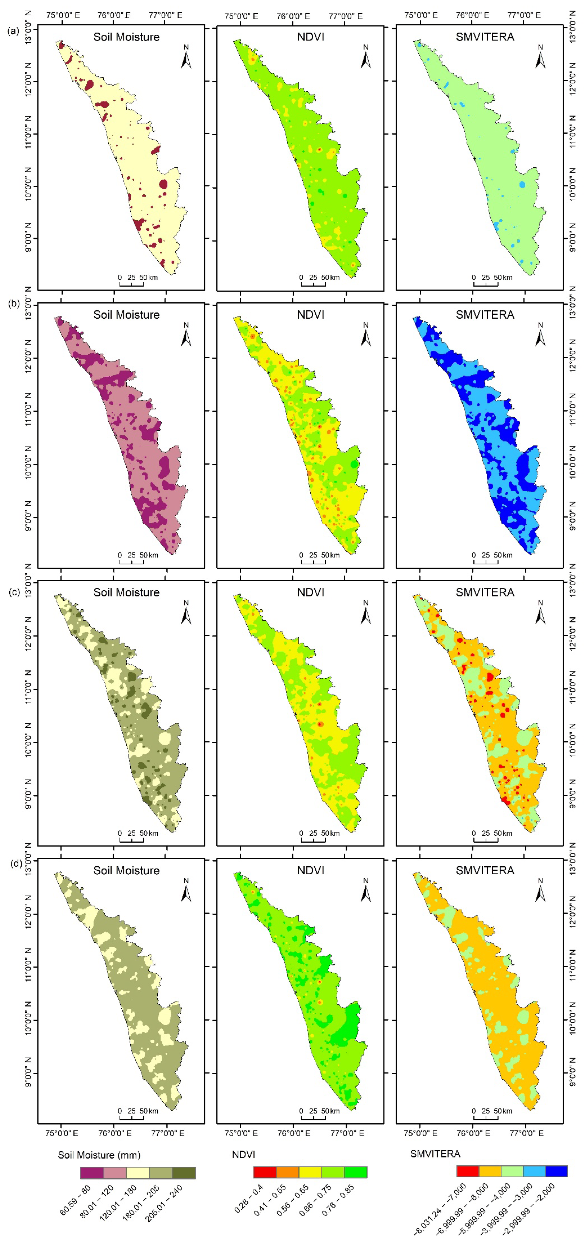
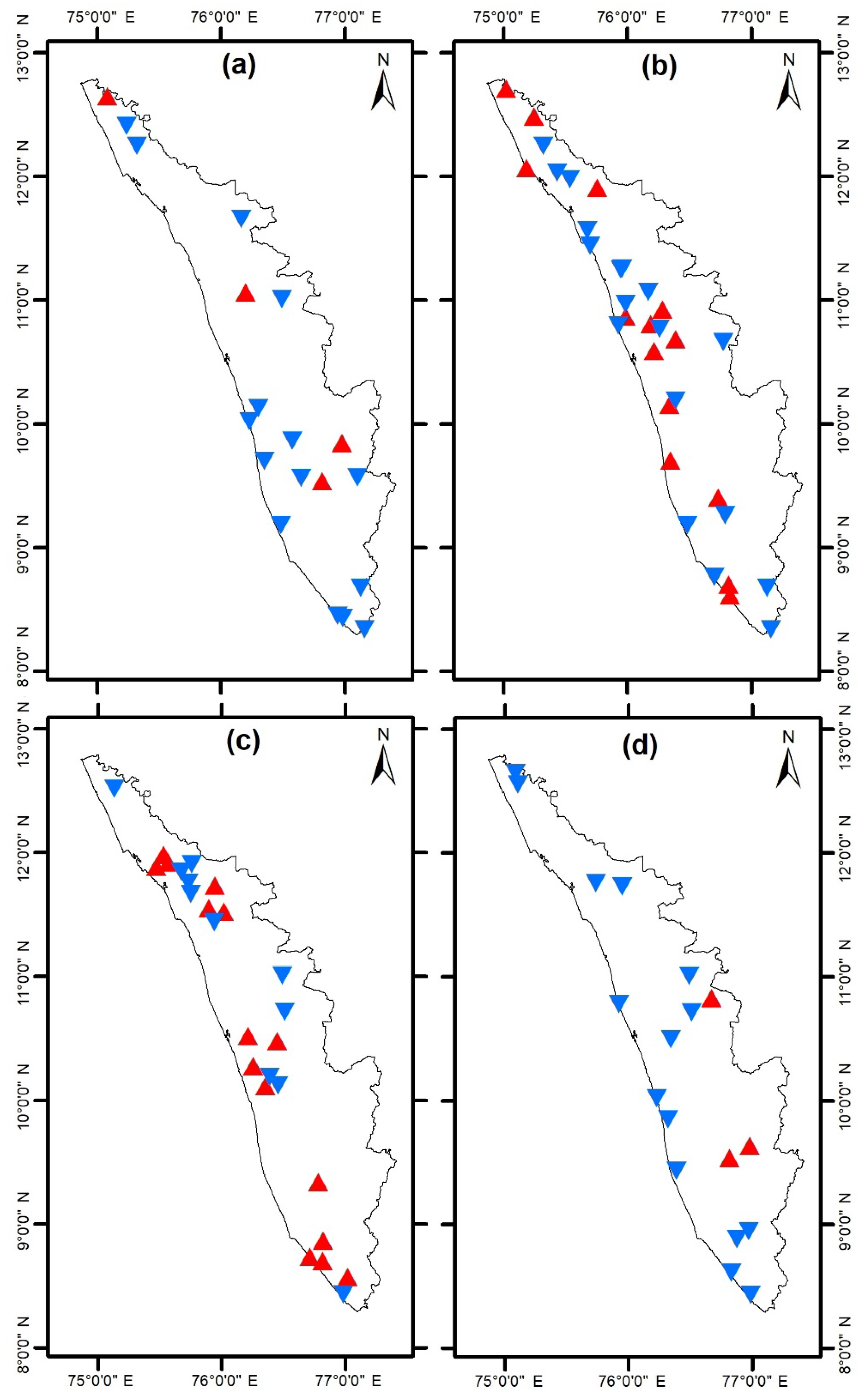
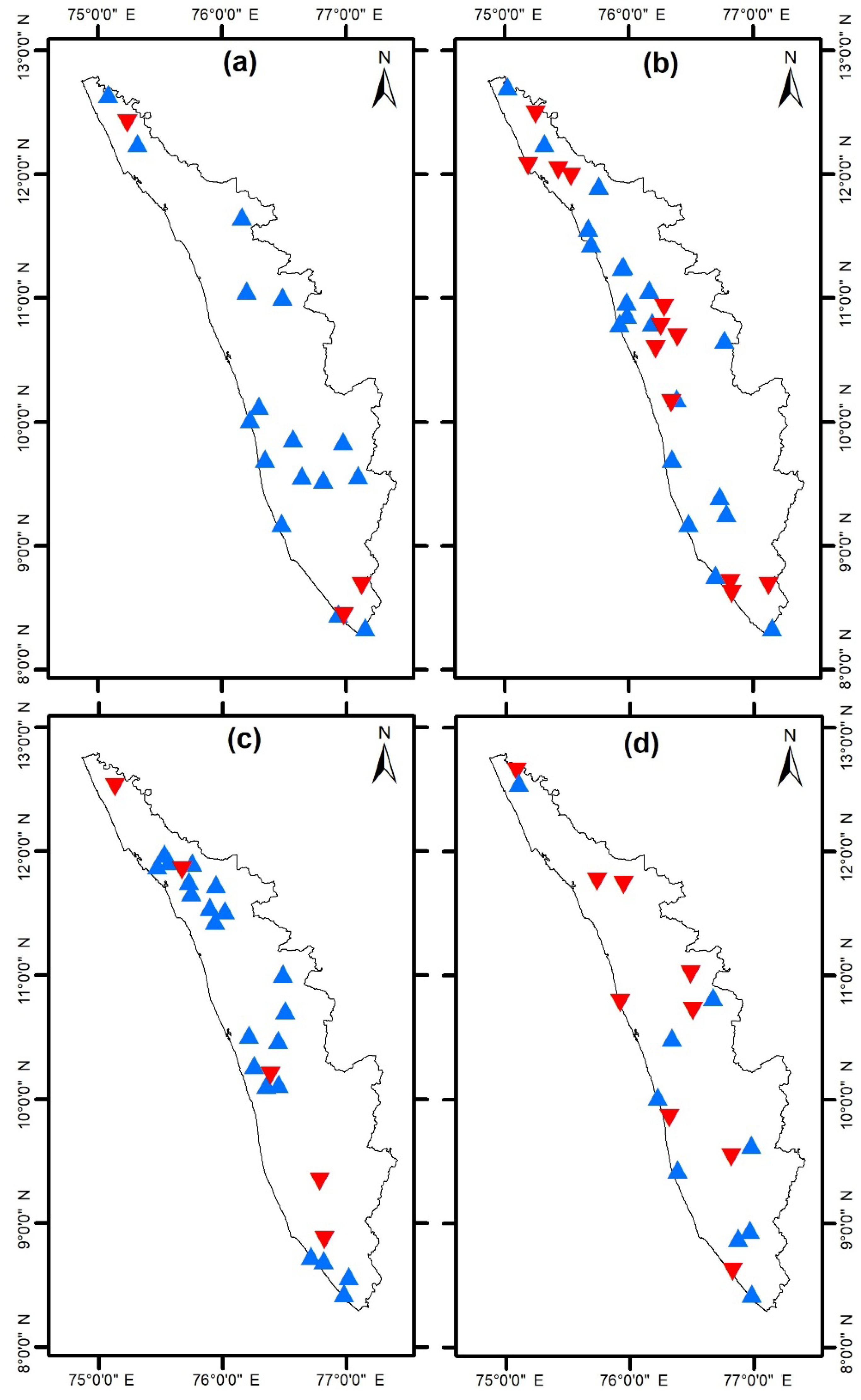
3.4.2. Soil Moisture and NDVI

The soil moisture has an inverse relation with the allowance of water getting recharged below the Earth’s surface. As the moisture content increases, the water gets trapped on the Earth’s surface and is not able to pass through. The soil moisture trend results on 19-32-26-18 locations are shown in Figure 11. During the month of January, 3 well locations—namely Angadimogar, Tachinganedam, and Kuvapalli and Idukki—showed increasing trends, while the remaining 16 wells showed decreasing soil moisture trends. In month of April, 18 wells showed negative trends and 14 wells exhibited decreasing trends in soil moisture. A greater number of positive trends were observed in the month of August, which correspond to 15 well locations. However, in the month of November, the majority of the wells had decreasing trends, while the Kuvapalli, Malampuzha, and Elappara locations showed increasing trends. In short, a lower number of locations had negative trends in January and November.

The normalized difference vegetation index has direct influence on groundwater levels. In the month of January, three well locations—namely Poonkulam, Rajapuram, and Maruthamala—showed decreasing trends in NDVI. These wells are located in the northern and southern parts of Kerala. The remaining 16 wells have increasing trends for NDVI. Similarly, a greater number of wells have positive trends in April and August as well. This amounts to 20 wells in April and 21 wells in August with positive NDVI trends, while 12 wells in April showed negative trends. The wells Akkal, Kannavam, Muliyar, Angamalil, and Elanthur exhibited decreasing NDVI trends during the month of August. In the month of November, nine wells each showed negative and positive trends. The NDVI trend results on 19-32-26-18 locations are shown in Figure 12. Blue triangles indicate increasing trends and thereby contributes to increasing water quantity, while red triangles indicate the decreasing NDVI trends and hence decreases in the possibility of water recharge.

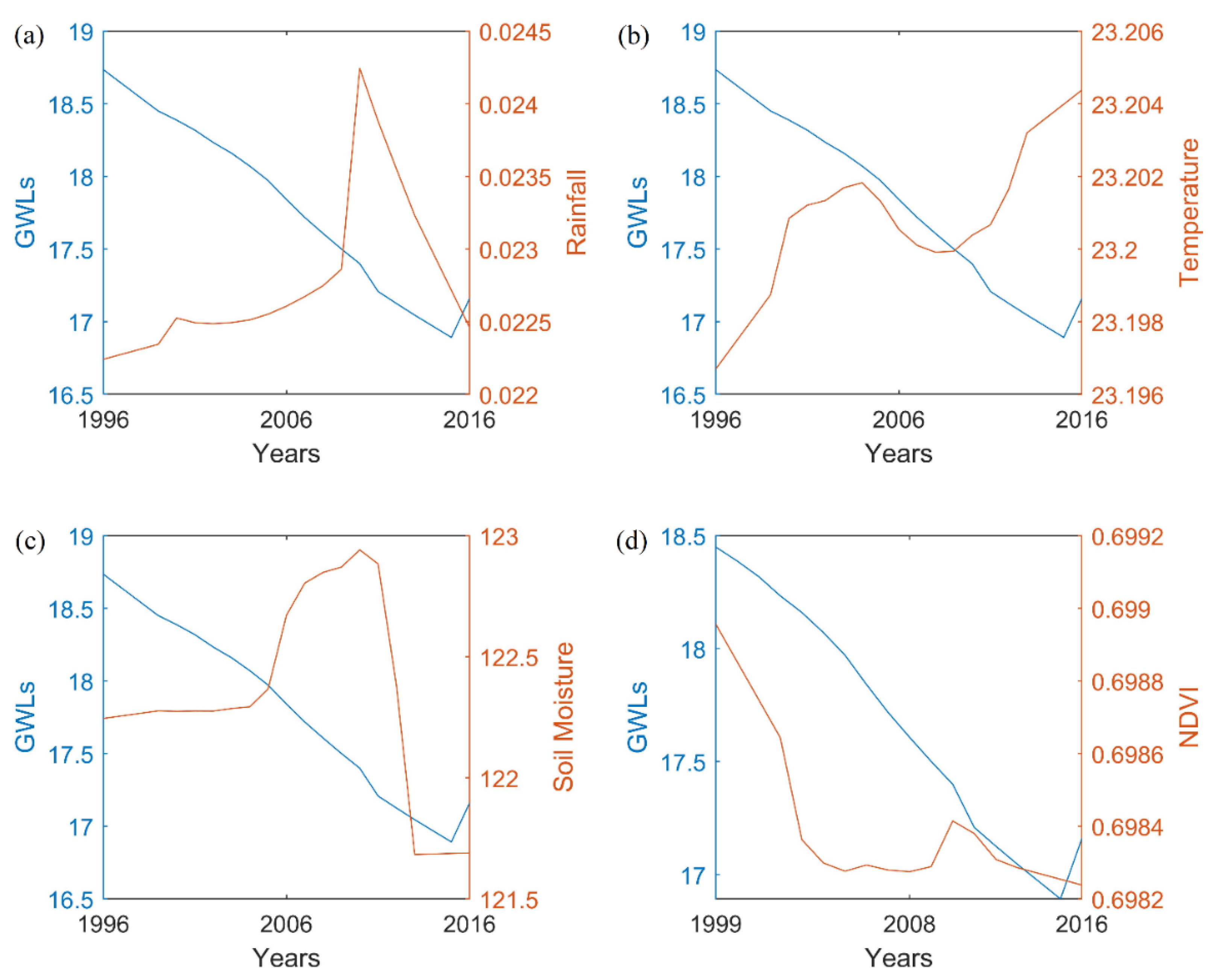
3.5. Dynamic Layer Trend in Accordance with Groundwater Level

Out of the dynamic variables considered, rainfall and NDVI have a direct influence on the water holding capacity, while temperature and soil moisture have an inverse relationship. That is, if there is an increasing trend of rainfall, the groundwater level in that particular location is expected to increase, considering all of the other dynamics are already apt. The case is similar for NDVI: the increasing trend should contribute to increasing water availability. In terms of positive and negative trends, a positive trend in rainfall or NDVI will help to create a negative trend in groundwater levels. When the relationship is viewed from the inversely related variables, namely temperature and soil moisture, the positive trend should result in a positive trend in the groundwater levels. If these conditions are met, then in those locations, the changes in water levels could be explained by the dynamic layers and can be termed as matching locations. If the conditions are not met, these non-matching well locations need to be studied in detail with the help of the static layers to understand the structure beneath the surface.

Table 3. Trend matching (M) and non-matching (NM) sites of dynamic layers and index with respect to the groundwater level trend.

Month	RA		TE		SM		VI		Index
	M	NM	M	NM	M	NM	M	NM	M	NM
Jan	6+5	8	0+9	9	3+9	7	1+8	10	9+4	6
Apr	11+4	17	0+7	25	15+4	13	15+2	15	20+1	11
Aug	1+12	13	0+20	6	0+10	16	5+4	17	1+13	12
Nov	4+0	14	0+12	6	5+3	10	4+8	6	5+2	11

shows the number of matching and non-matching well locations using the trends compared. The matching locations have been further identified from increasing and decreasing trend, respectively. A plot of the groundwater level for the month of January versus each of the dynamic variables of a random well is shown in Figure 13. From the double plot it can be observed that it is difficult to conclude a single statement or inference.

The rainfall trend showed matching in 11, 15, 13, and 4 locations, respectively, in the JAAN months, which equate to approximately 57.9%, 46.9%, 50%, and 22.2%, respectively. In the case of temperature, more matching percentages were obtained in the months of August and November. The number of matching wells is 9, 7, 20, and 12, which is 47.4%, 21.9%, 76.9%, and 66.4% of the considered wells in month order. The soil moisture percentage matching is the highest with 12 wells, which is approximately 63.2% of wells in January, and the lowest with 10 wells, which is approximately 38.5% of wells in August. The month of April has 59.4% of matching wells in April and 44.4% of matching wells in November for soil moisture. The NDVI matching percentages are 17.4%, 53.1%, 34.6%, and 66.7%, in the order of months. In January and April, the greatest matching percentage is for soil moisture, while for the month of August, the temperature matching percentage is higher. The month of November has shown the greatest matching percentages using temperature and NDVI. The variable-wise average matching equates to 44.25% for rainfall, 53.225% for temperature, 51.375% for soil moisture, and 50.45% for NDVI.

3.6. SMVITERA Index

Each of the dynamic layer trends analyzed with respect to the groundwater level trends could not yield greater matching percentages. This proves the complexity in determining the root cause for the increase or decrease in water level trends. An index has been developed that integrates all the dynamic layer advantages and disadvantages with regards to water-holding capacity. The index is then treated as a combined variable layer and BEAST is run on the obtained datasets. The trend results are shown in Figure 14, where blue triangles represent the increase in the index values and red triangles indicate the decrease in index values. In the month of January, the Angadimogar, Tachinganedam, Tenkara, Kuvapalli, and Parassala well locations showed negative trends in the index, while the remaining 13 wells showed increasing trends. Also in the month of April, 6 well locations—namely Thirunavaya, Ramantalai, Chelakod, Manattana, Paral, and Muligadde—showed decreasing trends, while 26 wells exhibited positive trends for the index. The month of August has 8 well locations with negative trends and 18 well locations with positive trends. The majority of the wells showed positive trends in November, while only two wells, Kuvapalli and Malampuzha, showed negative trends.

The matching percentages with the groundwater levels were also verified. That is, if the index value is increasing, the water availability is increasing, or more accurately the depth to water levels is decreasing. In short, the positive index trend and negative groundwater level trend are a match, and the negative index trend and positive groundwater level trend are a match. In the order of the months, 13, 21, 14, and 7 wells revealed matching and the percentages are 68.4%, 65.6%, 53.9%, and 38.9%. The non-matching well numbers are 6, 11, 12, and 11. The average matching for the index is approximately 56.7%, which is greater than all of the dynamic layer matching percentages individually considered. This proves that index is a better indicator to explain the level changes.

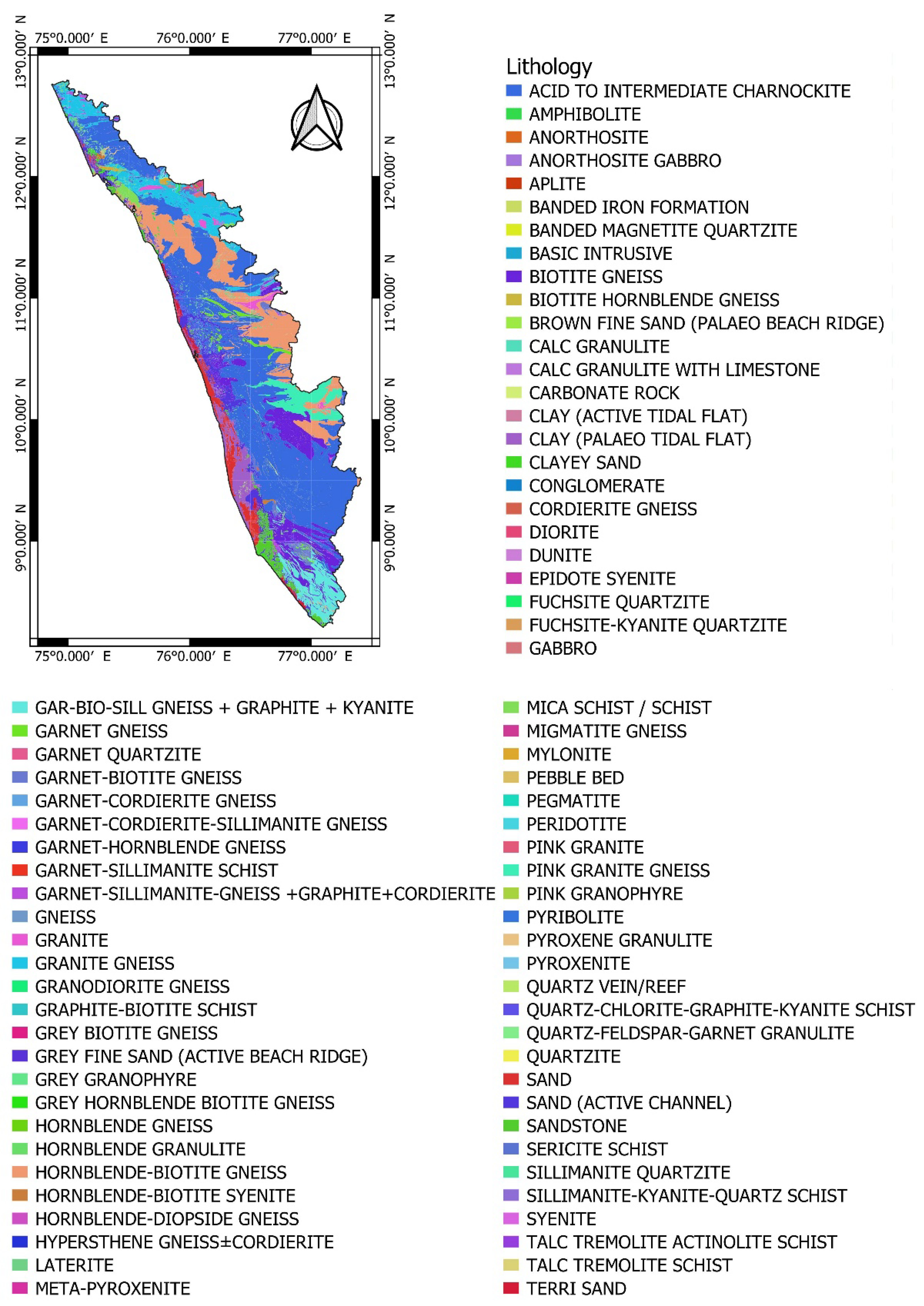
3.7. Static Layers Analysis

The lithological and geomorphological structures of the non-matching wells by the SMVITERA index is extensively studied. In the month of January, six non-matching have the Quartzite, Sand, Gar-Bio-Sill Gneiss + Graphite + Kyanite, Terri Sand, and Acid to Intermediate Charnockite as the lithology formations. Quartzite is a non-foliated metamorphic rock and does not contribute much to transfer of water. Gneiss is a foliated rock and contributes to water storage and recharge, while sand is highly permeable. Charnockite, being highly non-porous, does not allow water to pass through, and as a result does not help in groundwater recharge. The geomorphological formations are Pediment Pediplain Complex and Coastal Plain, which are promising areas of water availability. Considering all of these, the locations of over-exploitation were observed as Cherthalai, Maruthamala, and Poonthura during January.

Eleven wells showed non-matching of groundwater levels with the index. The lithological formation in these wells is Laterite, Clay, Acid to Intermediate Charnockite, Sand, Granite, Garnet Gneiss, Hornblende-Biotite Gneiss, Granite Gneiss, and Terri Sand. The geomorphological formations are Pediment Pediplain Complex, Coastal Plain, and Low Dissected Plateau, which are promising areas of water availability. The identified drying wells are Cherthalai, Shoranur, Angamali1, Palghat, and Murukumpuzha (R1) during April. Similarly, Pudukayam, Perambra, Tenkara, Kannavam, Muliyar, and Vallom1 wells are found to be overly exploited during the month of August as the lithological and geomorphological formations still have sufficient permeability. The over-exploited wells during the month of November were observed to be Tholanur, Pudukayam, Tenkara, Manamangalam, Ailara, Murukumpuzha (R1), and Chadayamangalam1.

4. Discussions

It is seldom easy to explain an inference from the variations in groundwater levels. The greatest depth to groundwater level may be a result of the area’s decreased water storage capacity or over-exploitation. The underlying problem must be investigated in order to identify whether a well is drying up and whether this has changed the water table. This study is carried out to determine the relationship between the groundwater levels, which also experience dynamic changes over the years and considered months, and the dynamic variables of surface factors, such as soil moisture and normalized difference vegetation index, and climatological factors, such as temperature and rainfall. This work has used the Bayesian Ensemble algorithm to determine trends rather than usual trend analysis techniques, such as the Mann–Kendall trend test and its modified variants or innovative trend analysis method. This work shows that groundwater level patterns can be very effectively described by BEAST, even though the applied method has not yet been employed to ascertain level trends.

Studies examining trends in groundwater levels over Kerala are few and far between. For the years 2008 to 2013, Sajeena and Kurien examined the groundwater hydrograph for the Kadalundi river basin, Malappuram district, and Kerala [76]. The water table generally rose from June to September and fell from October to May, according to observations. The findings showed that groundwater levels in the Kottakkal, Marakkara, and Tanur localities are unrelated to rainfall. Tachinganedam, Mudikode, and Kottakkal are the points where our study and the Kadalundi river basin converge. The depth of the groundwater at the Tachinganedam well location increased in January, while the depth of the groundwater at the latter well locations decreased in April. The results of the comparative study are consistent with the Tachinganedam well site, and it’s possible that throughout the subsequent years, the features of the remaining wells have altered. The water table has risen although rainfall has been trending downward in the Kottakkal well location. This is uncorrelated as there is an obvious trend mismatch. According to the groundwater potential assessment study by Jayasankar and Babu, the districts of Kannur, Wayanad, and Idukki have critical water resource quantities for the decades 1989 to 1999 and 1999 to 2009 [77]. The intersection wells in our study are Idukki, Vandiperiyar, and Elappara from Idukki district; Minangadi, Lakkidi, and Vellamuda from Wayand district; and Vayyakara, Ramantalai, Irikkur, Pukkundu, Manattana, Mattanur, Kannavam, and Chakkarakkale from Kannur district. Groundwater levels decreased in the Idukki, Vandiperiyar, Minangadi, and Vayyakara well locations in January. The depth to groundwater levels also decreased in April at the well locations in Vayyakara, Ramantalai, Irikkur, Pukkundu, and Manattana. The Lakkidi well location showed a declining trend in August, whereas the well locations in Vellamuda, Irikkur, Manattana, Mattanur, Kannavam, and Chakkarakkale showed an upward trend. Elappara and Vellamuda displayed a growing trend in the month of November. According to the report, the majority of well locations experienced a decrease in the water table in August and November, but experienced an increase in January and April. While the situation has marginally improved during the winter and pre-monsoon seasons, the trends are still being followed in the monsoon and post-monsoon seasons. Due to the location-based methodology used in this study, there is some inconsistency in the overall district or state comparisons.

The study by Jagadeesh and Anupama over the Bharathapuzha river basin is to determine rainfall trend analysis using the Mann–Kendall test [78]. The four rain gauge stations looked at were Eruthempathy, Thrithala, and the Malampuzha dam. Except at the Eruthempathy location, the study’s results showed a downward trend in rainfall during the northeast monsoon. Our study location coincides with the Malampuzha well, where we have seen increasing rainfall trends. In Kerala state, there were no discernible rainfall patterns during the annual, autumn, spring, summer, or winter according to Jaman et al. [79]. When Sai and Joseph used the Mann–Kendall trend test to assess the rainfall trends in the Pattambi region, they found negative Z values in the months of January, June, July, August, and November [80]. According to our investigation, April saw a favorable trend in rainfall at the Pattambi well location, which was consistent with previous findings. The Vamanapuram river basin’s rainfall patterns from 1984 to 2013 were examined by Berma and John [81]. For the months of January, February, May, and August, negative Z values were found. The Maruthamala and Attingal wells in our study are located in the basin. Maruthamala displayed an upward trend in January, whereas Attingal displayed a descending trend in August. Attingal exhibited a declining trend in April, whereas Maruthamala showed an upward trend. The month of August coincides with the findings of our study.

Nearly all of the well locations analyzed for this study had rising trends in average temperatures. Similar results were seen in other studies that covered the state of Kerala. Anjali and Roshni [82] attempted to relate changes in Kerala’s forest cover to rainfall and land surface temperature (LST) using satellite data. Between 2000 and 2019, the minimum and maximum LST significantly increased as a result of the Mann–Kendall trend. The patterns of climate change over Kerala’s Bharathapuzha river basin since 1900 were examined by George and Athira [83]. Both the monthly average temperature and the monthly lowest temperature showed a consistent long-term upward trend. Using the Mann–Kendall trend test, Varughese et al. [84] examined historical patterns in climate change over the same basin from 1951 to 2013. Mean, maximum, and minimum temperature trends all indicated a noticeable rise over time. Subash and Sikka [85] looked into India’s temperature and rainfall trends. The findings indicated an upward trend in the yearly maximum temperature. Over 15 basins in India, Jain and Kumar examined the temperature and rainfall patterns. The findings showed that temperatures were on the rise at the majority of the stations in southern India. The trend analysis of the mean maximum and mean minimum temperature over 13 observatories in Kerala state was conducted by Kabbilawsh et al. [86]. While the mean lowest temperature over Alappuzha indicated a declining trend, the Mann–Kendall test revealed an increase in nine places.

There aren’t many studies on NDVI and soil moisture trends over Kerala and India. Bhimala et al. [87] examined the soil moisture, rainfall, and land use and cover data in India. South and northwest India both experienced an increase in soil moisture. Parida et. al. [88] investigated the greening and browning trends of the vegetation in India. The study came to the conclusion that the southern peninsula’s vegetation and croplands were no longer greening. Chakraborty et al. [89] used NDVI to evaluate the changes in seasonal greenness across different forest types in India. In tropical moist deciduous forests, the most significant negative changes were discovered.

The acquired results are consistent with the majority of studies, but some locations show different results. This can be explained by the possibility that trends have shifted over unaccounted years.

5. Conclusions

The most popular trend analysis on hydro-climatological variables is the linear and non-parametric Mann–Kendall trend test. The question of the existence of monotonic linearity have prompted to apply other methods like the Bayesian Ensemble Algorithm to the recent researches. This study has used the Bayesian method to examine the variations in groundwater levels over 385 wells across Kerala state during the JAAN months for 21 years from 1996 to 2016. The variations were obtained using an inference in the form of the percentage area under the probability curve for the trend changes to be positive, zero, and negative. The results showed variations in groundwater levels in 19, 26, 32, and 18 well sites. From the viewpoint of climatological variables, such as temperature and rainfall, as well as surface characteristics, such as soil moisture and normalized differential vegetation index, the groundwater levels had to be studied in detail. The matching trend percentages in terms of the relationship with the variables are identified. These matching trend percentages account to about 63.2% by Soil Moisture during January, 59.4% by Soil Moisture in April, 76.9% by Temperature in August, and 66.7% equally by Temperature and Normalized Difference Vegetation Index in November. It is observed that there was no reliance on a specific variable or a particular month in the trend analysis of these dynamic layers in connection to changes in groundwater level. This prompted the creation of the SMVITERA index, which is based on these dynamic factors. The developed index has a higher average proportion of roughly 56.7% matching, according to analysis of the matching percentages of each layer individually and collectively. The individual average matching percentages were observed to be 44.25% for Rainfall, 53.23% for Temperature, 51.38% for Soil Moisture, and 50.45% for Normalized Difference Vegetation Index. The static properties of the non-matching well locations were investigated. The site has been deemed overexploited if the lithological and geomorphologic properties continue to influence the amount of water while the trend result is positive. Identification and maintenance of these places are required in a predicted-to-be water-scarce Earth.

References

1. Varma, A. Groundwater Resource and Governance in Kerala Groundwater Resource and Governance in Kerala: Status, Issues and Prospects; Forum Policy Dialogue Water Conflicts: Pune, India, 2017. [Google Scholar]
2. Pullare, N.; Ground, C.; Board, W. Changes in Ground Water Utilization in Kerala—Causes & Consequences. In Proceedings of the 4th National Ground Water Congress, Kerala, India, January 2012. [Google Scholar] [CrossRef]
3. Ziolkowska, J.R.; Reyes, R. Groundwater Level Changes Due to Extreme Weather-an Evaluation Tool for Sustainable Water Management. Water 2017, 9, 117. [Google Scholar] [CrossRef] [Green Version]
4. Hua, Z.; Cheng, W.; Yi, S.; Jiang, Q. Geostatistical Analysis of Spatial and Temporal Variations of Groundwater Depth in Shule River. In Proceedings of the 2009 WASE International Conference on Information Engineering (ICIE 2009), Taiyuan, China, 10–11 July 2009; Volume 2, pp. 453–457. [Google Scholar]
5. Bhanja, S.N.; Mukherjee, A. In Situ and Satellite-Based Estimates of Usable Groundwater Storage across India: Implications for Drinking Water Supply and Food Security. Adv. Water Resour. 2019, 126, 15–23. [Google Scholar] [CrossRef]
6. Bhanja, S.N.; Mukherjee, A.; Saha, D.; Velicogna, I.; Famiglietti, J.S. Validation of GRACE Based Groundwater Storage Anomaly Using In-Situ Groundwater Level Measurements in India. J. Hydrol. 2016, 543, 729–738. [Google Scholar] [CrossRef]
7. Machiwal, D.; Jha, M.K.; Mal, B.C. Assessment of Groundwater Potential in a Semi-Arid Region of India Using Remote Sensing, GIS and MCDM Techniques. Water Resour. Manag. 2011, 25, 1359–1386. [Google Scholar] [CrossRef]
8. Mengistu, H.A.; Demlie, M.B.; Abiye, T.A. Review: Groundwater Resource Potential and Status of Groundwater Resource Development in Ethiopia. Hydrogeol. J. 2019, 27, 1051–1065. [Google Scholar] [CrossRef]
9. Srivastava, S.; Singh, J.; Shirsath, P.B. Sustainability of Groundwater Resources at the Subnational Level in the Context of Sustainable Development Goals. Agric. Econ. Res. Rev. 2018, 31, 79. [Google Scholar] [CrossRef] [Green Version]
10. Koundouri, P. Potential for Groundwater Management: Gisser-Sanchez Effect Reconsidered. Water Resour. Res. 2004, 40, W06S16. [Google Scholar] [CrossRef] [Green Version]
11. Thakur, G.S.; Thomas, T. Analysis of Groundwater Levels for Detection of Trend in Sagar District, Madhya Pradesh. J. Geol. Soc. India 2011, 77, 303–308. [Google Scholar] [CrossRef] [Green Version]
12. Knapp, K.C.; Weinberg, M.; Howitt, R.; Posnikoff, J.F. Water Transfers, Agriculture, and Groundwater Management: A Dynamic Economic Analysis. J. Environ. Manag. 2003, 67, 291–301. [Google Scholar] [CrossRef] [PubMed]
13. Ali, R.; Rashid Abubaker, S.; Othman Ali, R. Spatio-Temporal Pattern in the Changes in Availability and Sustainability of Water Resources in Afghanistan View Project Water Resources Problem in Huai River Basin View Project Trend Analysis Using Mann-Kendall, Sen’s Slope Estimator Test and Innovative. Int. J. Eng. Technol. 2019, 8, 110–119. [Google Scholar] [CrossRef]
14. Xing, L.; Huang, L.; Chi, G.; Yang, L.; Li, C.; Hou, X. A Dynamic Study of a Karst Spring Based on Wavelet Analysis and the Mann-Kendall Trend Test. Water 2018, 10, 698. [Google Scholar] [CrossRef] [Green Version]
15. Hamidov, A.; Khamidov, M.; Ishchanov, J. Impact of Climate Change on Groundwater Management in the Northwestern Part of Uzbekistan. Agronomy 2020, 10, 1173. [Google Scholar] [CrossRef]
16. Dinpashoh, Y. Trend Analysis of Groundwater Level, Using Mann-Kendall Non Parametric Method (Case Study: Tabriz Plain). J. Water Soil Sci. 2019, 23, 335–348. [Google Scholar] [CrossRef] [Green Version]
17. Meggiorin, M.; Passadore, G.; Bertoldo, S.; Sottani, A.; Rinaldo, A. Assessing the Long-Term Sustainability of the Groundwater Resources in the Bacchiglione Basin (Veneto, Italy) with the Mann–Kendall Test: Suggestions for Higher Reliability. Acque Sotter. Ital. J. Groundw. 2021, 10, 35–48. [Google Scholar] [CrossRef]
18. Wilopo, W.; Putra, D.P.E.; Hendrayana, H. Impacts of Precipitation, Land Use Change and Urban Wastewater on Groundwater Level Fluctuation in the Yogyakarta-Sleman Groundwater Basin, Indonesia. Environ. Monit. Assess. 2021, 193, 76. [Google Scholar] [CrossRef] [PubMed]
19. Ndlovu, M.S.; Demlie, M. Statistical Analysis of Groundwater Level Variability across KwaZulu-Natal Province, South Africa. Environ. Earth Sci. 2018, 77, 739. [Google Scholar] [CrossRef]
20. Valois, R.; MacDonell, S.; Núñez Cobo, J.H.; Maureira-Cortés, H. Groundwater Level Trends and Recharge Event Characterization Using Historical Observed Data in Semi-Arid Chile. Hydrol. Sci. J. 2020, 65, 597–609. [Google Scholar] [CrossRef]
21. Goyal, S.K.; Chaudhary, B.S.; Singh, O.; Sethi, G.K.; Thakur, P.K. Variability Analysis of Groundwater Levels—AGIS-Based Case Study. J. Indian Soc. Remote Sens. 2010, 38, 355–364. [Google Scholar] [CrossRef]
22. Anand, B.; Karunanidhi, D.; Subramani, T.; Srinivasamoorthy, K.; Suresh, M. Long-Term Trend Detection and Spatiotemporal Analysis of Groundwater Levels Using GIS Techniques in Lower Bhavani River Basin, Tamil Nadu, India. Environ. Dev. Sustain. 2020, 22, 2779–2800. [Google Scholar] [CrossRef]
23. Panda, D.K.; Mishra, A.; Kumar, A.; Mishra, D.K.; Kumar, A. Quantification of Trends in Groundwater Levels of Gujarat in Western India. Hydrol. Sci. J. 2012, 57, 1325–1336. [Google Scholar] [CrossRef]
24. Krishan, G.; Rao, M.S.; Loyal, R.S.; Lohani, A.K.; Tuli, N.K.; Takshi, K.S.; Kumar, C.P.; Semwal, P.; Kumar, S. Groundwater Level Analyses of Punjab, India: A Quantitative Approach. Octa J. Environ. Res. 2014, 2, 221–226. [Google Scholar]
25. Sishodia, R.P.; Shukla, S.; Graham, W.D.; Wani, S.P.; Garg, K.K. Bi-Decadal Groundwater Level Trends in a Semi-Arid South Indian Region: Declines, Causes and Management. J. Hydrol. Reg. Stud. 2016, 8, 43–58. [Google Scholar] [CrossRef] [Green Version]
26. Tirkey, A.S.; Pandey, A.C.; Nathawat, M.S. Groundwater Level and Rainfall Variability Trend Analysis Using GIS in Parts of Jharkhand State ( India ) for Sustainable Management of Water Resources. Int. Res. J. Environ. Sci. 2012, 1, 24–31. [Google Scholar]
27. Dinpashoh, Y.; Mirabbasi, R.; Jhajharia, D.; Abianeh, H.Z.; Mostafaeipour, A. Effect of Short-Term and Long-Term Persistence on Identification of Temporal Trends. J. Hydrol. Eng. 2014, 19, 617–625. [Google Scholar] [CrossRef]
28. Kumar, S.; Merwade, V.; Kam, J.; Thurner, K. Streamflow Trends in Indiana: Effects of Long Term Persistence, Precipitation and Subsurface Drains. J. Hydrol. 2009, 374, 171–183. [Google Scholar] [CrossRef]
29. Drápela, K.; Drápelová, I.; Drápela, D.I.K. Application of Mann-Kendall Test and the Sen’s Slope Estimates for Trend Detection in Deposition Data from Bílý Kříž (Beskydy Mts., the Czech Republic) 1997–2010. Beskydy 2011, 4, 133–146. [Google Scholar]
30. Patakamuri, S.K.; Muthiah, K.; Sridhar, V. Long-Term Homogeneity, Trend, and Change-Point Analysis of Rainfall in the Arid District of Ananthapuramu, Andhra Pradesh State, India. Water 2020, 12, 211. [Google Scholar] [CrossRef] [Green Version]
31. Satish Kumar, K.; Venkata Rathnam, E. Analysis and Prediction of Groundwater Level Trends Using Four Variations of Mann Kendall Tests and ARIMA Modelling. J. Geol. Soc. India 2019, 94, 281–289. [Google Scholar] [CrossRef]
32. Swain, S.; Sahoo, S.; Taloor, A.K.; Mishra, S.K.; Pandey, A. Exploring Recent Groundwater Level Changes Using Innovative Trend Analysis (ITA) Technique over Three Districts of Jharkhand, India. Groundw. Sustain. Dev. 2022, 18, 100783. [Google Scholar] [CrossRef]
33. Zakwan, M. Trend Analysis of Groundwater Level Using Innovative Trend Analysis. In Groundwater Resources Development and Planning in the Semi-Arid Region; Springer: Cham, Switzerland, 2021; pp. 389–405. [Google Scholar]
34. Abbas, M.; Arshad, M.; Shahid, M.A. Charectarization of Groundwater Level Zones Using Innovative Trend & Regression Analysis: Case Study at Rechna Doab-Pakistan. Available online: https://www.researchsquare.com/article/rs-2140740/v1 (accessed on 5 November 2022).
35. Li, J.; Li, Z.L.; Wu, H.; You, N. Trend, Seasonality, and Abrupt Change Detection Method for Land Surface Temperature Time-Series Analysis: Evaluation and Improvement. Remote Sens. Environ. 2022, 280, 113222. [Google Scholar] [CrossRef]
36. Yang, X.; Tian, S.; You, W.; Jiang, Z. Reconstruction of Continuous GRACE/GRACE-FO Terrestrial Water Storage Anomalies Based on Time Series Decomposition. J. Hydrol. 2021, 603, 127018. [Google Scholar] [CrossRef]
37. Xu, X.; Yang, J.; Ma, C.; Qu, X.; Chen, J.; Cheng, L. Segmented Modeling Method of Dam Displacement Based on BEAST Time Series Decomposition. Measurement 2022, 202, 111811. [Google Scholar] [CrossRef]
38. Tingwei, C.; Tingxuan, H.; Bing, M.; Fei, G.; Yanfang, X.; Rongjie, L.; Yi, M.; Jie, Z.; Tingwei, C.; Tingxuan, H.; et al. Spatiotemporal Pattern of Aerosol Types over the Bohai and Yellow Seas Observed by CALIOP. Infrared Laser Eng. 2021, 50, 20211030–20211031. [Google Scholar] [CrossRef]
39. Duke, N.C.; Mackenzie, J.R.; Canning, A.D.; Hutley, L.B.; Bourke, A.J.; Kovacs, J.M.; Cormier, R.; Staben, G.; Lymburner, L.; Ai, E. ENSO-Driven Extreme Oscillations in Mean Sea Level Destabilise Critical Shoreline Mangroves—An Emerging Threat. PLoS Clim. 2022, 1, e0000037. [Google Scholar] [CrossRef]
40. Zannat, F.; Islam, A.R.M.T.; Rahman, M.A. Spatiotemporal Variability of Rainfall Linked to Ground Water Level under Changing Climate in Northwestern Region, Bangladesh. Eur. J. Geosci. 2019, 1, 35–56. [Google Scholar] [CrossRef]
41. Shaji, E. Groundwater Quality Management in Kerala. Int. Inte-Res. J. 2013, 3, 63–68. [Google Scholar]
42. Tabari, H.; Nikbakht, J.; Shifteh Some’e, B. Investigation of Groundwater Level Fluctuations in the North of Iran. Environ. Earth Sci. 2011, 66, 231–243. [Google Scholar] [CrossRef]
43. Oleszczuk, R.; Jadczyszyn, J.; Gnatowski, T.; Brandyk, A. Variation of Moisture and Soil Water Retention in a Lowland Area of Central Poland—Solec Site Case Study. Atmosphere 2022, 13, 1372. [Google Scholar] [CrossRef]
44. Naga Rajesh, A.; Abinaya, S.; Purna Durga, G.; Lakshmi Kumar, T.V. Long-Term Relationships of MODIS NDVI with Rainfall, Land Surface Temperature, Surface Soil Moisture and Groundwater Storage over Monsoon Core Region of India. Arid L. Res. Manag. 2022, 1–20. [Google Scholar] [CrossRef]
45. Halder, S.; Roy, M.B.; Roy, P.K. Analysis of Groundwater Level Trend and Groundwater Drought Using Standard Groundwater Level Index: A Case Study of an Eastern River Basin of West Bengal, India. SN Appl. Sci. 2020, 2, 507. [Google Scholar] [CrossRef] [Green Version]
46. Sahoo, S.; Swain, S.; Goswami, A.; Sharma, R.; Pateriya, B. Assessment of Trends and Multi-Decadal Changes in Groundwater Level in Parts of the Malwa Region, Punjab, India. Groundw. Sustain. Dev. 2021, 14, 100644. [Google Scholar] [CrossRef]
47. Babre, A.; Kalvāns, A.; Avotniece, Z.; Retiķe, I.; Bikše, J.; Jemeljanova, K.P.M.; Zelenkevičs, A.; Dēliņa, A. The Use of Predefined Drought Indices for the Assessment of Groundwater Drought Episodes in the Baltic States over the Period 1989–2018. J. Hydrol. Reg. Stud. 2022, 40, 101049. [Google Scholar] [CrossRef]
48. Guo, M.; Yue, W.; Wang, T.; Zheng, N.; Wu, L. Assessing the Use of Standardized Groundwater Index for Quantifying Groundwater Drought over the Conterminous US. J. Hydrol. 2021, 598, 126227. [Google Scholar] [CrossRef]
49. Khaira, A.; Dwivedi, R.K. A State of the Art Review of Analytical Hierarchy Process. Mater. Today Proc. 2018, 5, 4029–4035. [Google Scholar] [CrossRef]
50. Singh, R.P.; Nachtnebel, H.P. Analytical Hierarchy Process (AHP) Application for Reinforcement of Hydropower Strategy in Nepal. Renew. Sustain. Energy Rev. 2016, 55, 43–58. [Google Scholar] [CrossRef]
51. Goepel, K.D. Comparison of Judgment Scales of the Analytical Hierarchy Process—A New Approach. Int. J. Inf. Technol. Decis. Mak. 2019, 18, 445–463. [Google Scholar] [CrossRef] [Green Version]
52. Azizkhani, M.; Vakili, A.; Noorollahi, Y.; Naseri, F. Potential Survey of Photovoltaic Power Plants Using Analytical Hierarchy Process (AHP) Method in Iran. Renew. Sustain. Energy Rev. 2017, 75, 1198–1206. [Google Scholar] [CrossRef]
53. Thanki, S.; Govindan, K.; Thakkar, J. An Investigation on Lean-Green Implementation Practices in Indian SMEs Using Analytical Hierarchy Process (AHP) Approach. J. Clean. Prod. 2016, 135, 284–298. [Google Scholar] [CrossRef]
54. Joseph, E.J.; Anitha, A.B.; Jayakumar, P.; Sushanth, C.M.; Jayakumar, K.V. Climate Change and Sustainable Water Resources Management in Kerala; Centre of Water Resources Development and Management: Kozhikode, India, 2011. [Google Scholar]
55. Huang, J.; Van Den Dool, H.M.; Georgakakos, K.P. Analysis of Model-Calculated Soil Moisture over the United States (1931-1993) and Applications to Long-Range Temperature Forecasts. J. Clim. 1996, 9, 1350–1362. [Google Scholar] [CrossRef]
56. Fan, Y.; Van Den Dool, H. Climate Prediction Center Global Monthly Soil Moisture Data Set at 0.5&deg; Resolution for 1948 to Present. J. Geophys. Res. 2004, 109, 10102. [Google Scholar] [CrossRef] [Green Version]
57. Sajjad, M.M.; Wang, J.; Abbas, H.; Ullah, I.; Khan, R.; Ali, F. Impact of Climate and Land-Use Change on Groundwater Resources, Study of Faisalabad District, Pakistan. Atmosphere 2022, 13, 1097. [Google Scholar] [CrossRef]
58. Baret, F.; Weiss, M.; Lacaze, R.; Camacho, F.; Makhmara, H.; Pacholcyzk, P.; Smets, B. GEOV1: LAI and FAPAR Essential Climate Variables and FCOVER Global Time Series Capitalizing over Existing Products. Part1: Principles of Development and Production. Remote Sens. Environ. 2013, 137, 299–309. [Google Scholar] [CrossRef]
59. León-Tavares, J.; Roujean, J.-L.; Smets, B.; Wolters, E.; Toté, C.; Swinnen, E. Correction of Directional Effects in VEGETATION NDVI Time-Series. Remote Sens. 2021, 13, 1130. [Google Scholar] [CrossRef]
60. Toté, C.; Swinnen, E.; Sterckx, S.; Clarijs, D.; Quang, C.; Maes, R. Evaluation of the SPOT/VEGETATION Collection 3 Reprocessed Dataset: Surface Reflectances and NDVI. Remote Sens. Environ. 2017, 201, 219–233. [Google Scholar] [CrossRef]
61. Toté, C.; Swinnen, E.; Sterckx, S.; Adriaensen, S.; Benhadj, I.; Iordache, M.-D.; Bertels, L.; Kirches, G.; Stelzer, K.; Dierckx, W.; et al. Evaluation of PROBA-V Collection 1: Refined Radiometry, Geometry, and Cloud Screening. Remote Sens. 2018, 10, 1375. [Google Scholar] [CrossRef] [Green Version]
62. Pai, D.; Rajeevan, M.; Sreejith, O.; Mukhopadhyay, B.; Satbha, N. Development of a New High Spatial Resolution (0.25° × 0.25°) Long Period (1901-2010) Daily Gridded Rainfall Data Set over India and Its Comparison with Existing Data Sets over the Region. Mausam 2021, 65, 1–18. [Google Scholar] [CrossRef]
63. Srivastava, A.K.; Rajeevan, M.; Kshirsagar, S.R. Development of a High Resolution Daily Gridded Temperature Data Set (1969-2005) for the Indian Region. Atmos. Sci. Lett. 2009, 10, 249–254. [Google Scholar] [CrossRef]
64. Saaty, R.W. The Analytic Hierarchy Process-What It Is and How It Is Used. Math. Model. 1987, 9, 161–176. [Google Scholar] [CrossRef] [Green Version]
65. Saaty, T.L. How to Make a Decision: The Analytic Hierarchy Process. Eur. J. Oper. Res. 1990, 48, 9–26. [Google Scholar] [CrossRef]
66. David, F.N.; Kendall, M.G. Rank Correlation Methods. J. R. Stat. Soc. Ser. A 1956, 119, 90. [Google Scholar] [CrossRef]
67. Mann, H.B. Nonparametric Tests Against Trend. Econometrica 1945, 13, 245. [Google Scholar] [CrossRef]
68. Sen, P.K. Estimates of the Regression Coefficient Based on Kendall’s Tau. J. Am. Stat. Assoc. 1968, 63, 1379–1389. [Google Scholar] [CrossRef]
69. Theil, H. A Rank-Invariant Method of Linear and Polynomial Regression Analysis, 1–2; Proceedings of the Koninklijke Nederlandse Akademie Wetenschappen, Series A Mathematical Sciences. 1950, 53, pp. 386–392, 521–525. Available online: https://www.scirp.org/(S(351jmbntvnsjt1aadkposzje))/reference/ReferencesPapers.aspx?ReferenceID=1245706 (accessed on 5 November 2022).
70. Theil, H. A Rank-Invariant Method of Linear and Polynomial Regression Analysis, 3; Proceedings of the Koninklijke Nederlandse Akademie Wetenschappen, Series A Mathematical Sciences. 1950, 53, pp. 1397–1412. Available online: https://www.scirp.org/(S(351jmbntvnsjt1aadkposzje))/reference/ReferencesPapers.aspx?ReferenceID=1245706 (accessed on 5 November 2022).
71. Zhao, K.; Wulder, M.A.; Hu, T.; Bright, R.; Wu, Q.; Qin, H.; Li, Y.; Toman, E.; Mallick, B.; Zhang, X.; et al. Detecting Change-Point, Trend, and Seasonality in Satellite Time Series Data to Track Abrupt Changes and Nonlinear Dynamics: A Bayesian Ensemble Algorithm. Remote Sens. Environ. 2019, 232, 111181. [Google Scholar] [CrossRef]
72. White, J.H.R.; Walsh, J.E.; Thoman, R.L. Using Bayesian Statistics to Detect Trends in Alaskan Precipitation. Int. J. Climatol. 2021, 41, 2045–2059. [Google Scholar] [CrossRef]
73. Verbesselt, J.; Hyndman, R.; Zeileis, A.; Culvenor, D. Phenological Change Detection While Accounting for Abrupt and Gradual Trends in Satellite Image Time Series. Remote Sens. Environ. 2010, 114, 2970–2980. [Google Scholar] [CrossRef] [Green Version]
74. Jiang, B.; Liang, S.; Wang, J.; Xiao, Z. Modeling MODIS LAI Time Series Using Three Statistical Methods. Remote Sens. Environ. 2010, 114, 1432–1444. [Google Scholar] [CrossRef]
75. Zhao, K.; Valle, D.; Popescu, S.; Zhang, X.; Mallick, B. Hyperspectral Remote Sensing of Plant Biochemistry Using Bayesian Model Averaging with Variable and Band Selection. Remote Sens. Environ. 2013, 132, 102–119. [Google Scholar] [CrossRef]
76. Sajeena, S.; Kurien, E.K. Hydrogeological Characteristics and Groundwater Scenario of Kadalundi River Basin, Malappuram District, Kerala. Trends Biosci. 2017, 10, 2193–2200. [Google Scholar]
77. Jayasankar, P.; Babu, M.N.S. An Assessment of Ground Water Potential for State of Kerala, India: A Case Study. AE Int. J. Sci. Technol. 2017, 5. [Google Scholar]
78. Jagadeesh, P.; Anupama, C. Statistical and Trend Analyses of Rainfall: A Case Study of Bharathapuzha River Basin, Kerala, India. ISH J. Hydraul. Eng. 2014, 20, 119–132. [Google Scholar] [CrossRef]
79. Jaman Basheer Ahamed, M.; Ravichandran, C.; Ebraheem, A.M.A. Analysis of Trend and Magnitude Using Mann-Kendall and Sen’s Slope Test in 115 Years Annual Rainfall Data of South India. Adv. Appl. Math. Sci. 2022, 21, 3419–3429. [Google Scholar]
80. Sai, K.V.; Joseph, A. Trend Analysis of Rainfall of Pattambi Region, Kerala. Int. J. Curr. Microbiol. Appl. Sci. 2018, 7, 3274–3281. [Google Scholar] [CrossRef]
81. Brema, J. John Anie Rainfall Trend Analysis by Mann-Kendall Test for Vamanapuram River Basin, Kerala. Int. J. Civ. Eng. Technol. 2018, 9, 1549–1556. [Google Scholar]
82. Anjali, K.; Roshni, T. Linking Satellite-Based Forest Cover Change with Rainfall and Land Surface Temperature in Kerala, India. Environ. Dev. Sustain. 2022, 24, 11282–11300. [Google Scholar] [CrossRef]
83. George, J. Long-Term Changes in Climatic Variables over the Bharathapuzha River Basin, Kerala, India. Theor. Appl. Climatol. 2020, 142, 269–286. [Google Scholar] [CrossRef]
84. Varughese, A.; Hajilal, M.S.; George, B. Analysis of Historical Climate Change Trends in Bharathapuzha River Basin, Kerala, India. Nat. Environ. Pollut. Technol. 2017, 16, 237. [Google Scholar]
85. Subash, N.; Sikka, A.K. Trend Analysis of Rainfall and Temperature and Its Relationship over India. Theor. Appl. Climatol. 2014, 117, 449–462. [Google Scholar] [CrossRef]
86. Kabbilawsh, P.; Sathish Kumar, D.; Chithra, N.R. Trend Analysis and SARIMA Forecasting of Mean Maximum and Mean Minimum Monthly Temperature for the State of Kerala, India. Acta Geophys. 2020, 68, 1161–1174. [Google Scholar] [CrossRef]
87. Bhimala, K.R.; Rakesh, V.; Prasad, K.R.; Mohapatra, G.N. Identification of Vegetation Responses to Soil Moisture, Rainfall, and LULC over Different Meteorological Subdivisions in India Using Remote Sensing Data. Theor. Appl. Climatol. 2020, 142, 987–1001. [Google Scholar] [CrossRef]
88. Parida, B.R.; Pandey, A.C.; Patel, N.R. Greening and Browning Trends of Vegetation in India and Their Responses to Climatic and Non-Climatic Drivers. Climate 2020, 8, 92. [Google Scholar] [CrossRef]
89. Chakraborty, A.; Seshasai, M.V.R.; Reddy, C.S.; Dadhwal, V.K. Persistent Negative Changes in Seasonal Greenness over Different Forest Types of India Using MODIS Time Series NDVI Data (2001–2014). Ecol. Indic. 2018, 85, 887–903. [Google Scholar] [CrossRef]
Figure 1. Kerala Map with the studied well locations on a base map of elevation.
Atmosphere 13 01961 g001
Figure 2. The average groundwater levels, rainfall, and temperature for the years 1996 to 2016 during (a) January, (b) April, (c) August, and (d) November.
Atmosphere 13 01961 g002
Figure 3. The average Soil Moisture, NDVI, and SMVITERA index during (a) January, (b) April, (c) August, and (d) November.
Atmosphere 13 01961 g003
Figure 4. Kerala lithology map with legend subdivisions.
Atmosphere 13 01961 g004
Figure 5. Kerala geomorphology map with legend subdivisions.
Atmosphere 13 01961 g005
Figure 6. BEAST plot specifically for well locations (a) Konnakuzhi-iii and (b) Kottanadu.
Atmosphere 13 01961 g006
Figure 7. BEAST plot specifically for well locations (a) Pattambi and (b) Poonkulam.
Atmosphere 13 01961 g007
Figure 8. The positive (red) and negative (blue) groundwater level trend locations 19-32-26-18 under focus of study during (a) January, (b) April, (c) August, and (d) November.
Atmosphere 13 01961 g008
Figure 9. The positive (blue), zero (green) and negative (red) rainfall trend of locations 19-32-26-18 during (a) January, (b) April, (c) August, and (d) November.
Atmosphere 13 01961 g009
Figure 10. The positive (red) and negative (blue) temperature trend of locations 19-32-26-18 during (a) January, (b) April, (c) August, and (d) November.
Atmosphere 13 01961 g010
Figure 11. The positive (red) and negative (blue) soil moisture trend of locations 19-32-26-18 during (a) January, (b) April, (c) August, and (d) November.
Atmosphere 13 01961 g011
Figure 12. The positive (blue) and negative (red) normalized difference vegetation index trend of locations 19-32-26-18 during (a) January, (b) April, (c) August, and (d) November.
Atmosphere 13 01961 g012
Figure 13. The January month groundwater levels of Poonkulam well location verses (a) Rainfall, (b) Temperature, (c) Soil Moisture, and (d) NDVI.
Atmosphere 13 01961 g013
Figure 14. The positive (blue) and negative (red) SMVITERA index trend of locations 19-32-26-18 during (a) January, (b) April, (c) August, and (d) November.
Atmosphere 13 01961 g014