Article

Ionospheric TEC Prediction in China Based on the Multiple-Attention LSTM Model

1
Institute of Disaster Prevention, Institute of Intelligent Emergency Information Processing, Langfang 065201, China
2
School of Information Engineering, Institute of Disaster Prevention, Langfang 065201, China
3
Beijing Jingwei Textile Machinery New Technology Co., Ltd., Beijing 100176, China
*
Authors to whom correspondence should be addressed.
Atmosphere 2022, 13(11), 1939; https://doi.org/10.3390/atmos13111939
Submission received: 28 August 2022 / Revised: 11 November 2022 / Accepted: 15 November 2022 / Published: 21 November 2022
(This article belongs to the Section Upper Atmosphere)

Abstract

:
The prediction of the total electron content (TEC) in the ionosphere is of great significance for satellite communication, navigation and positioning. This paper presents a multiple-attention mechanism-based LSTM (multiple-attention Long Short-Term Memory, MA-LSTM) TEC prediction model. The main achievements of this paper are as follows: (1) adding an L1 constraint to the LSTM-based TEC prediction model—an L1 constraint prevents excessive attention to the input sequence during modelling and prevents overfitting; (2) adding multiple-attention mechanism modules to the TEC prediction model. By adding three parallel attention modules, respectively, we calculated the attention value of the output vector from the LSTM layer, and calculated its attention distribution through the softmax function. Then, the vector output by each LSTM layer was weighted and summed with the corresponding attention distribution so as to highlight and focus on important features. To verify our model’s performance, eight regions located in China were selected in the European Orbit Determination Center (CODE) TEC grid dataset. In these selected areas, comparative experiments were carried out with LSTM, GRU and Att-BiGRU. The results show that our proposed MA-LSTM model is obviously superior to the comparison models. This paper also discusses the prediction effect of the model in different months. The results show that the prediction effect of the model is best in July, August and September, with the R-square reaching above 0.99. In March, April and May, the R-square is slightly low, but even at the worst time, the fitting degree between the predicted value and the real value still reaches 0.965. We also discussed the influence of a magnetic quiet period and a magnetic storm period on the prediction performance. The results show that in the magnetic quiet period, our model fit very well. In the magnetic storm period, the R-square is lower than that of the magnetic quiet period, but it can also reach 0.989. The research in this paper provides a reliable method for the short-term prediction of ionospheric TEC.

1. Introduction

The ionosphere is an important ionization region of the earth’s upper atmosphere, with an altitude of approximately 60–1000 km. The ionosphere is affected by solar storms, geomagnetic activities and other factors, which will generate ionospheric disturbances and have an important impact on radio and other communication signals transmitted in the ionosphere [1,2]. The total electron content (TEC) is among the important parameters for studying ionospheric changes [3,4]. Accurate prediction of TEC is very important for communication systems such as satellite positioning and remote sensing systems [5,6]. With TEC prediction, corresponding protection measures can be started in satellite navigation, satellite positioning, and radio communication in the case of poor space weather conditions. Therefore, it is very important to study the TEC prediction model and predict it as early as possible.
There are two main types of ionospheric short-term prediction methods: the first type are the methods combining observation data with the ionospheric theoretical model [7], and the other type is based on the artificial neural network (ANN) [8,9]. Among them, the artificial neural network has become a popular tool in ionospheric TEC modeling and prediction due to its strong non-linear representation ability [10]. Yakubu et al. [11] used an ANN model to predict the daily and seasonal effects of TEC on the Indian equatorial station Changanacherry. Watthanasangmechai et al. [12] proposed a neural network model to predict TEC in Thailand. However, TEC data are typical time series data, which contain a strong time correlation. The TEC prediction methods based on the artificial neural network only consider the spatial position of the data and cannot characterize the characteristics of the time series, which will lead to a large prediction error. Inyurt et al. [13] showed that the ANN model could not reflect the time series characteristics of data, resulting in large prediction errors and low prediction accuracy in different seasons; Huang et al. [14] showed that a RBF neural network is not sensitive to the daily changes of TEC, resulting in a large prediction error at night. Habarulema et al. [15] showed that the ANN model is susceptible to the interference of solar activity, and the TEC prediction error varies greatly in the high and low years of solar activity. The model is insensitive to the seasonal changes of TEC, resulting in low prediction accuracy. The recurrent neural network (RNN) is a chain-connected neural network that takes sequence data as input and performs recursion in the evolution direction of the sequence. It is a deep learning model that can characterize both the spatial characteristics and the temporal characteristics of the data. It is the mainstream algorithm for time series modeling [16]. Yuan et al. [17] showed that the RNN can predict TEC; however, a unit in the RNN is mainly affected by the units near it, which will make it difficult for the gradient to be transferred back from the back layer during long-time series prediction, causing the gradient to disappear, which makes it unable to represent the non-linear relationship of long-time span, that is, it cannot solve the long-term dependence of data. Long Short-Term Memory (LSTM) can solve the gradient disappearance problem by its unique gate structure [18]. Chimsuwan et al. [19] used the LSTM model to predict TEC. However, since the LSTM model treats historical time series equally, it cannot adaptively focus on important features, which results in limited prediction accuracy. To solve this problem, this paper adds multiple attention modules and an L1 constraint to the traditional LSTM model. The attention modules can redistribute weights according to the importance of multiple historical data input to the model to improve the attention of the model to important features [20,21,22]. L1 constraints can prevent the model from paying too much attention to certain features. The proposed LSTM model with multiple attention modules is called multiple-attention LSTM (MA-LSTM). This paper uses MA-LSTM to conduct TEC prediction experiments in Harbin (45° N, 125° E), Beijing (40° N, 115° E), Guangzhou (22.5° N, 115° E), Tibet (30° N, 90° E), Yushu (35° N, 90° E), Ziyang (30° N, 105° E), Hangzhou (30° N, 120° E), and Heze (35° N, 115° E) in the next 2 h, compared with other time series prediction models, such as LSTM [23], GRU [24], and Att-BiGRU [25]. We also tested the performance of the MA-LSTM model for predicting TEC in a magnetic quiet period and a medium magnetic storm period, and for different months.
The contributions of this paper are as follows:
(1).
The LSTM model with multiple attention modules is applied to TEC prediction to make TEC modelling more adaptive and obtain higher prediction accuracy.
(2).
An L1 constraint is added to TEC prediction, which can avoid overfitting caused by excessive attention to a historical observation value in TEC modeling.

2. Data and Proposed Model

2.1. Data Description

The ionospheric data used in this paper are from the Center for Orbit Determination of Europe (CODE) TEC grid data, and the data have a temporal resolution of 2 h [26,27]. Eight regions in China are selected as the research objects, namely Beijing (40° N, 115° E), Guangzhou (22.5° N, 115° E), Harbin (45° N, 125° E),Tibet (30° N, 90° E), Yushu (35° N, 90° E), Ziyang (30° N, 105° E), Hangzhou (30° N, 120° E), and Heze (35° N, 115° E). The time range for selecting experimental data is from 0:00 on 1 January 2002 to 24:00 on 31 December 2011.
The information on the geographical location of the eight areas selected is shown in Table 1 and Figure 1, and the values of TEC are shown in Figure 2.

2.2. Data Preprocessing

TEC data are typical time series data, and only stable non-random time series can be predicted. Therefore, a series of preprocessing is required before TEC prediction. The preprocessing of the selected ionospheric TEC data in this paper includes a TEC data stationarity test, difference processing, a pure random stationarity test, and TEC data normalization.

2.2.1. The TEC Data Stationary Test and Difference Processing

The stationarity of time series is the basic assumption of time series analysis. Therefore, the stationarity of time series needs to be tested first before TEC prediction. In this paper, we use the ADF test to determine the stationarity of TEC sequences. The stationarity test results of the eight regions are all non-stationary time series. In order to transform the data into stationary time series for prediction, first-order difference processing is required. The calculation formula of the first-order difference is as follows:
x t = x t x t 1
where is the first-order difference operator and x t is the observation data at the time t. Figure 3 shows the results of the first-order difference of the TEC data of the eight regions in Table 1. After the first-order difference processing, the ADF (Augmented Dickey–Fuller) test is performed again. This time, all eight regions pass the ADF test, that is, the first-order difference data of the eight regions are stable time series.

2.2.2. The Pure Randomness Stationarity Test

Stationary time series are not necessarily predictable, and pure random stationary time series are unpredictable. Therefore, it is also necessary to detect the pure randomness of the TEC differential sequence. In this paper, the LB (Ljung–Box) method is used to test the pure randomness of time series. The LB method is used to test whether a series of observations in a given time period is purely random. LB test results show that TEC data after first-order difference processing is not purely random data and can be predicted.

2.2.3. Normalization of TEC Data

After the first-order difference processing, the original TEC data become a stationary non-random time series and can be predicted. However, there are still great changes in the data of the whole data space, which will affect the prediction results, so the data needs to be normalized. In this paper, min–max normalization is used to map the first-order differential TEC data between 0 and 1. The calculation formula of min–max normalization is as follows:
x i = x i m i n x m a x x m i n x
where x i is the TEC observation value at time i, and x is a vector composed of all TEC observations in a selected area.

2.2.4. Sample Making

After the previous stationarity test, difference processing, the pure randomness test and TEC data normalization processing, the experimental samples are prepared next. This paper selects the TEC data from 0:00 on 1 January 2002 to 24:00 on 31 December 2011 in eight Chinese regions, and the total number of observation points at each region is 47476. After the first-order differential processing, it becomes 47475. A segmentation method with a sliding window of 13 + p (p indicates the number of samples to be predicted in the future) is used to make the normalized data into samples. The sample making process is shown in Figure 4. x i is the input of sample i, including 13 observations, as shown by the orange data in Figure 4. y i is the output of the sample i. When predicting the data within t hours in the future, y i contains t / 2 points, as shown by the blue points in Figure 3 (this paper is predicting TEC data for the next two hours, so t = 2 and p = 1). The whole experiment is shown in Figure 5.

2.3. Experimental Environment

This paper builds the MA-LSTM model based on Python 3.6 and the keras deep learning library. The experimental equipment is configured with Intel i5–7200u CPU, 8G memory, 500G solid-state hard disk, and the GPU is NVIDIA Geforce 940MX.

2.4. Evaluation Indexes

In order to test the performance of various models in TEC prediction, this paper uses two evaluation indexes to evaluate the model: the root mean square error (RMSE), the R-square and the mean absolute percentage error (MAPE). The calculation formulas are shown in Equations (3)–(5):
R M S E = 1 n i = 1 n y t r u e i y p r e i 2
R s q u a r e = 1 i = 1 n y t r u e i y p r e i 2 i = 1 n y t r u e i y m e a n 2
M A P E = 1 n i = 1 n y p r e i y t r u e i y t r u e i × 100 %
where n is the number of test samples, y t r u e i is the true value of test sample i, y p r e i is the predicted value of test sample i, and ymean is the average value of all the test samples. RMSE is used to describe the prediction error. The smaller the RMSE, the better the prediction performance of the model; the R-square is used to describe the fitting degree between the predicted value and the real value. The closer it is to 1, the better the fitting ability of the model to the TEC observation data; MAPE represents the error accuracy between the predicted and true values, the closer MAPE is to zero, the higher the prediction accuracy of the model.

2.5. Our Proposed Model

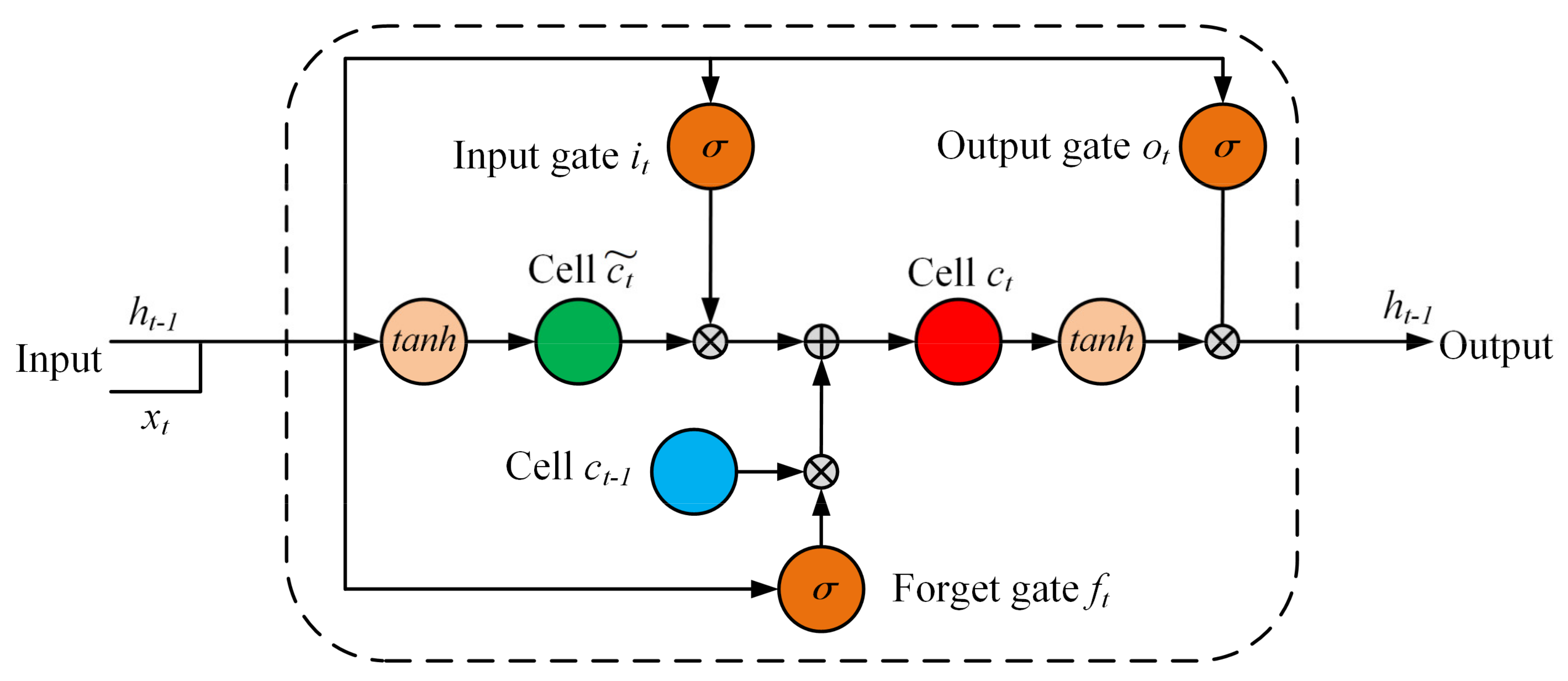
2.5.1. The Long Short-Term Memory (LSTM) Network

LSTM [28] is a recursive neural network, which is composed of several LSTM units. One LSTM unit includes three gate structures, as shown in Figure 6, namely, input gate, forgetting gate and output gate. These three gate structures are connected by memory cell units to realize purposeful selection of features in the network. The calculation formula of each module of LSTM unit type are as follows:
i t = σ W i × h t 1 , x t + b i
f t = o t W f × h t 1 , x t + b f
c ˜ t = t a n h W c × h t 1 , x t + b c
o t = σ W o × h t 1 , x t + b o
c t = f t c t 1 + i t c ˜ t
h t = o t t a n h c t
where [ ] represents vector connection, × represents matrix dot product, represents Hadamard product, σ represents sigmoid activation function, and t a n h represents hyperbolic tangent activation function. W i , W f , W c , W o are weight matrix and b i , b f , b c , b o indicate bias matrix. The weight matrix and bias matrix can be learned during the training process. x t represents the input of the network at time t, c ˜ t represents the updated value of memory cell state at time t. h t represents the state of the hidden layer at the time t. i t determines how much information in c ˜ t is used to update c t . f t determines how much information is retained in the memory cell unit at time t−1. The state of the hidden layer at time t is determined by h t , o t and c t .

2.5.2. LSTM Based on Multiple-Attention Modules (MA-LSTM) Proposed in This Paper

When the traditional LSTM model is used to model TEC data, the prediction weights of the data at any position in the historical sequence to the future data are equal, so it is impossible to adaptively and accurately model TEC. To solve this problem, this paper adds three attention modules [29], which can adaptively assign weights to each input sequence, so that the model can selectively focus on the historical sequence and reduce the prediction error. The proposed MA-LSTM TEC prediction model is shown in Figure 7.
The proposed MA-LSTM model includes four parts: the input layer, the LSTM layer, the multiple-attention layer and the output layer.
Input layer: Each sample includes two parts: feature vector x n and regression value y n (i.e., prediction value), which form an input sample in pairs as x n , y n .
LSTM Layer: This layer includes two independent LSTM neuron layers, one of which is provided with an L1 constraint and the other is not. These two layers, respectively, receives a pair of feature and regression value samples of the input layer x n , y n and process them separately. The processed results are spliced by concatenation function and transmitted to the next layer. The calculation formula of this layer is as follows:
k n = L S T M x n , y n
m n = L S T M x n , y n
r n = c o n c a t k n , m n
where k n represents the output of the first LSTM layer with an L1 constraint. m n represents the output of the unconstrained LSTM layer. r n represents the vector after connecting k n and m n . All r n are connected to form the output of this layer, which is h n .
Multiple-attention layer: This layer contains three parallel attention branches, which, respectively, receive the data from the LSTM layer. After receiving the data transmitted from the LSTM layer, each branch first calculates the similarity between each feature in the received data and the regression value through the attention function, and each feature obtains an attention score. The calculation formula of attention function selected in this paper is as follows:
s c o r e h n , y n = V T t a n h W h n + U y n
where W , V , U are the parameters that can be learned in the training process. After obtaining the attention score, then normalize it with the softmax function to obtain the probability distribution of attention. The specific calculation formula is as follows:
a 1 n = s o f t m a x s c o r e h n , y n
a 2 n = s o f t m a x s c o r e h n , y n
a 3 n = s o f t m a x s c o r e h n , y n
a 1 n , a 2 n , a 3 n represents the respective attention distribution values of the three branches. The softmax function is as follows:
S o f t m a x s c o r e h i , y i = e s c o r e h i , y i n = 1 n e s c o r e h n , y n
Then, a 1 n , a 2 n , a 3 n are, respectively, multiplied h n to obtain the output value of each attention branch. The calculation formula is as follows:
t 1 n = a 1 n × h n
t 2 n = a 2 n × h n
t 3 n = a 3 n × h n
Finally, connect the attention values of the three branches as the output of the attention layer.
Output layer: This layer includes a flattened layer and a fully connected layer. It is used to map the previously results into predicted values and then output them.

3. Experimental Results and Discussion

3.1. Model Parameter Selection

When MA-LSTM is used for TEC modeling, the optimal parameters of the model need to be determined first. In this paper, the grid search method is adopted to find the optimal super parameters. Result of grid search is as shown in Table 2.

3.2. Prediction Comparison of Different Stations

This paper first discusses the situation of TEC prediction at the second hour. The MA-LSTM model proposed in this paper is compared with the classical time series models LSTM, GRU and Att-BiGRU (in terms of structure, the LSTM is a three-layer gate structure, the GRU is a two-layer gate structure, and the Att-BiGRU is a two-layer gate structure in both directions). In the selected eight regions, samples were made according to the method described in Section 2.2. A total of 90% of the samples were used for training models and 10% for testing. The training data are 42715 TEC observations from 0:00 on 1 January 2002 to 18:00 on 30 December 2010, and the test data are 4747 TEC observations from 20:00 on 30 December 2010 to 24:00 on 31 December 2011. The predictive performance of each model is shown in Figure 8. The specific values are shown in Table 3.
As can be seen from Figure 8 and Table 3, the performance of the models with attention mechanism (MA-LSTM and Att-BiGRU) is significantly better than those of the models without attention mechanism (LSTM and GRU). The multiple-attention mechanism model proposed in this paper (MA-LSTM) is superior to the single attention mechanism model (Att-BiGRU). In the eight selected regions, the average RMSE of the MA-LSTM model proposed in this paper is 1.171TECU, which is reduced by 253.29, 228.44 and 35.01%, respectively, compared with LSTM, GRU and Att-BiGRU. The average R-square is 0.988, increased by 15.29, 13.04 and 0.01%, respectively. The average MAPE of our model is 0.054, which is increased by 248.15, 231.48 and 85.19%, respectively.

3.3. Prediction Comparison of Different Months

This section mainly discusses the prediction performance of the LSTM, GRU, Att BiGRU and MA-LSTM models in different months of the eight regions in Table 1. The training data are 42715 TEC sequences from 0:00 on 1 January 2002 to 18:00 on 30 December 2010, and the test data are TEC sequences from 12 different months in 2011. The mean prediction performance of different models in different months are shown in Table 4 and Figure 9. It can be seen that the fitting index R-square of our model exceeded 0.99 in July, August and September, and the maximum reaches 0.993, which appears in August. The lowest and highest RMSE values of our model are 1.086TECU and 1.267TECU, which are lower than those of the comparison models. The minimum MAPE of a single month of our model is 0.042, and the maximum is 0.071, which are significantly lower than those of the comparison model. That is to say, in all selected regions, in all months, in all comparison indicators, our MA-LSTM mode outperforms other comparison models. From Figure 9 we also can see that the R-square of our model is high in July, August and September, which indicates that the predicted value has a good fit with the real value in these three months. In March, April and May, the R-square is slightly low, and the prediction performance of the model is slightly poor, but even at the worst time, the fitting degree between the predicted value and the real value still reaches 0.965.

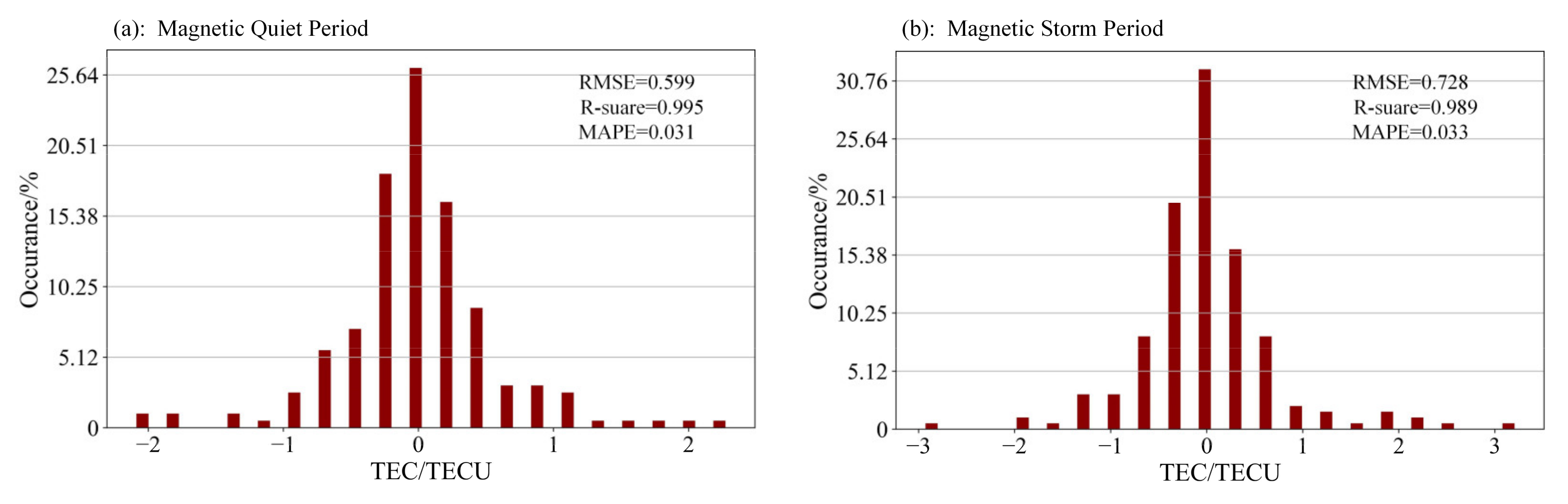
3.4. Prediction Comparison of Different Geomagnetic Conditions

In order to further study the prediction ability of the MA-LSTM model under different geomagnetic activities, we divided the test data into a magnetic quiet period and a magnetic storm period for comparative analysis (in this paper, samples with Kp < 3 are taken as magnetic quiet days, and samples with Kp > 3 and 100 < Dst 50 are taken as magnetic storm periods). Histograms of absolute error distribution during magnetic quiet periods and magnetic storm periods are shown in Figure 10, from which we can see that during the magnetic quiet period, the absolute error distribution of the prediction is more concentrated, basically between [−2,2], while during the magnetic storm, the absolute error distribution of the model is wider, reaching [−3,3], that is, the prediction effect of the MA-LSTM model during the magnetic quiet period is better than that during the magnetic storm. However, even during the magnetic storm period, the R-square of our model can still reach 0.989 in the selected area.
Figure 11 shows the comparison between the predicted value and the true value of a magnetic quiet day and a magnetic storm day, from which we can see that on the magnetostatic day, the predicted value matches the real value perfectly, while on a magnetic storm day, the error between the predicted value and the true value is relatively large, and the fitting is not very good.

4. Conclusions

In this paper, we proposed a multiple-attention LSTM (MA-LSTM)-based TEC prediction model, and applied it to the TEC prediction of eight locations—Beijing, Guangzhou, Harbin, Tibet, Yushu, Ziyang, Hangzhou and Heze in China. We compared our model in this paper with LSTM, GRU and Att-BiGRU. The experimental results show that the MA-LSTM model in this paper is obviously superior to the comparison models. We also discussed the prediction performance of our model in different month. Results show that our MA-LSTM model has the highest prediction performance in July, August and September, with the R-square reaching above 0.99. In March, April and May, the prediction performance is slightly poor, but even at the worst time, the R-square still reaches 0.965. We further discussed the prediction effect during a magnetic quiet period and a magnetic storm period. The results show that the prediction effect of a magnetic quiet period is slightly better than that of magnetic storm.
The author will study the grid prediction of TEC at multiple time points in the future.

Author Contributions

Writing—review and editing, H.L.; writing—original draft and methodology, D.L.; validation and resources, J.Y.; data curation, G.Y.; investigation, C.C.; software, Y.W.; project administration, W.X. All authors have read and agreed to the published version of the manuscript.

Funding

This research was supported by the Self funded scientific research and development program of Langfang Science and Technology Bureau, China (2022011046).

Institutional Review Board Statement

Not applicable.

Informed Consent Statement

Not applicable.

Data Availability Statement

Publicly available datasets were analyzed in this study. Ionospheric TEC data can be found here: https://pan.baidu.com/s/1yoJZd9MKWc_COcbK5Xk_XA, accessed on 27 August 2022.

Acknowledgments

Thanks to the TEC data provided by the European orbital determination Center (CODE), Thank Le Huijun of the Chinese Academy of Sciences for his help and suggestions.

Conflicts of Interest

The authors declare no conflict of interest.

References

  1. Kaselimi, M.; Voulodimos, A.; Doulamis, N.; Doulamis, A.; Delikaraoglou, D. A causal long short-term memory sequence to sequence model for TEC prediction using GNSS observations. Remote Sens. 2020, 12, 1354. [Google Scholar] [CrossRef]
  2. Tang, J.; Li, Y.; Yang, D.; Ding, M. An Approach for Predicting Global Ionospheric TEC Using Machine Learning. Remote Sens. 2022, 14, 1585. [Google Scholar] [CrossRef]
  3. Xiong, P.; Zhai, D.; Long, C.; Zhou, H.; Zhang, X.; Shen, X. Long short-term memory neural network for ionospheric total electron content forecasting over China. Space Weather 2021, 19, e2020SW002706. [Google Scholar] [CrossRef]
  4. Sharma, G.; Mohanty, S.; Kannaujiya, S. Ionospheric TEC modelling for earthquakes precursors from GNSS data. Quat. Int. 2017, 462, 65–74. [Google Scholar] [CrossRef]
  5. Belehaki, A.; Stanislawska, I.; Lilensten, J. An overview of ionosphere—Thermosphere models available for space weather purposes. Space Sci. Rev. 2009, 147, 271–313. [Google Scholar] [CrossRef]
  6. Samardjiev, T.; Bradley, P.A.; Cander, L.R.; Dick, M.I. Ionospheric mapping computer contouring techniques. Electron. Lett. 1993, 29, 1794–1795. [Google Scholar] [CrossRef]
  7. Tang, J.; Zhang, S.; Huo, X.; Wu, X. Ionospheric Assimilation of GNSS TEC into IRI Model Using a Local Ensemble Kalman Filter. Remote Sens. 2022, 14, 3267. [Google Scholar] [CrossRef]
  8. Qiao, J.; Liu, Y.; Fan, Z.; Tang, Q.; Li, X.; Zhang, F.; Song, Y.; He, F.; Zhou, C.; Qing, H.; et al. Ionospheric TEC data assimilation based on Gauss–Markov Kalman filter. Adv. Space Res. 2021, 68, 4189–4204. [Google Scholar] [CrossRef]
  9. Yue, X.A.; Wan, W.X.; Liu, L.B.; Le, H.J.; Chen, Y.D.; Yu, T. Development of a middle and low latitude theoretical ionospheric model and an observation system data assimilation experiment. Chin. Sci. Bull. 2008, 53, 94–101. [Google Scholar] [CrossRef]
  10. Akhoondzadeh, M. A MLP neural network as an investigator of TEC time series to detect seismo-ionospheric anomalies. Adv. Space Res. 2013, 51, 2048–2057. [Google Scholar] [CrossRef]
  11. Unnikrishnan, K.; Haridas, S.; Choudhary, R.K.; Dinil Bose, P. Neural Network Model for the prediction of TEC variabilities over Indian equatorial sector. Indian J. Sci. Res. 2018, 18, 56–58. [Google Scholar]
  12. Watthanasangmechai, K.; Supnithi, P.; Lerkvaranyu, S.; Tsugawa, T.; Nagatsuma, T.; Maruyama, T. TEC prediction with neural network for equatorial latitude station in Thailand. Earth Planets Space 2012, 64, 473–483. [Google Scholar] [CrossRef] [Green Version]
  13. Inyurt, S.; Sekertekin, A. Modeling and predicting seasonal ionospheric variations in Turkey using artificial neural network (ANN). Astrophys. Space Sci. 2019, 364, 62. [Google Scholar] [CrossRef]
  14. Huang, Z.; Yuan, H. Ionospheric single-station TEC short-term forecast using RBF neural network. Radio Sci. 2014, 49, 283–292. [Google Scholar] [CrossRef]
  15. Habarulema, J.B.; McKinnell, L.A.; Cilliers, P.J. Prediction of global positioning system total electron content using neural networks over South Africa. J. Atmos. Sol.-Terr. Phys. 2007, 69, 1842–1850. [Google Scholar] [CrossRef]
  16. Ruwali, A.; Kumar, A.J.S.; Prakash, K.B.; Sivavaraprasad, G.; Ratnam, D.V. Implementation of hybrid deep learning model (LSTM-CNN) for ionospheric TEC forecasting using GPS data. IEEE Geosci. Remote Sens. Lett. 2020, 18, 1004–1008. [Google Scholar] [CrossRef]
  17. Yuan, T.; Chen, Y.; Liu, S.; Gong, J. Prediction model for ionospheric total electron content based on deep learning recurrent neural networkormalsize. Chin. J. Space Sci. 2018, 38, 48–57. [Google Scholar] [CrossRef]
  18. Tang, R.; Zeng, F.; Chen, Z.; Wang, J.-S.; Huang, C.-M.; Wu, Z. The comparison of predicting storm-time ionospheric TEC by three methods: ARIMA, LSTM, and Seq2Seq. Atmosphere 2020, 11, 316. [Google Scholar] [CrossRef] [Green Version]
  19. Chimsuwan, P.; Supnithi, P.; Phakphisut, W.; Myint, L.M.M. Construction of LSTM model for total electron content (TEC) prediction in Thailand. In Proceedings of the 2021 18th International Conference on Electrical Engineering/Electronics, Computer, Telecommunications and Information Technology (ECTI-CON), Chiang Mai, Thailand, 19–22 May 2021; pp. 276–279. [Google Scholar]
  20. Ren, Q.; Li, M.; Li, H.; Shen, Y. A novel deep learning prediction model for concrete dam displacements using interpretable mixed attention mechanism. Adv. Eng. Inform. 2021, 50, 101407. [Google Scholar] [CrossRef]
  21. Li, X.; Yuan, A.; Lu, X. Vision-to-language tasks based on attributes and attention mechanism. IEEE Trans. Cybern. 2019, 51, 913–926. [Google Scholar] [CrossRef] [Green Version]
  22. Liu, F.; Zhou, X.; Cao, J.; Wang, Z.; Wang, T.; Wang, H.; Zhang, Y. Anomaly detection in quasi-periodic time series based on automatic data segmentation and attentional LSTM-CNN. IEEE Trans. Knowl. Data Eng. 2020, 34, 2626–2640. [Google Scholar] [CrossRef]
  23. Liu, L.; Zou, S.; Yao, Y.; Wang, Z. Forecasting global ionospheric TEC using deep learning approach. Space Weather 2020, 18, e2020SW002501. [Google Scholar] [CrossRef]
  24. Iluore, K.; Lu, J. Long short-term memory and gated recurrent neural networks to predict the ionospheric vertical total electron content. Adv. Space Res. 2022, 70, 652–665. [Google Scholar] [CrossRef]
  25. Lei, D.; Liu, H.; Le, H.; Huang, J.; Yuan, J.; Li, L.; Wang, Y. Ionospheric TEC Prediction Base on Attentional BiGRU. Atmosphere 2022, 13, 1039. [Google Scholar] [CrossRef]
  26. Li, Z.; Wang, N.; Liu, A.; Yuan, Y.; Wang, L.; Hernández-Pajares, M.; Krankowski, A.; Yuan, H. Status of CAS global ionospheric maps after the maximum of solar cycle 24. Satell. Navig. 2021, 2, 19. [Google Scholar] [CrossRef]
  27. Li, Z.; Wang, N.; Hernández-Pajares, M.; Yuan, Y.; Krankowski, A.; Liu, A.; Zha, J.; García-Rigo, A.; Roma-Dollase, D.; Yang, H.; et al. IGS real-time service for global ionospheric total electron content modeling. J. Geod. 2020, 94, 32. [Google Scholar] [CrossRef]
  28. Graves, A. Supervised sequence labelling. In Supervised Sequence Labelling with Recurrent Neural Networks; Springer: Berlin/Heidelberg, Germany, 2012; pp. 37–45. [Google Scholar]
  29. Galassi, A.; Lippi, M.; Torroni, P. Attention in natural language processing. IEEE Trans. Neural Netw. Learn. Syst. 2020, 32, 4291–4308. [Google Scholar] [CrossRef]
Figure 1. The information on the location of the eight regions on the map.
Atmosphere 13 01939 g001
Figure 2. TEC data of eight regions selected in this paper.
Atmosphere 13 01939 g002
Figure 3. TEC values after first-order difference.
Atmosphere 13 01939 g003
Figure 4. Schematic diagram of sample making process.
Atmosphere 13 01939 g004
Figure 5. The entire experimental process.
Atmosphere 13 01939 g005
Figure 6. Structure of an LSTM unit.
Atmosphere 13 01939 g006
Figure 7. MA-LSTM model structure for TEC prediction.
Atmosphere 13 01939 g007
Figure 8. Comparison of (a) RMSE, (b) R-square, (c) MAPE values of different models in all regions.
Atmosphere 13 01939 g008
Figure 9. Comparison of (a) RMSE, (b) R-square, and (c) MAPE values for various models in different months.
Atmosphere 13 01939 g009
Figure 10. Histograms of absolute error distribution during (a) magnetic quiet periods and (b) magnetic storm periods.
Atmosphere 13 01939 g010
Figure 11. Comparison of the predictive performance of a (a) magnetic quiet day and a (b) magnetic storm day.
Atmosphere 13 01939 g011
Table 1. The coordinates of the research areas in this paper.
RegionLatLon
Beijing40° N115° E
Guangzhou22.5° N115° E
Harbin45° N125° E
Tibet30° N90° E
Yushu35° N95° E
Ziyang30° N105° E
Hangzhou30° N120° E
Heze35° N115° E
Table 2. Optimal parameters of the MA-LSTM model gained by grid search.
Parameter NameOptimal Value
input_dim13
optimizerAdagrad
loss“RMSE” and ”R-Square”
activation“Relu”and “Softmax”
activity_regularizerL1(0.01)
learning rate0.01
batch_size64
num of hidden units64
Table 3. Comparison of prediction performance of different models.
AlgorithmIndicatorMeanBeijingGuangzhouHarbinTibetYushuZiyangHangzhouHeze
LSTMRMSE
(TECU)
4.1372.9624.6836.8342.7453.8804.5614.2253.208
GRU3.8463.2214.6136.6762.6833.0314.3923.4872.664
Att-BiGRU1.5810.8011.8674.2440.6500.9571.3541.4451.331
MA-LSTM1.1710.7181.5503.3770.6020.9341.2830.5430.358
LSTMR-square0.8570.8600.8560.8740.8770.8310.8500.8500.855
GRU0.8740.8390.8600.8800.8800.8900.8590.8930.895
Att-BiGRU0.9790.9880.9740.9530.9920.9870.9850.9800.972
MA-LSTM0.9880.9910.9820.9700.9930.9880.9860.9970.998
LSTMMAPE0.1880.1530.2170.2680.1490.1830.2050.1840.150
GRU0.1790.1660.2140.2670.1530.1430.2000.1540.135
Att-BiGRU0.1000.1390.1910.1660.0470.0510.0650.0690.072
MA-LSTM0.0540.0370.0750.1360.0340.0470.0610.0240.018
Table 4. Comparison of prediction performance by month.
AlgorithmIndicatorJanuaryFebruaryMarchAprilMayJuneJulyAugustSeptemberOctoberNovemberDecember
LSTMRMSE
(TECU)
4.1504.3573.9153.9643.8484.0724.1324.1684.2223.9504.3214.479
GRU3.8484.0063.6753.7033.5893.8183.8663.9173.9073.6643.9984.118
Att-BiGRU1.5331.6661.5521.5221.4311.6251.5341.5681.6131.5811.6451.664
MA-LSTM1.2021.1151.1841.1221.0861.2061.1451.1951.2021.1501.1541.267
LSTMR-square0.8540.6780.6180.5420.6230.7530.8710.9220.8710.7040.6570.798
GRU0.8740.7300.6650.6030.6780.7860.8890.9310.8900.7490.7080.829
Att-BiGRU0.9830.9590.9440.9370.9540.9650.9840.9890.9830.9590.9570.977
MA-LSTM0.9890.9810.9670.9650.9730.9810.9910.9930.9910.9780.9790.986
LSTMMAPE0.1680.1870.1610.1850.1890.1840.1480.1610.1850.2440.2630.189
GRU0.1580.1760.1560.1780.1770.1770.1410.1520.1710.2310.2480.177
Att-BiGRU0.0640.0720.0690.0790.0760.0750.0610.0650.0720.1010.1080.074
MA-LSTM0.0450.0490.0520.0560.0530.0530.0420.0480.0540.0710.0710.053
Publisher’s Note: MDPI stays neutral with regard to jurisdictional claims in published maps and institutional affiliations.

