
Atmosphere Critical Processes Sensing with ACP


1
Quantectum AG, Churerstrasse, 80, 8008 Pfäffikon, Switzerland
2
Space Research Institute RAS, Profsoyuznaya Str. 84/32, 117997 Moscow, Russia
*
Author to whom correspondence should be addressed.
Atmosphere 2022, 13(11), 1920; https://doi.org/10.3390/atmos13111920
Submission received: 8 October 2022
/
Revised: 12 November 2022
/
Accepted: 14 November 2022
/
Published: 18 November 2022
(This article belongs to the Section Meteorology)
Abstract
:This manuscript intends to demonstrate the diagnostic value of the previously discussed integrated parameter called atmospheric chemical potential (ACP) for tracking the atmospheric anomalies before strong earthquakes generated by the chain of processes initiated by air ionization due to radon emanation from the Earth’s crust. For this purpose, we considered several kinds of critical processes in the atmosphere using the ACP as an indicator and diagnostic tool: hurricane dynamics, the effects of radioactive pollution (the Chernobyl NPP accident), volcano eruptions and pre-earthquake atmospheric anomalies. We established that in all cases, some unusual features of the studied critical processes were revealed to be invisible when using certain methods of monitoring. This means that the application of ACP may improve the operative monitoring of the critical processes in atmosphere. In the cases of volcano eruptions and earthquakes, ACP can be used for short-term forecast.
1. Introduction
The atmosphere is one of the most unstable geophysical shells of our environment. This is connected with the fact that it contains water in three phase states simultaneously: liquid water (water drops), water vapor and ice crystals within clouds. The latent heat fluxes created (or absorbed) during the abrupt phase transitions of water in atmosphere can be monitored with the help of the integrated parameter, calculated using the meanings of air temperature and relative humidity, called the atmospheric chemical potential (ACP) [1,2]. This concept appeared while considering the processes of air ionization by different sources: galactic cosmic rays in upper atmosphere, thunderstorm discharges in troposphere and radon emanating from the Earth’s crust in the near-ground layer of the atmosphere. Nuclear accidents, such as Chernobyl in 1986 or Fukushima in 2011, and other sources of radioactive pollution can also provide air ionization. Regardless of the source of ionization, newly formed ions play the role of the center of nucleation for water vapor present in the atmosphere. For example, the ions produced by galactic cosmic rays are largely responsible for the cloud’s formation [3]. The process of water molecules attachment to ions is known as the ion’s hydration, which, in the sense of the phase state of the water molecules, is equivalent to condensation, when after molecule attachment to the ion, the latent heat of condensation is released. In direct laboratory experiments with corona discharge, it was established, using mass-spectrometer measurements, that several hundred water molecules can be attached to the ionized gas molecule [4]. This process is called ion-induced nucleation (IIN) and has an avalanche character [5]. The most important thing that was established by [6] is the bond energy of a water molecule and ion is larger than the bond energy of water molecules in the water drop. The difference between these bond energies is the atmospheric chemical potential. Why do we call it the chemical potential? Because at the moment of water molecule condensation/evaporation or attachment/detachment to the ion, the latent heat release/absorption is equal to the chemical potential. However, due to the fact that it is also equal to the latent heat, the chemical potential can be expressed using the thermodynamic parameters, namely the air temperature and relative humidity [1]:
where Tg is the air temperature and H is relative humidity.
ACP = 5.8 × 10⁻¹⁰ (20Tg + 5463)2ln(100/H).
Systems that are far from thermodynamic equilibrium can not only energy exchange with the environment but also the mass of matter. Such systems, in contrast to closed ones, are called open. The energy in them can be dissipated and irreversibly transferred to other types of energy, for example, into the energy of the vibrational or thermal motion of atoms. Therefore, such systems are called dissipative. At present, a large number of non-equilibrium physical processes are known, in which self-organization effects arise, leading to the formation of structures ordered in space and time [7]. The atmosphere is an ideal object that fits this definition. In case of hurricane formation, the thermal energy of the ocean water is transformed into the air mass movement as a convection [8]. The self-organization process starts with vertical convection movement and spiral movement formed by air mass moving to the center of depression [9,10]. Its horizontal movement is transformed into a spiral due to the Earth’s rotation. The hurricane machine starts spinning with continuous heat exchange in water evaporation in lower layers and condensation at the top of the hurricane with continuous latent heat release and absorption [11]. The thunderstorm activity inside the hurricane [12] increases the heat and mass exchange through ionization. It should be underlined that the question of hurricane formation still remains unresolved, and new data provided by ACP may help achieve a more profound understanding of hurricane birth and dynamics.
The air ionization provided by natural and artificial radioactivity essentially violates the thermodynamic equilibrium of the boundary layer of the atmosphere providing the enormous number of nucleation centers and the consequent additional latent heat release [2]. Taking into account that these effects have a spontaneous, not regular character, they cannot be predicted by the regular weather forecast, while the ACP can be used not only to monitor these phenomena but also to predict them, because in case of earthquakes and volcano eruption they appear a few days/hours before the event itself [1].
The intention of the present paper is to demonstrate the diagnostic value of ACP. We will consider the atmospheric characteristics of the category 4 Hurricane Sam in September–October 2021 during its pass over the whole Atlantic Ocean from West Africa to the vicinity of Greenland. Then the ability of ACP to detect the consequences of atomic reactor explosion during the Chernobyl catastrophe in April–May 1986 will be tested in order to demonstrate its impact on the atmospheric parameters. The two last sections will be devoted to the ACP monitoring of volcano eruptions and earthquakes, including the ability of this parameter to be used as a short-term precursor. In all cases we produce the spatial distribution of ACP at the 250 m altitude, according to Formula (1) using the data of the global forward processing atmospheric model GEOS-FP provided by NASA Global Modeling and Assimilation Office (https://portal.nccs.nasa.gov/datashare/gmao/geos-fp/das/ (accessed on 21 April 2021)). For the Chernobyl incident we used the MERRA model from the same center.
2. Hurricane Sam Dynamics
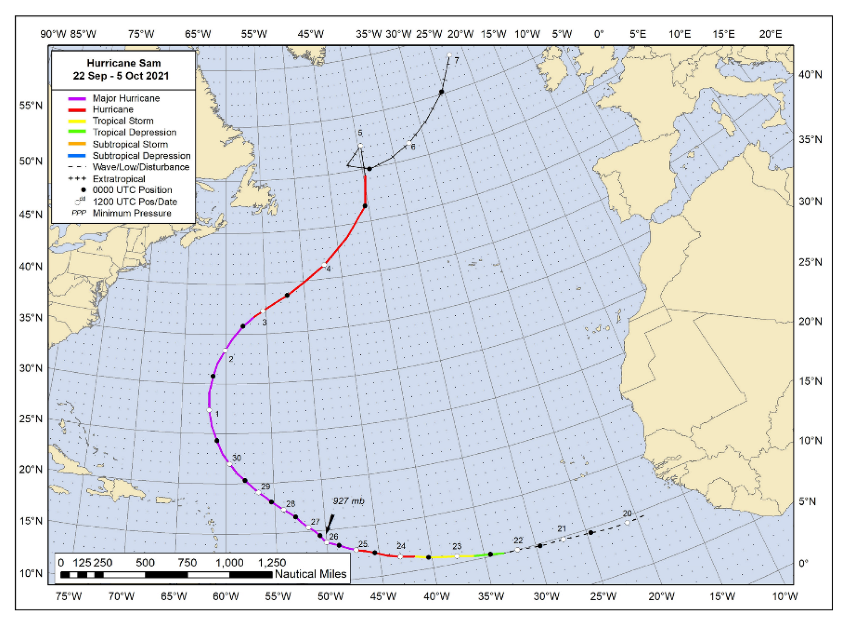
Hurricane Sam was a category 4 long-lived hurricane. Starting from the 22 September in the vicinity of Cabo Verde it ended its life south-west of Greenland on the 9 October. It was the fifth “longest lasting, most intense” Atlantic hurricane, as measured by accumulated cyclone energy, on record since 1966 [13]. The hurricane track, according to NOAA Ocean Prediction Center, is shown in Figure 1.
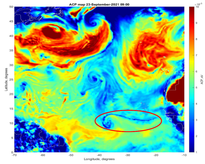
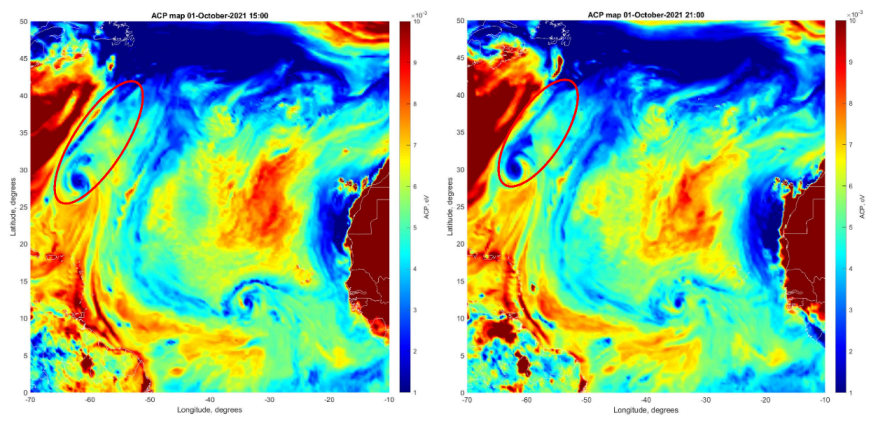
We want to demonstrate some interesting features of hurricane development which have either been ignored or cannot be detected by other methods. In Figure 2, the hurricane “feeding” from the remote area during the stage of its strengthening is demonstrated. On 23 September, when the depression started to form into the spiral shape, the very long (more than 2000 km) thin “tail”, almost reaching to the African shore, is chasing after it. We see a similar (but thicker) tail at the stage of hurricane decay on the 1 October. The elongated structure is formed from northern areas in direction of the hurricane position (Figure 3, left panel), and 6 h later it merges with the hurricane, thus forming the “tail”, feeding it from the wet air (Figure 3, right panel).
A lot of other interesting features regarding the hurricane dynamics were revealed with the help of ACP but this will be the subject of a separate paper. Here we only cover on two more phenomena regarding the hurricane structure and dynamics that were observed in the air temperature distributions, bearing in mind that air temperature is a component of ACP.
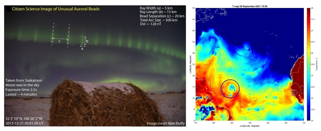
The first feature concerns the generation of the bead instability at the hurricane periphery during its recovery stage. During its pass through the Atlantic, Hurricane Sam twice lost its eye wall structure and then recovered it. Only in the period of the hurricane restructuring its bead-like structures were similarities to the bead instability sometimes developed in the auroral substorms observed [14]. In the left panel of Figure 4, the substorm bead instability is shown, while in the right panel the bead structure is observed in Hurricane Sam’s periphery.
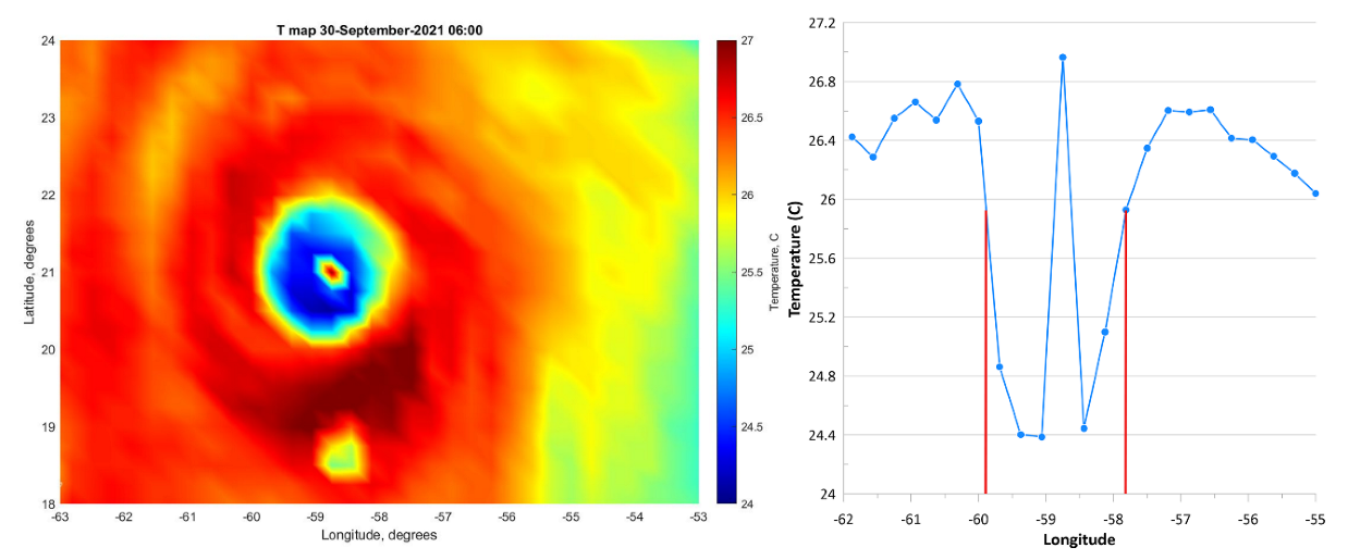
The second interesting feature is the formation of a fixed temperature ring separating the circle structure of the hurricane eye from its spiral structure at the stage of the well-developed hurricane. The temperature of the yellow circle is 25.9 °C, i.e., close to the temperature of the ocean surface, and its diameter is nearly 200 km (Figure 5).
From a physical point of view, the lower temperature in the internal part of hurricane is observed within the area of vertical upward convection, where the processes of evaporations prevail, which leads to the latent heat absorption. The red external part corresponds to the area of condensation and precipitation with the release of latent heat. The yellow border is a transition zone with zero balance of the absorbed and released latent heat. The red spot is within the clear eye of the hurricane where fair and calm weather conditions are maintained.
3. Nuclear Emergencies Monitoring with ACP
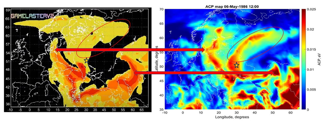
In this section, we would like to demonstrate the possibilities of ACP in monitoring the situation with the radioactive pollution of our environment. Regarding the sad history of nuclear emergencies, we can mention the Three-Mile Island (USA) accident on the 28 March 1979 [15], Chernobyl disaster (USSR) 26 April 1986 (International, 1986) and the Fukushima NPP disaster (Japan) 13–17 March 2011 [16]. Because the first and third accidents were on a small spatial scale encompassing only a few tens of km of essential pollution, we decided to consider the largest in scale: the Chernobyl event, with well-documented spatial distributions of radioactive clouds which propagated through the whole of Europe. Here we should keep in mind that the first blast of the reactor was very powerful and spread the radioactive matter over several km of altitude, while our model calculates the effects in the atmosphere at a 250 m altitude. This is why we do not see the explosion effect on the 26 of April. Starting from the 27 April, measures were being taken to stop the combustion of graphite. Materials were being dumped into the reactor from helicopters—sand and clay, lead, dolomite and boron compounds. The purpose of this “bombing” was to localize the burning of graphite in order to help reduce the neutron flux (to reliably “quench” the chain reaction and eliminate the prerequisites for its occurrence again) and to create a kind of bulk filter to reduce the release of aerosols. The backfilling of the collapse of the 4th reactor was carried out, among other things, in order to reduce the release of radioactive aerosols. Although at the same time, it so happened that the discharges from the helicopters of these materials, which began from the middle of the day on April 27, were a source of radioactive aerosols entering the atmospheric air. The cargo was carried on an external sling and unhooked at a height of about 200 m. It was impossible to fly lower because of the ventilation pipe, the cut of which was at a height of about 150 m and high exposure dose rates. Each landing of the cargo was accompanied by the appearance of a cloud of dust, i.e., aerosols. According to our model [1] the charged aerosols are the perfect centers for water-drop nucleation, and process of nucleation is followed by the latent heat release. It is only during this period that we see the maximum effect in our ACP maps. The spatial distribution of cesium-137 in air above the ground om 06 May 1986 is shown in the left panel of Figure 6 (https://www.irsn.fr/EN/publications/thematic-safety/chernobyl/Pages/The-Chernobyl-Plume.aspx (accessed on 10 October 2022)), while in the right panel we demonstrate the spatial distribution of ACP on the same day with a well-developed structure of several sleeves similar to the left figure.
Comparing the figures, we should mark the similarity of distributions. Cesium-137 distribution also was measured close to the ground surface. The obtained result is very firm confirmation that atmospheric parameters can be modified by radioactivity and create the thermal anomalies while the ACP can be used as a remote sensing instrument for radioactive pollution monitoring.
4. ACP Monitoring of Volcano Activity
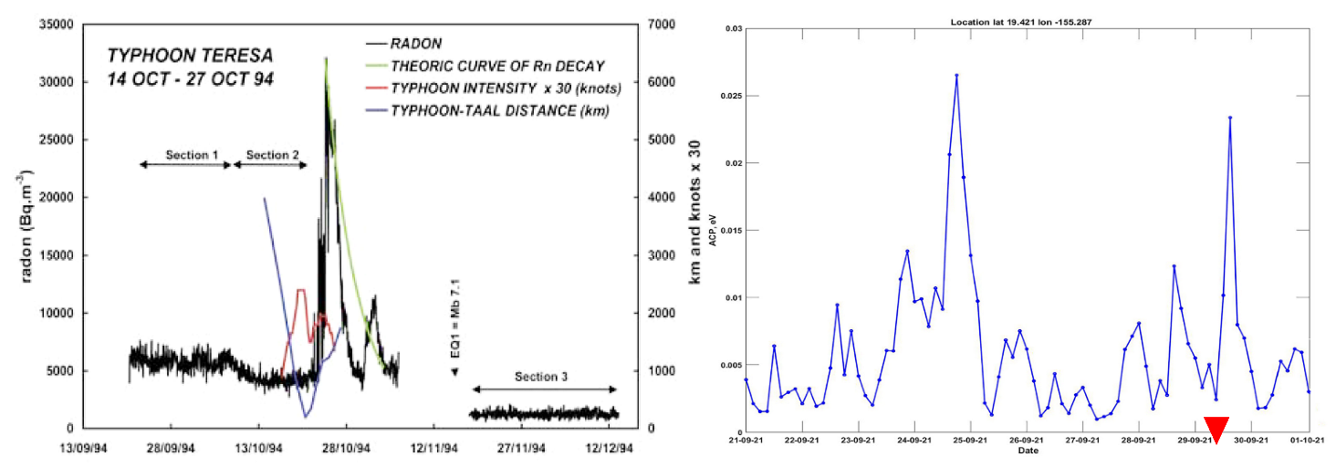
The ACP monitoring of volcano activity on the Kamchatka peninsula [17] has demonstrated that the sharp peaks of ACP registered over volcano caldera appear several days before the volcano eruption. They differ from the earthquake precursors simply by peak sharpness and reflect a sharp rise in radon volumetric activity, as it was registered during the approaching of the Teresa typhoon to the Taal volcano (Luzon island, Philippines) in November 1994 [18]. Radon was continuously monitored at the Taal volcano from June 1993 to November 1996.
In Figure 7, we compare the radon variation at the Taal volcano and ACP variation four days before the Kīlauea volcano on the island of Hawai’i on 29 September 2021.
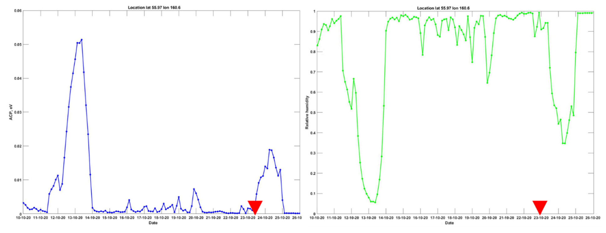
It should be mentioned that the relative humidity drops equally very sharp from nearly 100% to practically zero during the positive peak of ACP. We demonstrate this for the case of the Bezymyanny volcano eruption when a precursory peak was registered 10 days before the volcano eruption on 22 October 2020 (Figure 8).
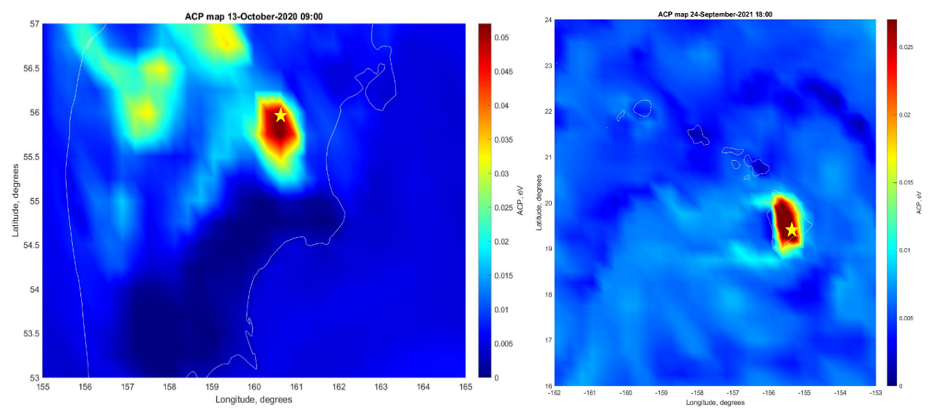
To be sure that the observed effect is really connected with volcano activity we need to build a spatial distribution of ACP over the volcano’s position. Figure 9 shows the ACP distribution over the volcano Bezymyanny (left panel) and volcano Kīlauea (right panel) at a time when the main maximum of ACP was observed.
When comparing both cases, we should note that the effect at Kamchatka is essentially stronger by nearly an order of magnitude, but the spatial size of the ACP anomaly is two times smaller than at Hawai’i. Of all the demonstrated properties of the ACP behavior, the most important is the effect that appears before the eruption, which can be used for the purposes of the short-term forecast of the volcano eruptions.
5. Air Pollution Monitoring
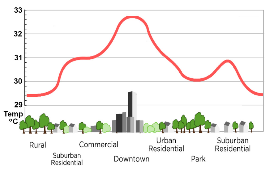
During the last few decades, a new term has appeared—the “urban heat islands” [19,20]. This term is applied to large cities usually with more than million citizens and with high energy consumption and a developed industry and transport structure. Each of these components emits a large amount of heat into the environment, which leads to the formation of an area over the city with elevated air temperatures (Figure 10).
According to [20], the thermal pollution in St. Petersburg is about 586 PJ per year. The main contribution to thermal pollution is provided by consumers of thermal energy (220 PJ per year), transport (220 PJ per year), consumers of electric energy (120 PJ per year) and the population (26 PJ per year). Of these sources, one stands apart—air pollution. Its thermal effect is not direct heat emission into atmosphere but latent heat release due to water vapor condensation on aerosols. Only ACP can monitor this part of the thermal anomaly, because the aerosols usually are charged, what intensifies the process of condensation and creates an excess of the thermal flux in comparison with the usual water condensation process. This excess is attributed to the ACP effect [2].
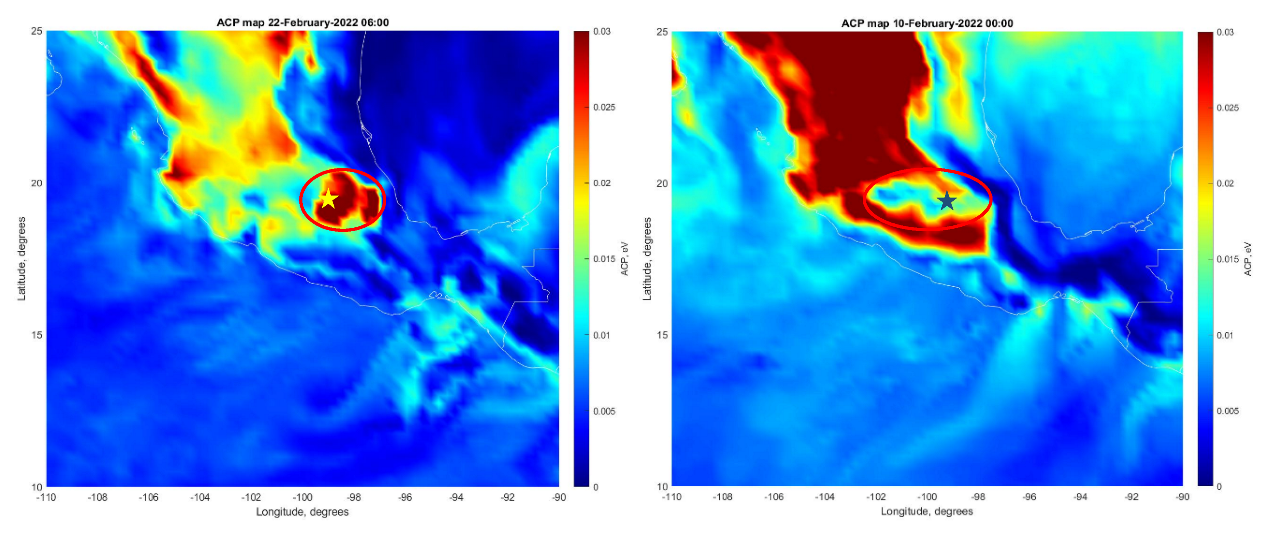
The real picture turned out to be different to what we expected. We observed both the increased values of ACP around the monitored city and lower values in comparison to surrounding space. Periods with no effect were also observed. This means that the problem needs the further investigation; nevertheless, the increased values of ACP over Mexico City and its surroundings (Figure 11, left panel) and the lower values of ACP over the monitored area (Figure 11, right panel) are demonstrated. The coordinates of the Mexico City are marked by the asterisks.
Of course, statistical studies in different seasons of the year are necessary, and other geographical areas should be investigated. Figure 11 is only a demonstration of possibilities which are provided by the ACP monitoring of air pollution.
6. ACP Monitoring of Seismic Activity
In reality, ACP was developed more than 10 years ago, and its main purpose was aimed to be a solution of the problem of short-term earthquake forecasting [6]. The huge amount of information concerning ACP application has been collected up to the present, and the main properties of the ACP in relation to the seismic process are demonstrated lower.
ACP anomalies are generated due to increased radon release during the last stage of the seismic cycle (few weeks/days before the main shock) [21].
The ionization of the near-ground layer of the atmosphere by radon initiates the thermodynamic instability with the latent heat release and the modification of the meteorological parameters (air temperature, relative humidity and air pressure) not considered by the meteorological forecast [22].
Because the ACP is a proxy of radon activity and its temporal variations are very similar to radon and after reaching the peak values (usually on a monthly time scale) the magnitude of ACP drops, and the time of this drop is very close to the moment of main shock.
Usually, the size of the ACP anomaly corresponds to the earthquake preparation zone [23]. It can be a linear-shaped anomaly or a single spot filling the preparation zone.
The ACP magnitude is weaker over the ocean. There are special areas with very weak ACP anomalies or with a reversed shape (negative variations).
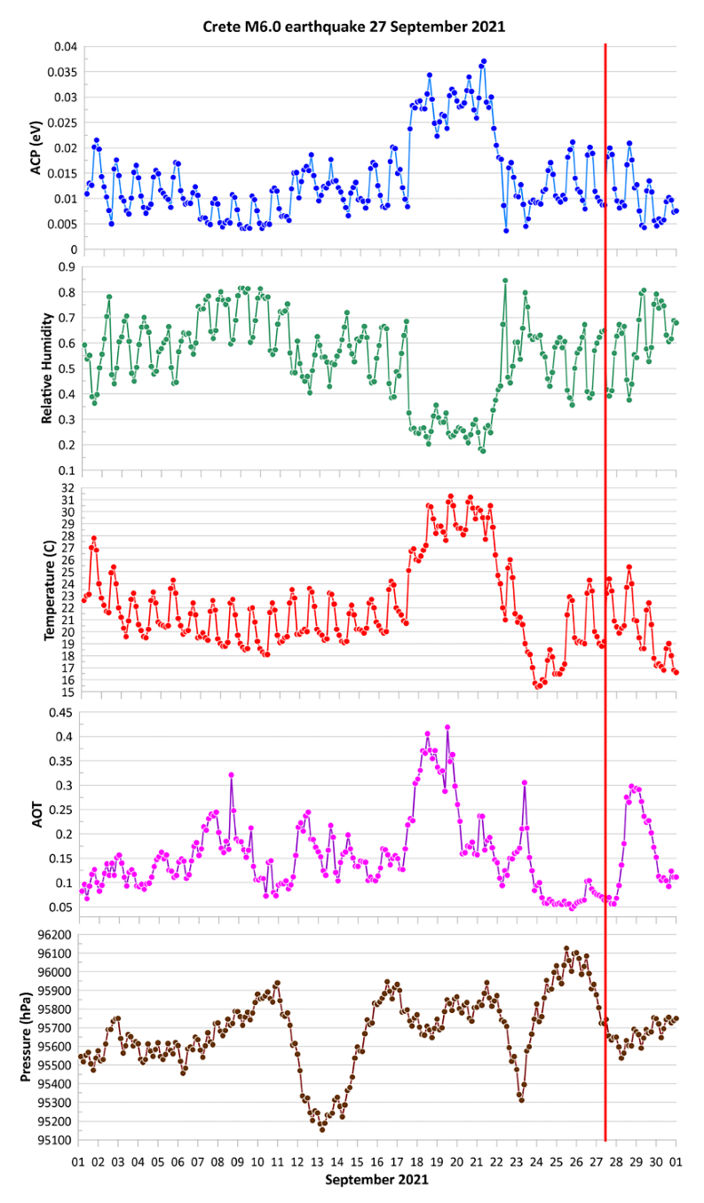
In Figure 12, the variations of ACP and meteorological parameters before the M6 earthquake on the island of Crete (Greece) on 27 September 2021 are demonstrated. We also included the aerosol optical thickness (AOT), which shows the formation of large ion clusters reaching the aerosol size.
It is necessary to provide comments regarding the air pressure variations. As we know, according to Dalton’s law, air pressure is equal to the sum of partial pressures of the gases composing the air, where water vapor is one of the components. From 16 to 22 September, we observed the strong decrease of the relative humidity (from 70% to 20%), which automatically lowers the water vapor partial pressure. On the air pressure graph, one can see the small air pressure drop from 16 to 22 September manifesting the drop of the water vapor partial pressure.
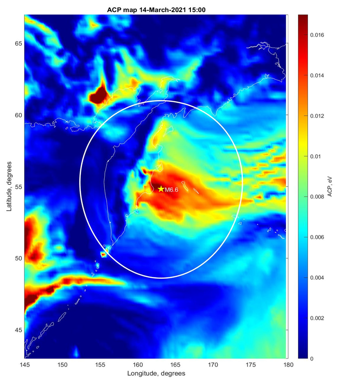
Another important feature of the ACP is its spatial distribution in relation to the earthquake epicenter position. In general, the ACP anomaly occupies the space within the earthquake preparation zone [23], which gives the opportunity to estimate the magnitude of the impended earthquake. Depending on the geological conditions (different level of radon activity, different earthquake focal mechanism, different climatic conditions, etc.) the shape of the anomaly may be different, but in majority of cases, the anomaly is within the preparation zone. The example of the ACP distribution two days before the M6.6 earthquake off the coast of Kamchatka on 16 March 2021 is presented in Figure 13.
One can see that the anomaly occupies nearly 2/3 of the earthquake preparation zone (white circle) and the most intensive amplitude is registered near the epicenter point marked by the star.
Taking into account that we are dealing with atmospheric phenomena, the anomaly is involved in atmospheric movement dragged by the wind.
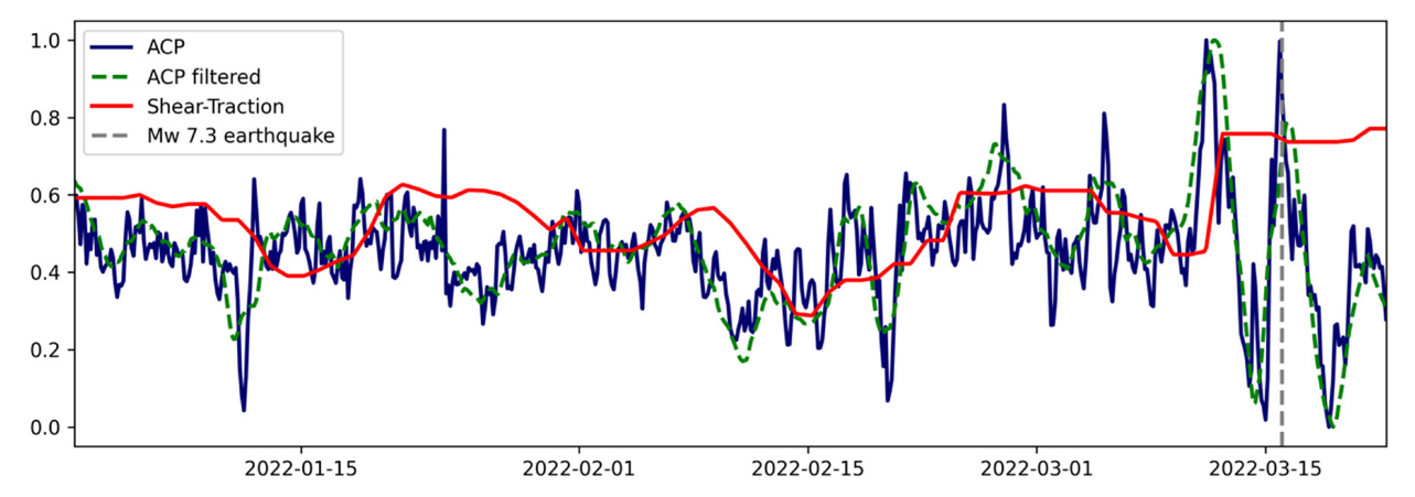
Most striking is the fact that ACP correlates with the variations of the shear-traction field in the Earth’s crust, which can be modeled in real time and forecasted [24]. This reflects the fact that crust deformations (expressed in the form of the shear-traction field) increase the radon release which, in turn, increases the magnitude of the chemical potential through the air ionization process. The example of the simultaneous registration of ACP and modeled shear-traction field around the time of the Fukushima M7.3 earthquake in Japan on 16 March 2022, is presented in the Figure 14.
One can see the synchronous sharp increase of the ACP (blue curve) and shear traction (red curve) 3 days before the Fukushima M7.3 earthquake. The combination of these two parameters manifest a clear physical effect of the earthquake preparation process, which, contrary to the probabilistic approach, may be used (in the case of reliable statistical confirmation) for short-term earthquake forecasting.
7. Discussion
The atmospheric chemical potential (ACP), initially utilized to monitor the precursory phenomena in the near-ground layer of the atmosphere, has been provisionally applied to other atmospheric phenomena in which air ionization takes place, or air contains the large number of charged particles. When used for nuclear accidents, such as Chernobyl, its use is evident, whereas in the case of hurricanes or air pollution it is not entirely clear. Let us consider the presented cases item by item.
- Hurricanes
It is known that hurricane activity is accompanied by thunderstorm activity [12] and thunderstorm discharges can produce air ionization. In addition, even without the thunderstorm activity, the electric fields inside the hurricane measured by the direct air flights through the hurricane reached values of >20 kV/m [25], which is more than enough to ionize the air molecules with the ionization potential of less than 20 eV. This means that the ACP conception is quite applicable to the processes inside the hurricane.
- 2.
- Radioactive pollution
This application of ACP is quite natural because it initially used as a source the natural radioactivity—radon emanation. The effects in atmosphere depend not only on the radioactive emission intensity but also on the source size. In this regard, during the Chernobyl disaster, the spread of radioactive substances had almost continental scale due to their reaching the high layers of the atmosphere. The thermal anomaly was registered not only in the lower atmosphere but also at the upper cloud boundary in the form of the long-wave infrared emission (OLR) [26]. But the strongest argument is that the ACP distribution measured at the 250 m altitude and shown in the Figure 6 in great extend repeats the distribution of radioactive Cesium-137 measured near ground surface
- 3.
- Volcanoes eruption
There is not very much literature on radon activity due to the crust deformation before volcano eruption, that’s why we used the result of direct radon measurements in the vicinity of Taal volcano showing the characteristic shape of the radon behavior caused by the deformation produced by pressure anomaly while approaching the typhoon Teresa (Figure 7, left panel). Taking into account that the ACP is a proxy of radon activity, we expected a similar shape of radon emanation before the volcano eruptions, which was perfectly confirmed by many experimental observations and demonstrated here in two cases of volcano eruptions in two completely different geographic zones: the Hawaiian islands (Figure 7, right panel) and the Kamchatka peninsula (Figure 8). The size of the ACP anomaly in both cases is demonstrated in Figure 9.
- 4.
- Air pollution
The most controversial and unexpected outcome was the case of air pollution. It is well known that heat islands exist over polluted megacities. We expected that the latent heat release by the ionized aerosols would be the main sources of these islands. The aerosols in air always have an electric charge due to ionization by galactic cosmic rays and to the attachment of the charged molecules of air gases. However, sometimes contrary to the formed heat island shown in the left panel of the Figure 1, we observe the brightening of the sky around a megacity (in our case, Mexico city). To this point we can only speculate that the aerosols have grown to the rain drop size and precipitated with the rain clearing the sky. This problem needs the further investigation and clarification, which will be done in future publications.
- 5.
- Seismic activity monitoring
8. Conclusions
We have demonstrated the possibility of monitoring the hidden parameters of the critical processes in the atmosphere initiated by the air ionization sources of different origin. The main result of the ionization and consequent atmospheric ion hydration is the latent heat release accompanied by the changes of air temperature and relative humidity. ACP is the measure of these variations and extend of the process criticality. It becomes most obvious when analyzing the ACP variations before earthquakes over the earthquake preparation zone.
It is necessary to say that air ionization is the intrinsic property of our environment, penetrating all geospheres. We did not examine this issue but one of the most important processes is the global cloud coverage formation due to air ionization by the galactic cosmic rays which are the main source of air ionization at over 1 km in altitude. At the lower atmosphere, the principal source of ionization is radon participating in the creation of air ions, providing column air conductivity in the global electric circuit.
Except the external sources of ionization, we should consider the internal processes of ionization, such as the electric charge separation in clouds, which leads to the formation of strong electric fields by an order of tens kV/m producing additional ionization and thunderstorm discharges.
The final issue to be considered is the air pollution by aerosols in industrial areas and mega-cities and the possible radioactive pollution as a result of accidents at nuclear power plants and nuclear tests.
In this way, we can apply ACP technology as a universal diagnostic tool able in addition to point ground-based measurements to provide a global picture of the large-scale processes in the atmosphere.
Author Contributions
Conceptualization, methodology, investigation S.P.; software, data processing, data curation P.B. All authors have read and agreed to the published version of the manuscript.
Funding
This research was funded by Quantectum AG.
Institutional Review Board Statement
Not applicable.
Informed Consent Statement
Not applicable.
Data Availability Statement
Not applicable.
Conflicts of Interest
The authors declare no conflict of interest.
References
- Pulinets, S.A.; Ouzounov, D.P.; Karelin, A.V.; Davidenko, D.V. Physical Bases of the Generation of Short-Term Earthquake Precursors: A Complex Model of Ionization-Induced Geophysical Processes in the Lithosphere–Atmosphere–Ionosphere–Magnetosphere System. Geomagn. Aeron. 2015, 55, 540–558. [Google Scholar] [CrossRef]
- Pulinets, S.; Ouzounov, D.; Karelin, A.; Boyarchuk, K. Earthquake Precursors in the Atmosphere and Ionosphere; Springer Nature: Berlin/Heidelberg, Germany, 2022; 312p. [Google Scholar] [CrossRef]
- Svensmark, H.; Pedersen, J.O.P.; Marsch, N.D.; Enghoff, M.B.; Uggerhøj, U.I. Experimental evidence for the role of ions in particle nucleation under atmospheric conditions. Proc. R. Soc. A 2007, 463, 385–396. [Google Scholar] [CrossRef]
- Sekimoto, K.; Takayama, M. Influence of needle voltage on the formation of negative core ions using atmospheric pressure corona discharge in air. Int. J. Mass Spectrom. 2007, 261, 38–44. [Google Scholar] [CrossRef]
- Anikin, G.V.; Vlasov, V.A. Comparison of theories of ion-induced nucleation. Russ. J. Phys. Chem. 2014, 88, 22–27. [Google Scholar] [CrossRef]
- Boyarchuk, K.A.; Karelin, A.V.; Nadolsky, A.V. Statistical analysis of the dependence of the correction of the chemical potential of water vapor in the atmosphere on the remoteness of the earthquake epicenter. Vopr. Elektromekhaniki 2010, 116, 39–45. [Google Scholar]
- Kadomtsev, B.B.; Ryazanov, A.N. What is synergy? Nature 1983, 8, 2–11. [Google Scholar]
- Huang, Q.; Ge, X.; Peng, M. Simulation of Rapid Intensification of Super Typhoon Lekima. Part I: Evolution Characteristics of Asymmetric Convection Under Upper-Level Vertical Wind Shear. Front. Earth Sci. 2021, 9, 739507. [Google Scholar] [CrossRef]
- Anthes, R.A. Hot Towers and Hurricanes: Early Observations, Theories, and Models. Meteorol. Monogr. 2003, 29, 139. [Google Scholar] [CrossRef]
- Smith, R. Hurricane Force. Phys. World 2006, 32–37. [Google Scholar] [CrossRef]
- Trenberth, K.E.; Davis, C.A.; Fasullo, J. Water and energy budgets of hurricanes: Case studies of Ivan and Katrina. J. Geophys. Res. 2007, 112, D23106. [Google Scholar] [CrossRef]
- Mikhailov, Y.M.; Druzhin, G.I.; Mikailova, G.A.; Kapustina, O.V. Thunderstorm activity dynamics during hurricanes. Geomagn. Aeron. 2006, 46, 783–795. [Google Scholar] [CrossRef]
- Pasch, R.J.; Roberts, D.P. Hurricane Sam, National Hurricane Center Tropical Cyclone Report, AL 182021; NOAA: Boulder, COP, USA, 2022. [Google Scholar]
- Derr, J.R. Stability Analyses of Auroral Substorm Onset and Solar Wind. Ph.D. Dissertation, The University of Texas at Austin, Austin, TX, USA, 2019. [Google Scholar]
- Rogovin, M.; Frampton, G.T., Jr. Three-Miles Island. A report to the Commission and to the Public; Nuclear Regulatory Commission Special Inquiry Group: Washington, DC, USA, 1980; 805p. [Google Scholar]
- Lipscy, P.; Kushida, K.; Incerti, T. The Fukushima Disaster and Japan’s Nuclear Plant Vulnerability in Comparative Perspective. Environ. Sci. Technol. 2013, 47, 6082–6088. [Google Scholar] [CrossRef] [PubMed]
- Pulinets, S.; Ouzounov, D.; Davidenko, D.; Petrukhin, A. Multiparameter monitoring of short-term earthquake precursors and its physical basis. Implementation in the Kamchatka region. E3S Web Conf. 2016, 11, 00019. [Google Scholar] [CrossRef] [Green Version]
- Richon, P.; Sabroux, J.C.; Halbwachs, M.; Vandemeulebrouck, J.; Poussielgue, N.; Tabbagh, J.; Punongbayan, R. Radon anomaly in the soil of Taal volcano, the Philippines: A likely precursor of the M 7.1 Mindoro earthquake. Geophys. Res. Lett. 1994, 30, 1482. [Google Scholar] [CrossRef]
- Li, Y.; Zhao, X. An empirical study of the impact of human activity on long-term temperature change in China: A perspective from energy consumption. J. Geophys. Res. 2012, 117, D17117. [Google Scholar] [CrossRef]
- Gorshkov, A.S.; Vatin, N.I.; Rymkevich, P.P. Climate change and the thermal island effect in the million-plus city. Environ. Sci. Eng. Constr. Unique Build. Struct. 2020, 89, 8902. [Google Scholar] [CrossRef]
- Pulinets, S.; Ouzounov, D.; Karelin, A.; Davidenko, D. Lithosphere–Atmosphere–Ionosphere–Magnetosphere Coupling—A Concept for Pre-Earthquake Signals Generation. In Pre-Earthquake Processes: A Multidisciplinary Approach to Earthquake Prediction Studies; Ouzounov, D., Pulinets, S., Hattori, K., Taylor, P., Eds.; AGU/Wiley: Washington, DC, USA, 2018; pp. 77–98. [Google Scholar] [CrossRef]
- Pulinets, S. Thermodynamic Instability of the Atmospheric Boundary Layer as a Precursor of an Earthquake. In Nonequilibrium Thermodynamics and Fluctuation Kinetics. Fundamental Theories of Physics; Brenig, L., Brilliantov, N., Tlidi, M., Eds.; Springer: Cham, Switzerland, 2022; Volume 208, pp. 313–323. [Google Scholar] [CrossRef]
- Dobrovolsky, I.P.; Zubkov, S.I.; Myachkin, V.I. Estimation of the size of earthquake preparation zones. Pure Appl. Geophys. 1979, 117, 1025–1444. [Google Scholar] [CrossRef]
- Pulinets, S.; Vičič, B.; Budnikov, P.; Potočnik, M.; Dolenec, M.; Žalohar, J. Correlation between Shear-Traction field and Atmospheric Chemical Potential as a tool for earthquake forecasting. In Proceedings of the 3rd European Conference on Earthquake Engineering and Seismology, Bucharest, Romania, 4–9 September 2022. [Google Scholar]
- Black, R.A.; Hallet, J. Electrification of the Hurricane. J. Atmos. Sci. 2004, 56, 2004–2028. [Google Scholar] [CrossRef]
- Laverov, N.P.; Pulinets, S.A.; Ouzounov, D.P. Application of the Thermal Effect of the Atmosphere Ionization for Remote Diagnostics of the Radioactive Pollution of the Atmosphere. Dokl. Earth Sci. 2011, 441 Pt 1, 1560–1563. [Google Scholar] [CrossRef]
- Pulinets, S.; Ouzounov, D. The Possibility of Earthquake Forecasting. Learning from Nature; IOP Publishing: Bristol, UK, 2018; 167p, Available online: https://iopscience.iop.org/book/978-0-7503-1248-6 (accessed on 8 October 2022).
Figure 1.
Best track positions for Hurricane Sam, 22 September–5 October 2021. Tracking during the extratropical stage is partially based on analyses from the NOAA Ocean Prediction Center.
Figure 1.
Best track positions for Hurricane Sam, 22 September–5 October 2021. Tracking during the extratropical stage is partially based on analyses from the NOAA Ocean Prediction Center.

Figure 2.
ACP distribution on 23 September 2021 at 09:00 UTC. The red oval shows Hurricane Sam’s position.
Figure 2.
ACP distribution on 23 September 2021 at 09:00 UTC. The red oval shows Hurricane Sam’s position.

Figure 3.
Left panel—Hurricane Sam’s position on 1 October 2021 at 15:00 UTC; right panel—Hurricane Sam’s position on 1 October at 21:00 UTC.
Figure 3.
Left panel—Hurricane Sam’s position on 1 October 2021 at 15:00 UTC; right panel—Hurricane Sam’s position on 1 October at 21:00 UTC.

Figure 4.
Left panel—bead instability observed during the auroral substorm on 21 December 2015 [14]; right panel—bead structure observed in the left part of the ACP distribution within the blue circle, seen as the chain of yellow spots at Hurricane Sam’s periphery on 26 September 2021.
Figure 4.
Left panel—bead instability observed during the auroral substorm on 21 December 2015 [14]; right panel—bead structure observed in the left part of the ACP distribution within the blue circle, seen as the chain of yellow spots at Hurricane Sam’s periphery on 26 September 2021.

Figure 5.
Left panel—temperature distribution inside Hurricane Sam; right panel—cross-section of the temperature distribution through the center of Hurricane Sam at a latitude of 21° S. Red lines show the longitudinal position of the yellow.
Figure 5.
Left panel—temperature distribution inside Hurricane Sam; right panel—cross-section of the temperature distribution through the center of Hurricane Sam at a latitude of 21° S. Red lines show the longitudinal position of the yellow.

Figure 6.
Left panel—spatial distribution of cesium-137 on 6 May 1986 at 12:00 UTC; right panel—spatial distribution of ACP on 06 May 1986 at 12:00 UTC. Asterisks show the position of Chernobyl NPP, arrows and ovals show similarities of distributions.
Figure 6.
Left panel—spatial distribution of cesium-137 on 6 May 1986 at 12:00 UTC; right panel—spatial distribution of ACP on 06 May 1986 at 12:00 UTC. Asterisks show the position of Chernobyl NPP, arrows and ovals show similarities of distributions.

Figure 7.
Left panel—radon anomaly (black) and typhoon Teresa (October 1994): intensity (red) of the typhoon (knots) and distance (km) between the typhoon and the Taal volcano (blue) are displayed together with radon concentration in soil gas. Green curve is the theorical radioactive decay of radon starting at the peak of the anomaly; Right panel—ACP variation over the caldera of Kīlauea volcano around the time of volcano eruption on 29 September 2021 marked by red triangle.

Figure 8.
Left panel—ACP variations over the volcano Bezymyanny (Kamchatka peninsula, Russia) around the time of volcano eruption 22 October 2020; right panel—relative humidity variations over the volcano Bezymyanny (Kamchatka peninsula, Russia) around the time of the volcano eruption on the 22 October 2020. The moment of eruption is marked by red triangles.

Figure 9.
Left panel—spatial ACP distribution over the Bezymyanny volcano on 13 October 2020 at 09:00 UTC; right panel spatial ACP distribution over the Kīlauea volcano on 24 September 2021 at 18:00 UTC. The position of the volcano’s caldera is marked by the yellow star.
Figure 9.
Left panel—spatial ACP distribution over the Bezymyanny volcano on 13 October 2020 at 09:00 UTC; right panel spatial ACP distribution over the Kīlauea volcano on 24 September 2021 at 18:00 UTC. The position of the volcano’s caldera is marked by the yellow star.

Figure 10.
The typical urban heat island profile (credit to NOAA). http://www.crh.noaa.gov/images/lsx/recent_event/urban.gif (accessed on 10 October 2022).
Figure 10.
The typical urban heat island profile (credit to NOAA). http://www.crh.noaa.gov/images/lsx/recent_event/urban.gif (accessed on 10 October 2022).

Figure 11.
Left panel—the ACP distribution over Mexico at 06:00 UTC on 22 February 2022; right panel—the ACP distribution over Mexico at 00:00 UTC on 10 February 2022. The location of Mexico City is marked by asterisks. The areas of the suspected anomalies are encircled by red ovals.
Figure 11.
Left panel—the ACP distribution over Mexico at 06:00 UTC on 22 February 2022; right panel—the ACP distribution over Mexico at 00:00 UTC on 10 February 2022. The location of Mexico City is marked by asterisks. The areas of the suspected anomalies are encircled by red ovals.

Figure 12.
From top to bottom: ACP, relative humidity, air temperature, AOT and air pressure over the Crete M6 earthquake epicenter at a 250 m altitude. The earthquake moment is marked by the vertical red line.
Figure 12.
From top to bottom: ACP, relative humidity, air temperature, AOT and air pressure over the Crete M6 earthquake epicenter at a 250 m altitude. The earthquake moment is marked by the vertical red line.

Figure 13.
ACP distribution on 14 March 2021 at 15:00 UTC. The epicenter position of the M6.6 earthquake off the coast of Kamchatka is marked by the star. White circle—Dobrovolsky earthquake preparation zone. The radius of the preparation zone is determined as R = 100.43M [23].
Figure 13.
ACP distribution on 14 March 2021 at 15:00 UTC. The epicenter position of the M6.6 earthquake off the coast of Kamchatka is marked by the star. White circle—Dobrovolsky earthquake preparation zone. The radius of the preparation zone is determined as R = 100.43M [23].

Figure 14.
Average of near- and intermediate-field of ACP (unfiltered—blue; filtered—green) and shear-traction field (red) in the epicentral area of the 16 March 2022 Fukushima earthquake, Japan (time shown with grey vertical dashed line). The ACP follows the temporal evolution of the shear-traction field before the earthquake, while the spike in ACP occurs at the same time and shear-traction increases.

Publisher’s Note: MDPI stays neutral with regard to jurisdictional claims in published maps and institutional affiliations. |
© 2022 by the authors. Licensee MDPI, Basel, Switzerland. This article is an open access article distributed under the terms and conditions of the Creative Commons Attribution (CC BY) license (https://creativecommons.org/licenses/by/4.0/).
Share and Cite
MDPI and ACS Style
Pulinets, S.; Budnikov, P. Atmosphere Critical Processes Sensing with ACP. Atmosphere 2022, 13, 1920. https://doi.org/10.3390/atmos13111920
AMA Style
Pulinets S, Budnikov P. Atmosphere Critical Processes Sensing with ACP. Atmosphere. 2022; 13(11):1920. https://doi.org/10.3390/atmos13111920
Chicago/Turabian StylePulinets, Sergey, and Pavel Budnikov. 2022. "Atmosphere Critical Processes Sensing with ACP" Atmosphere 13, no. 11: 1920. https://doi.org/10.3390/atmos13111920
Note that from the first issue of 2016, this journal uses article numbers instead of page numbers. See further details here.