Article

Lightning Whistler Wave Speech Recognition Based on Grey Wolf Optimization Algorithm

1
Institute of Disaster Prevention, Langfang 065201, China
2
National Institute of Natural Hazards, Ministry of Emergency Management of China, Beijing 100085, China
*
Author to whom correspondence should be addressed.
Atmosphere 2022, 13(11), 1828; https://doi.org/10.3390/atmos13111828
Submission received: 12 October 2022 / Revised: 29 October 2022 / Accepted: 31 October 2022 / Published: 3 November 2022
(This article belongs to the Section Atmospheric Techniques, Instruments, and Modeling)

Abstract

:
The recognition algorithm of the lightning whistler wave, based on intelligent speech, is the key technology to break the bottleneck of massive data and study the temporal and spatial variation rules of the lightning whistler wave. However, its recognition effect depends on the hyperparameters determined by manual experiments repeatedly, which takes a great deal of time and cannot guarantee the best recognition effect of the model. Therefore, we proposed the lightning whistler wave recognition algorithm based on grey wolf optimization (GWO). In this paper, the GWO algorithm is used to automatically find the best value of hyperparameters of Long Short-Term Memory (LSTM) in their limited searching space. Here we consider the number of hidden units (hu) and learning rate (lr) as the hyperparameters to be optimized, and the spatial coordinate (hu, lr) as the grey wolf position. By the end of the GWO process, we obtain the position of the wolf king α with the optimal hu and lr searched by the GWO algorithm. Then we use the optimal hu and lr to configure LSTM and perform supervised learning on the train set to obtain the final lightning whistler wave speech recognition model. Through experimental verification, the recognition model based on the GWO not only overcomes the uncertainty of the traditional model relying on manual finetuning of parameters and realizes the mechanism of automatic search and acquisition of hyperparameters, but also its recognition effect improves by about 2% in accuracy, F1score, and other metrics compared with the model trained by manually setting hyperparameters.

1. Introduction

The lightning discharge process excites broadband electromagnetic waves in the frequency range of 500 Hz to 10 kHz, which are called whistler because their audio resembles a whistle [1]. Lightning whistler waves are able to reach the ionosphere and magnetosphere and are an important medium for detecting the physical environment in space [1]. For example, M.J. Rycroft investigated the positive feedback mechanisms operating between the atmosphere and the magnetosphere due to lightning [2]; Bayupati et al. [3] found that the dispersion trend of the lightning whistler wave is a powerful method to determine the overall electron density distribution in the plasma layer; Oike et al. [4] demonstrated that lightning whistler waves in the ionosphere are closely related to lightning activity and electron density distribution around the Earth by analyzing the frequency of lightning whistler wave. It can be seen that the analysis of physical parameters and properties of the lightning whistler wave is an important technical tool to study the space environment such as the Earth’s ionosphere and magnetosphere [5]. China successfully launched its first geophysical field detection satellite, the Zhangheng-1 electromagnetic monitoring test satellite (ZH-1) on 2 February 2018, and since then China has become capable of space-based observation of lightning whistler waves. ZH-1 is mainly used to obtain global electromagnetic field, ionospheric plasma, and high-energy particle observation data, which is an important basis for extracting space environment information related to precursors of earthquake occurrence. It also promotes the research of seismic electromagnetic information, geophysics, and space physics phenomena, and has become a hot spot of interest for world counterparts [6,7]. In addition, since the electronic components of airborne satellites are susceptible to damage by the total dose effect and single-particle effect of high-energy electrons, it is important to construct a statistical model of whistler wave parameters with the help of whistler wave data and to carry out high-energy electron flux prediction based on the whistler wave model for satellite design and protection. It is an important reference value for satellite design and protection [8,9].
It is clear from the above that with the help of lightning whistler waves, in-depth studies and explorations of the Earth’s atmosphere, ionosphere and magnetosphere can be carried out. However, taking the ZH-1 as an example, the lightning whistler wave events are submerged in the huge amount of electromagnetic field data due to the round-the-clock operation mode of the electromagnetic satellite and the fact that lightning is one of the most frequent natural phenomena occurring in the Earth’s space [10], thus generating about l0 G of data per day [11]. Facing the challenges at the data level, automatic identification of lightning whistler waves from it is a key aspect for a comprehensive and in-depth analysis of the physical space environment. In recent years, with the development of artificial intelligence technology, domestic and foreign scholars have gradually abandoned the inefficient manual identification method and started research of automatic identification of lightning whistler waves from electromagnetic satellite data. Lightning excitation of broadband electromagnetic waves, its high-frequency and low-frequency components of the velocity difference makes it present obvious L-shaped dispersion characteristics in the spectrogram. So, we labeled the lightning whistler wave data based on this principle. Recently, Yuan et al. [5] explored the automatic recognition framework of the lightning whistler wave based on machine learning, created an L-shaped convolution kernel to enhance the feature robustness according to the dispersion pattern of the lightning whistler wave, and used the support vector machine to improve the generalization performance of classification. In the field of computer vision, the goal of intelligent detection of the lightning whistler wave is to identify and locate the L-shaped dispersion pattern from the spectrogram, and the essence of this problem belongs to the object detection. All of the above methods essentially utilize the identification and classification based on spectrogram, but the drawback is that the requirements for storage devices and GPU computing power are extremely demanding, resulting in the inability to be directly applied to the satellite load processing process. In view of this, Yuan et al. [12] first proposed an automatic recognition algorithm for lightning whistler waves based on intelligent speech technology, using LSTM neural networks to introduce the characteristics of time series to process the auditory features of whistler wave, modeling the Mel frequency cepstrum coefficients (MFCCs) [13] to carry out experiments. The results can save 66% of time cost compared with methods based on spectrogram for image recognition or object detection and 65% of memory resources. This indicates that the speech-based lightning whistler wave recognition algorithm is not only suitable for fast and accurate recognition of lightning whistler waves from the huge amount of data observed by satellites, but also more suitable for application to on-board recognition [12].
However, the recognition performance of the trained model depends on the setting of the hyperparameters, such as the hidden layer units and the learning rate, which usually rely on manual setting based on the results of multiple cross-validation experiments. As more and more lightning whistler wave data are accumulated, the continuously increasing data need to be input into the model again for supervised learning to continuously improve the recognition performance of the model. The hyperparameters of the model will inevitably need to be adjusted, and by relying on manual grid search to conduct multiple cross-validation experiments finding the hyperparameters of the model will bring a relatively large workload and high complexity. In order to overcome the problem of difficult manual hyperparameter tuning, this paper proposes a lightning whistler wave speech recognition algorithm based on GWO.
Grey wolf optimization (GWO) algorithm is a kind of swarm intelligence optimization method inspired by the hunting behavior of grey wolves. At present, a variety of swarm intelligence optimization algorithms [14] have been proposed to mimic the swarm intelligence behavior of biology in nature because of their important academic value and practical significance on the methods for finding solutions on many complex problems. This has become a hot spot of cross-discipline and research in recent years [15]. Examples are such as particle swarm optimization (PSO) algorithm [16], artificial bee colony (ABC) algorithm [17], ant colony optimization (ACO) algorithm [18], shuffled frog leaping algorithm (SFLA) [19], cuckoo search (CS) algorithm [20], and GWO algorithm. Except for GWO, the common shortcoming of these algorithms is that each swarm intelligence algorithm has problems to different degrees in that the convergence velocity is slow, the optimization precision is low, and it is easy to fall into the local optimum. The key reason for these shortcoming is whether an algorithm is able to achieve the proper compromise between exploration and exploitation in each searching phase or not [21]. Exploration reflects the ability of the algorithm to search for new space, while exploitation reflects the refining ability of the algorithm. These two criteria are generally used to evaluate these stochastic optimization algorithms [15], while GWO can perform better to achieve the proper compromise between exploration and exploitation. For more literature reviews on GWO, please see Section 2.2.

2. Experimental

2.1. Data Source and Methodology

The data source in this paper is mainly from the detailed survey of the search coil magnetometer (SCM) payload very low frequency (VLF) band during August 2018 by ZH-1 data (ZH-1 owns the detailed survey mode and inspection mode according to different regions [22]). Regarding the acquisition of this dataset, in the first step the original waveform data is intercepted using a sliding time window of 0.16 s, each segment of the intercepted data contains 8192 points, i.e., the time domain length of a single audio is 8192, then it is converted into an audio clip (i.e., mp3); in the second step the intercepted audio segments were Fourier transformed to obtain their spectrograms; in the third step the MFCC speech feature matrix is extracted from the audio data [23], for more concrete details, please refer to this paper [12]. In short we get a 16 × 39 shaped matrix of each audio, where 16 and 39 denote the number of frames and the number of MFCC features of this audio, respectively. Finally, the audio segments were manually labeled according to the presence or absence of L-shaped dispersion features in the spectrogram. So, we got a total of a 10,200 audio data set (5100 segments of lightning whistler wave data and 5100 segments of non-lightning whistler wave data). Among them, the validation (val) set of 4200 segments of audio data and train set of 4000 segments are used to implement the automatic search for hyperparameters of the recognition model based on the GWO algorithm. The train set is also used to obtain the final recognition model trained by the optimized hyperparameters; 2000 segments are used as the test set to test the performance of the recognition model.
The lightning whistler wave speech recognition scheme based on the GWO algorithm in this paper consists of three main parts, as shown in Figure 1: the model hyperparameter optimization flow, the model training flow, and the model application flow. They are elaborated as follows:
  • Model hyperparameter optimization flow: on the validation set and train set, MFCC features of audio data are used as a basis to implement automatic hyperparameter searching for the LSTM neural network by the GWO algorithm. This is the core part of this article, so we will introduce it in detail step by step in Section 2.2, Section 2.3 and Section 2.4
  • Model training flow: The LSTM neural network is set up using the optimal hyperparameters searched by GWO, and the recognition model is obtained by supervised learning on the train set, see the following paper for more details [12]
  • Model application flow: The test set is fed into the recognition model to obtain results and evaluate the performance of the model. We analyzed the effect of the recognition model from different perspectives and compared our model with the recognition model obtained by Yuan et al. [12] to prove that our model performed better than the latter. Please see Section 3 for details.
It is worth mentioning that in the following content we regard the model proposed by Yuan et al. as a benchmark model (i.e., baseline model) in this article, in order to take it as a reference. The fundamental difference between the recognition model proposed in this paper and the benchmark model lies in the process of model hyperparameter optimization flow, the latter’s LSTM neural network hyperparameter setting is manually determined through multiple cross validation [24] experiments.
In order to overcome the difficulty that the hyperparameters of the recognition model rely on manual tuning, this paper achieves the mechanism of tuning model hyperparameters automatically with the help of the GWO algorithm, as shown in the dashed rectangular box in Figure 1. This part is the highlight and key point of this paper, which is described in detail in the following.

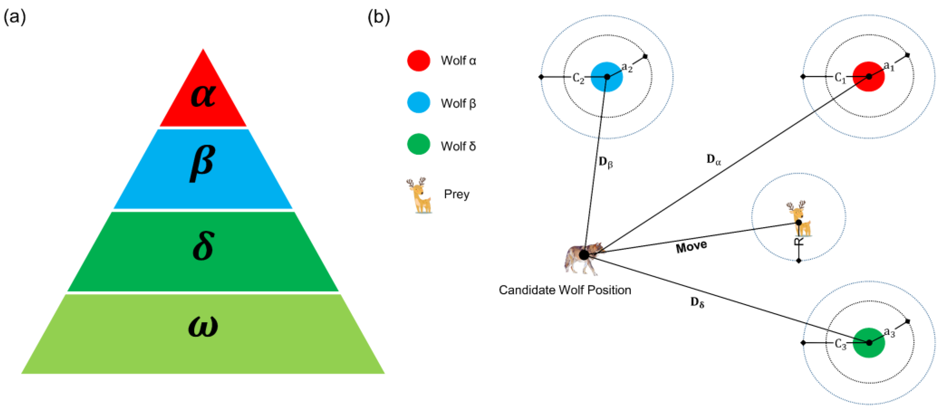
2.2. Grey Wolf Optimization

Grey Wolf Optimization (GWO) [25] was proposed by Mirjalili et al. in 2014, which mainly mimics the social leadership hierarchy and hunting mechanism of grey wolves in nature. Mirjalili et al. demonstrated that the optimization performance of standard GWO outperformed PSO, CS, and ABC algorithms, etc. Since GWO has the advantages of simple principle, fast seeking speed, fast convergence, few adaptive parameters, high search precision and easy implementation, it is easier to combine with practical engineering problems. Now it is widely used in feature selection [26], unmanned combat vehicle path planning [27], economic scheduling assignment [28], and multi-objective scheduling problems [29], etc.
The application where we use GWO for hyperparameter tuning is inspired by GWO combined with neural network [30]. This is because the main idea behind hyperparameter tuning is to find an optimum set of values for parameters in order to maximize the performance of a given neural network model or algorithm. Correspondingly, in this study the given model is LSTM. The inspiration for GWO is the behavior of the grey wolf, which is led by a small number of grey wolves (general three wolves) who move toward the prey, and the given model explores the search space in the hope of finding an optimal solution. There are two pivotal aspects of this behavior: social hierarchy and hunting mechanism, which are shown in Figure 2.
Naturally, a grey wolf pack is divided into four ranks because of its population hierarchy, which is shown in Figure 2a below. We consider the fittest solution as the wolf α , the second and third best solutions are named wolf β and wolf δ respectively. The rest of the candidate solutions are assumed to be wolves ω . The wolf α has absolute dominance over wolf β , wolf δ , and wolves ω , while wolf β has absolute dominance over wolf δ and wolves ω , and so on. In order to mathematically model the social hierarchy, we generally regard α , β , and δ as the best three fitness performance(optimal solutions) after each round of iteration; they guide the candidate wolves ( ω ) to update their positions to move toward the prey, as Figure 2b shows. Note that fitness refers to the mapping value obtained by substituting the value of the hyperparameters corresponding to the position of the grey wolf into the customized objective function (cost function, which is described in Section 2.4, Paragraph 1 and 2. Simply speaking, the process of grey wolves α , β , and δ leading the grey wolf pack moving toward the prey is the process of searching for the optimal hyperparameters.
Mentioned above, the hunting mechanism, i.e., the principle of the position updating rules is shown in Figure 2b. Where D α , D β , and D δ denote the distances between wolves α , β , and δ and the candidate wolf individual respectively; C 1 , C 2 , and C 3 are the random weights of the grey wolf position; a 1 , a 2 , and a 3 represent the convergence factors, which have the same values and can be denoted uniformly by a , decreasing linearly from 2 to 0 as the number of iteration increases.
To mathematically model Figure 2b, we need to suppose the position vectors of wolves α, β, and δ in the d -dimensional space are shown in Formula (1), where 1 ≤ k d , indicating the k th dimensional component in the d -dimensional space. d also denotes the number of hyperparameters to be optimized, e.g., in this study, we need to realize the automatic search of the number of hidden units (hu) and learning rate (lr) for optimization by GWO, so d is 2. Note that the following formulas or equations in this section that we proposed are based on code, so from that viewpoint, these formulas are not the same as those in other papers.
{ X α : ( X α , 1 , X α , 2 , , X α , d ) X β : ( X β , 1 , X β , 2 , , X β , d ) X δ : ( X δ , 1 , X δ , 2 , , X δ , d )
Meanwhile, suppose the current position vector of a candidate wolf i is X i ( X i , 1 , X i , 2 , , X i , d ) , and its next position vector under the joint leadership of wolves α , β, and δ is X i ( X i , 1 , X i , 2 , , X i , d ) . The calculation procedures of each dimensional component X i , k of X i are presented in Formulas (2)–(5):
{ X α i , k = X α , k A 1 · D α , k D α , k = | C 1 · X α , k X i , k | C 1 = 2 r 2 A 1 = 2 a · r 1 a
{ X β i , k = X β , k A 2 D β , k D β , k = | C 2 X β , k X i , k | C 2 = 2 r 2 A 2 = 2 a r 1 a  
{ X δ i , k = X δ , k A 3 D δ , k D δ , k = | C 3 X δ , k X i , k | C 3 = 2 r 2 A 3 = 2 a r 1 a
X i , k = X α i , k + X β i , k + X δ i , k 3  
First, D α , 1 and X α i , 1 were calculated as shown in Formula (2), the former denotes the distance between the corresponding dimensional value of grey wolf α:   X α , 1 multiplied by the influence weight C 1 . and the corresponding dimensional value of candidate wolf i :   X i , 1 at the 1st dimensional component and takes its absolute value as D α , 1 ; The latter likewise represents the next position of candidate wolf i under the guidance of grey wolf α at the 1st dimensional component, which is X α i , 1 . By analogy, the next positions of candidate wolf i under the guidance of grey wolf β and δ at the 1st dimensional component, X β i , 1 and X δ i , 1 , respectively, are calculated as shown in Formulas (3) and (4). Then X α i , 1 , X β i , 1 , and X δ i , 1 were averaged to obtain X i , 1 , as shown in Formula (5), that is, the next position (new position) of candidate wolf i at the 1st dimensional component under the joint leadership of grey wolf α, β, and δ is obtained. By analogy, a total of d new positions, namely X i , 1 , X i , 2 , and X i , d are obtained, they form the latest position vector of candidate wolf i during that round of iteration.
In Formulas (2)–(5), A 1 ,   A 2 ,   A 3 ,   C 1 ,   C 2 ,   C 3 ,   r 1 ,   r 2 and a all represent one value, where C 1 ,   C 2 ,   C 3 are calculated from different r 2 values, and the same for A 1 ,   A 2 ,   A 3 . Both r 1 and r 2 are random numbers between 0 and 1. During each iteration of the algorithm, the position space dimension of each grey wolf is traversed, and different r 1 and r 2 are randomly generated for the computation of X α i , k ,   X β i , k and X δ i , k , while a decreases from 2 to 0 with the increasement of iterations. ‘|’ stands for taking absolute values and ‘ , ’ stands for multiplication.
However, the shortcomings of GWO cannot be ignored. For example, Niu et al. found that the farther the function’s optimal solution is from 0, the worse its performance [31]; Zhang et al. summarized that GWO has poor population initialization, unavoidable falling into the local optimum, etc. [32]. Consequently, a lot of works have been conducted to improve GWO, e.g., Yang et al. proposed Group GWO to realize a better global convergence [33]; Gao et al. proposed VW-GWO to reduce the probability of being trapped in local optima [34]; Mehrotra et al. put forward Chaos GWO to improve the ability to escape local optima by replacing the key parameters by chaotic variables [35]; Malik et al. [36] proposes the Weighted Distance GWO to modify the grey wolf position updating strategy and the weighted sum of best positions is used instead of just a simple average, turning out to have a superior performance compared to standard GWO, etc.

2.3. LSTM

Long short term memory (LSTM) [37] network is a special kind of recurrent neural network (RNN) capable of learning order dependencies in sequence prediction problems. This is the pattern mechanism needed for complex problem areas such as machine translation and speech recognition, etc. LSTM can efficiently deliver and express information in long time sequences, and it may keep information for a long time by default. In short, LSTM addresses the issue of RNN long-term dependency. At the same time, it overcomes the two technical problems of vanishing gradients and exploding gradients when training [38,39]. This is why LSTM is used for time-series data processing, prediction, and classification [40]. So back to the present experiment, in Section 2.1, we briefly describe the processing of the raw data to obtain a standard time-series type data format that can be fed into the LSTM neural network model for training, i.e., each audio is processed as a matrix of frames × number. We got the idea that now that LSTM might be able to connect previous information to the present task, the same as using previous audio frames might inform the understanding of the present frame, we thought it would be reasonable to apply LSTM in this study. Thus, we chose to use LSTM for modeling.
The key to the LSTM solution to the problems mentioned above is the specific internal structure of the cells used in the network. Its architecture is shown in Figure 3 below. The key to the LSTM is the cell state, the horizontal line that runs across the top of the chart, from C t 1 to C t . For all LSTM cells (LSTM cell chain), the cell state is like a conveyor belt, which travels straight along the entire LSTM cell chain, and information can easily flow along it unchanged. We can see that each LSTM cell has three gates: the forget gate, the input gate, and the output gate. Gates are a way to optionally allow information to pass through, and they are composed of a sigmoid neural net layer (i.e., logistic activation function) and a pointwise (i.e., element-wise) multiplication operation (i.e., Hadamard Product). The sigmoid layer outputs numbers between 0 and 1 that describe the degree to which each component should be allowed to be let through. A value of 0 means letting nothing through, while a value of 1 means letting everything through. They are designed to protect and control the cell state.
For other Identifier characters in the figure, the X t and h t 1 are the input vectors, where the variable t is the timestamp (time step). We can think of h t as the short-term state and c(t) as the long-term state, y t likewise represents the short-term state, which is equal to the cell’s output for this time step, while h t serves as the input for the next timestamp, which means current h t is the next cell’s h t 1 . The computation of each cell can be defined by the following Equations (6)–(11):
f t & = σ ( W f [ h t 1 , x t ] + b f )
g t & = tan h ( W g [ h t 1 , x t ] + b g )  
i t & = σ ( W i [ h t 1 , x t ] + b i )  
o t & = σ ( W o [ h t 1 , x t ] + b o )  
c t & = f t     C t 1 + g t     i t
y t & = tan h ( c t )     o t
where ‘ ’ denotes the multiplication of matrix, please note the distinction between the symbol ‘ ’; f t , g t , i t , o t are obtained by feeding the current input vector x t and the previous short-term state h t 1 into four different fully connected layers (i.e., FC in the figure); W f , W g , W i , and W o are the weight matrices; b f , b g , b i , and b o are the bias terms for each of the four layers. In short, with the function of these three gates, the LSTM cells can capture and learn the complex correlation features in the short or long term time series, audio recordings, and more [42].

2.4. GWO + LSTM Algorithm

In this study, we simulate the LSTM 2 hyperparameter hidden units (hu) and learning rate (lr) as the prey of the grey wolf pack. The algorithm flowchart of GWO combined with the LSTM neural network is shown in Figure 4. It shows that before the condition of iterations is satisfied, i.e., in the iterative searching process, GWO will keep delivering hyperparameters to LSTM model for training, and the trained model will keep returning the fitness value which is obtained by evaluation on the val set through a cost function as follows:
fitness   = 1 accuracy
More specifically, accuracy is the ratio of the number of correct model predictions to the number of samples in the validation set compared to the true labels in the validation set, refer to the confusion matrix [43] for a comprehensive explanation. So, for the model, the larger the accuracy is, the better. Correspondingly, the smaller the fitness is, the better. The cost function is customized by users as long as the design of it is reasonable. It is the criteria of the GWO + LSTM process.
In each iteration, GWO will traverse every wolf of the pack and obtain the wolf’s fitness, then we determine the top three wolves according to the best three fitness values as α , β , and δ . The specific process is divided into the following steps.
  • Initialize the GWO parameters (e.g., a ,   A , C ) and configure some parameters of the LSTM. For GWO, we set the grey wolf pack size to 5, the number of LSTM hyperparameters (hu and lr) to be optimized to 2, the upper and lower search (i.e., optimization) spaces to hu and lr, which are self-defined in Table 1 below. Initialize the spatial position of the wolf population, in this study this is a (5, 2) matrix, noting that the dimension of the spatial location is the number of hyperparameters to be optimized. Set the max iterations to 5, which is the termination condition of the algorithm. For the LSTM neural network, set the epoch to 5 and batch size to 16
  • In each iteration, hyperparameters represented by every grey wolf position are substituted into the LSTM model for training and evaluation. In this step the train set is input into the LSTM model for training. Further, the trained model is utilized to evaluate the val data to obtain the accuracy metric. Next, according to Equation (6), we get the fitness of every wolf in this iteration. The smaller the fitness we get, the better the performance of the trained model we have. Finally, the three wolves with the smallest fitness in this iteration are selected or regarded as wolves α , β , and δ
  • The top three wolves α , β , δ selected from step 2 lead the grey wolf pack to search for prey, and the position of each grey wolf is updated and changed according to Formulas (2)–(5)
  • Repeat the above steps 2–3 until the termination condition (i.e., the max iterations) is met. The hyperparameter corresponding to the position of the final output wolf α is the optimal hyperparameter of the LSTM model obtained by GWO searching. It is worth noting that for the process of GWO, it can be considered that the grey wolf position denotes the hyperparameter vector; after GWO completes all the iterations, wolf α ’s position denotes both the prey position and the optimal hyperparameter vector.

3. Results

3.1. Comparison of Quantitative Results of Model Performance

In this experiment, the default setting of the grey wolf pack size is 5, i.e., there are 5 wolves in the pack, and the max iterations of GWO is 5. With the increment of iteration, the model’s fitness variation is illustrated as in Figure 5 below. It shows the change in the best fitness value of the model with increasing number of iterations during each iteration. We can see that fitness becomes smaller and smaller from the first iteration to the second, and finally smooths out. Out of the randomness of GWO mechanics, the final optimal solution found by the GWO algorithm will be different because of setting different grey wolf pack sizes and iterations, which will be discussed centrally in Section 4. The curve in Figure 5 will expectedly continue to decrease and level off as the iteration increases, but relatively, more time and computational resource will be consumed.
Finally, the best combination of hyperparameters (i.e., optimal solution or position vector or hyperparameter vector) found by GWO + LSTM is shown in Table 2, hu is 185, lr is 0.1. Apart from hu and lr, any other parameters remain unchanged compared to the baseline LSTM model. In addition, we compiled the statistics of hyperparameter searching time by GWO in the Tables of Section 4.
According to Table 2, we use the best hyperparameter combination (185, 0.1) to configure LSTM neural network as “GWO + LSTM model”, and carry out 100 times 10-fold cross-validation on the train set base on the GWO + LSTM model and baseline LSTM model, respectively. Next, all evaluation metrics of both models on the train set and test set are statistical averaged and then summarized as Table 3. We can see that GWO + LSTM metric results are 2% higher than those of the baseline (benchmark) LSTM model, which is a very good improvement. Note that the metric of training time does not make any sense, we believe this is due to the small amount of data, the epoch of 10 (relatively small), and the GPU computing power, so that we cannot see a significant difference in training time.

3.2. Comparison of Visualization Results

The implicit state information output by the hidden layer of the LSTM model at the last moment (in this study, i.e., the frame) is indicated by h t , which represents the abstract features of the time series. h t contains key information such as the trend and history of the time series, which have an important impact on the final classification results of the model. In order to observe whether the abstract features output by baseline LSTM and GWO + LSTM models are distinguishable, in this subsection, we randomly select 200 samples from the test set, including 100 lightning whistler wave samples and 100 non-lightning whistler wave samples, and input these samples into the baseline LSTM model and GWO + LSTM model to extract hidden layer information features h t , and visualize them for comparison, as shown in Figure 6. Where the horizontal axis represents the number of hidden units and the sequence length of h t as well, the vertical axis represents the abstract feature values. It can be seen that the density of abstract feature sequences of the lightning whistler wave and non-lightning whistler wave are different between the baseline LSTM model and the GWO + LSTM model: The former model has a smaller inter-class variance along with a larger intra-class variance, while the latter has a larger inter-class variance and a smaller intra-class variance, indicating that the features learned by the GWO + LSTM model find it easier to achieve the classification of lightning whistler wave.
Next, the hidden layer feature information h t is input to the final fully connected layer to obtain the prediction scores between 0 and 1, as shown in Figure 7. Where the horizontal axis represents the sample serial number, and the vertical axis represents the probability value obtained from the h t hidden layer state information calculated by the sigmoid function of the fully connected layer. It can be seen that the classification effect of GWO + LSTM is significantly better than baseline LSTM, and the distribution points of lightning and non-lightning whistler waves are more distinct. This verifies the fact we elaborated on in Figure 6, which is powerful evidence for the model recognition results.

4. Discussion

For the GWO algorithm itself, its automatic searching results, i.e., the optimized(optimal) hyperparameters (hu and lr), their quality is affected by the size of the grey wolf pack (number of grey wolves) and iterations of the algorithm. In this experiment, in order to observe the model effect (fitness) by setting different pack size and iterations, on the basis of the above experiment that sets the grey wolf pack size and iterations each to 5, we use the control variate method to set pack size and the iterations increased from 5 to 12 respectively. The results are illustrated in Figure 8. This shows that the fitness curve only decreases and tends to be smooth as the pack size or iterations increase. It is worth noting that the initial position of the fitness is not immobile, which is caused by the random initialization of the parameters of the GWO algorithm itself. In addition, due to the searching mechanism of GWO, a locally optimal solution might be generated, which leads to a special state where part of the curves in the figure is a straight line from the beginning to the end of the max iterations only.
Then, the models are trained with the hyperparameter combinations optimized by GWO under the circumstance of setting different parameters (pack size and iterations). After performing 100 times of 10-fold cross-validation, the recognition effects (evaluation metrics) on the test set were averaged and are summarized in Table 4 and Table 5. By observing Table 4, as the pack size increases, AUC (area under curve), accuracy and F1score are all stable above 0.95, precision is above 0.93 and recall is above 0.97 compared with the metrics corresponding to (pack size, iterations) of (5, 5). Among them, note that the hyperparameter combinations with (hu, lr) of (182, 0.1), (177, 0.1), and (181, 0.1) were obtained under the parameter configurations of (7, 5), (8, 5), and (9, 5) respectively, especially, their lr value is the upper limit of the learning rate range that we customed in Table 1. So, we can see that the algorithm still has room for improvement, which can be achieved by continuing to expand the upper and lower searching space limits of the hyperparameters. Similarly, by observing Table 5, it is found that the experimental results of all combinations of GWO parameters (pack size, iterations) on the test set are 2% higher than those of the baseline LSTM model for each metric. As iterations increase, the improvement effect is basically no different from that in Table 4 compared with the original (pack size, iterations) of (5, 5). Analyzed from time perspective, for one aspect, the difference in hyperparameter searching time between Table 4 and Table 5 is not significant, but we can see that as the pack size or iterations increase, the searching time for hu and lr also increases, which occurs as expected. For another aspect, the training time in the two tables almost makes no difference under the condition of same batch size, epoch, etc., and the corresponding (hu, lr).
Therefore, it can be inferred that the model effect can be further improved by increasing the number of pack size and iterations, which indicates that the GWO + LSTM model can more reliably solve the problem in that the neural network model relies on manual tuning hyperparameters and realizes the function of automatic tuning and then optimizes the model. However, limitations exist. First, we have only reproduced the standard GWO algorithm, and then used it for the hyperparametric optimization aspect of this experiment. Although we have achieved the desired experimental results, we have not made improvements to the algorithm itself. For example, one of the shortcomings of GWO is the randomness problem at initialization, which can lead to the search results falling into local optima, etc. Second, since this experiment is based on the baseline model proposed by Yuan et al., the neural network architecture used is not complex, consisting of only one LSTM hidden layer and one dense layer. If the model structure is more complex that is with multiple layers, it will bring more complexity, including the choice of hyperparameters, the need to optimize, and time complexity. Third, the comparisons in Section 3 could be made with more candidate algorithms and not just limited to LSTM and GWO + LSTM. We can add such as PSO + LSTM, (Cuckoo Algorithm) CA + LSTM, etc., to this experiment. Although our main goal in this study is to highlight the superiority of GWO + LSTM over LSTM, adding other algorithms appropriately would enrich the completeness of the experiment and strengthen this paper. To improve and address these three points, we need to take them into consideration in future studies.

5. Conclusions

This paper addresses the problem that hyperparameters need to rely on manual repetition of multiple experiments to determine them, and proposes the lightning whistler wave recognition model based on GWO. The method simulates the process of searching for the optimal hyperparameters as in the process of the grey wolves with absolute dominance leading the wolf pack to move towards the prey and achieves the purpose of automatically finding the optimal hyperparameters of the lightning whistler wave recognition model. The experimental results prove that the recognition effect is better than that of manually setting hyperparameters: Compared with the lightning whistler wave recognition model with hyperparameters based on manual settings, the model with hyperparameters optimized by GWO proposed in this study has a 2% improvement in AUC, accuracy, F1 score, precision, and recall metrics.
Applying the algorithm scheme proposed in this study, deploying, and piggybacking it in a satellite-based system will further improve the accuracy of the lightning whistler wave recognition model for satellite-based applications, which will promote the subsequent development of related research. Thus, we can collect more pure lightning whistler wave data, which will provide crucial data support to research the relations between the spatial and temporal patterns of the lightning whistler wave and atmospheric particles, climate change, and earthquake occurrence. In addition, the core part of this study—automatic hyperparameter searching based on the GWO algorithm, in addition to the optimization of the number of hidden units and learning rate of the LSTM neural network that we selected in this study—can also be used to search for the LSTM dropout for optimization. According to different application requirements, it can also be applied to hyperparameter optimization of neural networks such as CNN (convolutional neural networks) and GRU (gate recurrent unit) to improve model performances
In the future, the algorithm can be optimized in the following two aspects. One is the optimization based on the GWO algorithm itself, including the improvement of the space position’s initialization of the grey wolf pack, the wolves’ hunting mechanism, etc. In this study, we set the same number of lightning whistler waves and non-lightning whistler waves in the validation set, train set, and test set. However, in the actual spatial magnetic field environment, the collected audio samples are completely unbalanced, and the non-lightning whistler wave data occupy most of them. Thus, the class weights can be adjusted by modifying the cross-entropy loss function to solve the problem of unbalanced samples in real scenarios.

Author Contributions

Conceptualization, J.Y.; methodology, J.Y. and C.L.; validation, J.W.; formal analysis, J.Y.; investigation, C.L. and J.W.; resources, Q.W., Z.Z., J.H. and X.S.; data curation, J.Y. and C.L.; writing—original draft preparation, C.L. and J.W; writing—review and editing, J.Y., Y.H. and Q.W.; visualization, C.L.; supervision, J.F. and Y.W.; project administration, J.Y. and Q.W.; funding acquisition, Q.W. All authors have read and agreed to the published version of the manuscript.

Funding

This research was supported by grants from the National Natural Science Foundation of China (42104159), the Hebei Higher Education Teaching Reform Research and Practice Project (2021GJJG486).

Institutional Review Board Statement

Not applicable.

Informed Consent Statement

Not applicable.

Data Availability Statement

The data reported in this study are available on request from the corresponding author.

Acknowledgments

Special thanks to all members of the ZH-1 team from the National Institute of Natural Hazards, Ministry of Emergency Management of China, for their technical service support of the research data in this paper. We also thank the reviewers for their constructive comments and suggestions, which resulted in a significant improvement in the quality of the paper. It is beyond words in thanking the assigned editor and other editors for their kind reminders and sense of responsibility.

Conflicts of Interest

The authors declare no conflict of interest.

References

  1. Helliwell, R. Whistlers and Related Ionospheric Phenomena; Courier Corporation: Chelmsford, MA, USA, 1965. [Google Scholar]
  2. Rycroft, M.J. Some Effects in the Middle Atmosphere Due to Lightning. J. Atmos. Terr. Phys. 1994, 56, 343–348. [Google Scholar] [CrossRef]
  3. Bayupati, I.P.A.; Kasahara, Y.; Goto, Y. Study of Dispersion of Lightning Whistlers Observed by Akebono Satellite in the Earth’s Plasmasphere. IEICE Trans. Commun. 2012, E95.B, 3472–3479. [Google Scholar] [CrossRef] [Green Version]
  4. Oike, Y.; Kasahara, Y.; Goto, Y. Spatial Distribution and Temporal Variations of Occurrence Frequency of Lightning Whistlers Observed by VLF/WBA Onboard Akebono. Radio Sci. 2014, 49, 753–764. [Google Scholar] [CrossRef]
  5. Yuan, J.; Wang, Q.; Yang, D.; Liu, Q.; Zhima, Z.; Shen, X. Automatic recognition algorithm of lightning whistlers observed by the Search Coil Magnetometer onboard the Zhangheng-1 Satellite. Chin. J. Geophys. 2021, 64, 3905–3924. [Google Scholar]
  6. Shen, X.H.; Zhang, X.M.; Cui, J.; Zhou, X.; Jiang, W.L.; Gong, L.X.; Liu, Q.Q. Remote sensing application in earthquake science research and geophysical fields exploration satellite mission in China. J. Remote Sens. 2018, 22, 1–16. [Google Scholar]
  7. Zhang, X.M.; Qian, J.D.; Shen, X.H.; Liu, J.; Wang, Y.L.; Huang, J.P.; Zhao, S.F.; Ouyang, X.Y. The Seismic Application Progress in Electromagnetic Satellite and Future Devel-opment. Earthquake 2020, 40, 18–37. [Google Scholar]
  8. Luo, X.; Niu, S.; Zuo, Y.; Tao, Y. Simulation of high-energy electron diffusion in the inner radiation belt based on AKEBONO whistler wave parameters. Comput. Phys. 2017, 34, 335–343. [Google Scholar] [CrossRef]
  9. Horne, R.B.; Glauert, S.A.; Meredith, N.; Boscher, D.; Maget, V.; Heynderickx, D.; Pitchford, D. Space Weather Effects on Satellites and Forecasting the Earth’s Electron Radiation Belts with SPACECAST. Space Weather 2013, 11, 169–186. [Google Scholar] [CrossRef] [Green Version]
  10. Yuan, J.; Wang, Q.; Zhang, X.; Yang, D.; Wang, Z.; Zhang, L.; Shen, X.; Zeren, Z. Advances in the automatic detection algorithms for lightning whistlers recorded by electromagnetic satellite data. Chin. J. Geophys. 2021, 64, 1471–1495. [Google Scholar]
  11. Wang, Q.; Huang, J.; Zhang, X.; Shen, X.; Yuan, S.; Zeng, L.; Cao, J. China Seismo-Electromagnetic Satellite search coil magnetometer data and initial results. Earth Planet. Phys. 2018, 2, 462–468. [Google Scholar] [CrossRef]
  12. Yuan, J.; Wang, Z.; Zeren, Z.; Wang, Z.; Feng, J.; Shen, X.; Wu, P.; Wang, Q.; Yang, D.; Wang, T.; et al. Automatic recognition algorithm of the lightning whistler waves by using speech processing technology. Chin. J. Geophys. 2022, 65, 882–897. [Google Scholar] [CrossRef]
  13. Begam, M. Voice Recognition Algorithms Using Mel Frequency Cepstral Coefficient (MFCC) and Dynamic Time Warping (DTW) Techniques. Comput. Res. Repos. 2010, 2, 138–143. [Google Scholar]
  14. Yang, F.; Wang, P.; Zhang, Y.; Zheng, L.; Lu, J. Survey of Swarm Intelligence Optimization Algorithms. In Proceedings of the 2017 IEEE International Conference on Unmanned Systems (ICUS), Beijing, China, 27–29 October 2017; pp. 544–549. [Google Scholar]
  15. Kandasamy, P. Literature Review on Grey Wolf Optimization Techniques. Int. J. Sci. Res. (IJSR) 2020, 9, 1765–1769. [Google Scholar]
  16. Kennedy, J.; Eberhart, R. Particle Swarm Optimization. In Proceedings of the ICNN’95—International Conference on Neural Networks, Perth, Australia, 27 November–1 December 1995; Volume 4, pp. 1942–1948. [Google Scholar]
  17. Karaboga, D.; Basturk, B. Artificial Bee Colony (ABC) Optimization Algorithm for Solving Constrained Optimization Problems. In Foundations of Fuzzy Logic and Soft Computing; Springer: Berlin/Heidelberg, Germany, 2007; pp. 789–798. [Google Scholar]
  18. Dorigo, M.; Birattari, M.; Stutzle, T. Ant Colony Optimization. IEEE Comput. Intell. Mag. 2006, 1, 28–39. [Google Scholar] [CrossRef]
  19. Eusuff, M.; Lansey, K.; Pasha, F. Shuffled Frog-Leaping Algorithm: A Memetic Meta-Heuristic for Discrete Optimization. Eng. Optim. 2006, 38, 129–154. [Google Scholar] [CrossRef]
  20. Yang, X.-S.; Deb, S. Cuckoo Search via Lévy Flights. In Proceedings of the 2009 World Congress on Nature & Biologically Inspired Computing (NaBIC), Coimbatore, India, 9–11 December 2009; pp. 210–214. [Google Scholar]
  21. Wang, J.-S.; Li, S.-X. An Improved Grey Wolf Optimizer Based on Differential Evolution and Elimination Mechanism. Sci. Rep. 2019, 9, 7181. [Google Scholar] [CrossRef]
  22. Zhou, B.; Yang, Y.; Zhang, Y.; Gou, X.; Cheng, B.; Wang, J.; Li, L. Magnetic Field Data Processing Methods of the China Seismo-Electromagnetic Satellite. Earth Planet. Phys. 2018, 2, 455–461. [Google Scholar] [CrossRef]
  23. Molau, S.; Pitz, M.; Schluter, R.; Ney, H. Computing Mel-Frequency Cepstral Coefficients on the Power Spectrum. In Proceedings of the 2001 IEEE International Conference on Acoustics, Speech, and Signal Processing, Proceedings (Cat. No. 01CH37221), Salt Lake City, UT, USA, 7–11 May 2001; Volume 1, pp. 73–76. [Google Scholar]
  24. Browne, M.W. Cross-Validation Methods. J. Math. Psychol. 2000, 44, 108–132. [Google Scholar] [CrossRef] [Green Version]
  25. Mirjalili, S.; Mirjalili, S.M.; Lewis, A. Grey Wolf Optimizer. Adv. Eng. Softw. 2014, 69, 46–61. [Google Scholar] [CrossRef] [Green Version]
  26. Emary, E.; Zawbaa, H.M.; Grosan, C.; Hassenian, A.E. Feature Subset Selection Approach by Gray-Wolf Optimization. In Afro-European Conference for Industrial Advancement; Springer: Cham, Switzerland, 2015; pp. 1–13. [Google Scholar] [CrossRef]
  27. Zhang, S.; Zhou, Y.; Li, Z.; Pan, W. Grey Wolf Optimizer for Unmanned Combat Aerial Vehicle Path Planning. Adv. Eng. Softw. 2016, 99, 121–136. [Google Scholar] [CrossRef] [Green Version]
  28. Song, H.; Sulaiman, M.; Mohamed, M.R. An Application of Grey Wolf Optimizer for Solving Combined Economic Emission Dispatch Problems. Int. Rev. Model. Simulations (IREMOS) 2014, 7, 838. [Google Scholar] [CrossRef]
  29. Lu, C. Research on Multi-Objective Shop Scheduling Problem with Controllable Processing Time. Ph.D. Thesis, Huazhong University of Science and Technology, Wuhan, China, 2017. [Google Scholar]
  30. Sánchez, D.; Melin, P.; Castillo, O. A Grey Wolf Optimizer for Modular Granular Neural Networks for Human Recognition. Comput. Intell. Neurosci. 2017, 2017, e4180510. [Google Scholar] [CrossRef] [PubMed] [Green Version]
  31. Niu, P.; Niu, S.; Liu, N.; Chang, L. The Defect of the Grey Wolf Optimization Algorithm and Its Verification Method. Knowl.-Based Syst. 2019, 171, 37–43. [Google Scholar] [CrossRef]
  32. Zhang, X.F.; Wang, X.Y. Review of Gray Wolf Optimization Algorithm Research. Comput. Sci. 2019, 46, 30–38. [Google Scholar]
  33. Yang, B.; Zhang, X.; Yu, T.; Shu, H.; Fang, Z. Grouped Grey Wolf Optimizer for Maximum Power Point Tracking of Doubly-Fed Induction Generator Based Wind Turbine. Energy Convers. Manag. 2017, 133, 427–443. [Google Scholar] [CrossRef]
  34. Gao, Z.-M.; Zhao, J. An Improved Grey Wolf Optimization Algorithm with Variable Weights. Comput. Intell. Neurosci. 2019, 2019, e2981282. [Google Scholar] [CrossRef]
  35. Mehrotra, H.; Pal, S.K. Using Chaos in Grey Wolf Optimizer and Application to Prime Factorization. In Soft Computing for Problem Solving; Springer: Singapore, 2019; pp. 25–43. [Google Scholar] [CrossRef] [Green Version]
  36. Malik, M.R.S.; Mohideen, E.R.; Ali, L. Weighted Distance Grey Wolf Optimizer for Global Optimization Problems. In Proceedings of the 2015 IEEE International Conference on Computational Intelligence and Computing Research (ICCIC), Madurai, India, 10–12 December 2015; pp. 1–6. [Google Scholar]
  37. Hochreiter, S.; Schmidhuber, J. Long Short-Term Memory. Neural Comput. 1997, 9, 1735–1780. [Google Scholar] [CrossRef]
  38. Graves, A.; Liwicki, M.; Fernández, S.; Bertolami, R.; Bunke, H.; Schmidhuber, J. A Novel Connectionist System for Unconstrained Handwriting Recognition. IEEE Trans. Pattern Anal. Mach. Intell. 2009, 31, 855–868. [Google Scholar] [CrossRef] [Green Version]
  39. Gers, F.A.; Schmidhuber, J.; Cummins, F. Learning to Forget: Continual Prediction with LSTM. Neural Comput. 2000, 12, 2451–2471. [Google Scholar] [CrossRef]
  40. Gers, F.A.; Eck, D.; Schmidhuber, J. Applying LSTM to Time Series Predictable Through Time-Window Approaches. In Neural Nets WIRN Vietri-01; Springer Science & Business Media: Berlin/Heidelberg, Germany, 2002; pp. 193–200. [Google Scholar] [CrossRef]
  41. Pan, J.; Jing, B.; Jiao, X.; Wang, S. Analysis and Application of Grey Wolf Optimizer-Long Short-Term Memory. IEEE Access 2020, 8, 121460–121468. [Google Scholar] [CrossRef]
  42. Yu, Y.; Si, X.; Hu, C.; Zhang, J. A Review of Recurrent Neural Networks: LSTM Cells and Network Architectures. Neural Comput. 2019, 31, 1235–1270. [Google Scholar] [CrossRef] [PubMed]
  43. Ruuska, S.; Hämäläinen, W.; Kajava, S.; Mughal, M.; Matilainen, P.; Mononen, J. Evaluation of the Confusion Matrix Method in the Validation of an Automated System for Measuring Feeding Behaviour of Cattle. Behav. Process. 2018, 148, 56–62. [Google Scholar] [CrossRef] [PubMed]
Figure 1. Architecture as well as the methodological steps of the lightning whistler wave recognition scheme. Overall, the flow chart comprises three procedures: model hyperparameter optimization flow, model training flow, and model application flow. The input of the model is the feature map matrix extracted from wave audio, and the output (i.e., likelihood value from 0 to 1) denotes whether the wave is lightning whistler wave or not.
Atmosphere 13 01828 g001
Figure 2. The intro-diagrams of GWO including (a) the social hierarchy of grey wolf pack (dominance decreases from top down) and (b) diagram of the hunting mechanism, as well as the grey wolf position updating process. “Readapted with permission from Ref. [25]. 2022, Elsevier”.
Atmosphere 13 01828 g002
Figure 3. The internal structure of the LSTM cell. “Readapted with permission from Ref. [41]. 2022, Pan et al.”.
Atmosphere 13 01828 g003
Figure 4. Hyperparameters optimization process by GWO with LSTM. “Readapted with permission from Ref. [41]. 2022, Pan et al.”
Atmosphere 13 01828 g004
Figure 5. Wolf α’s fitness performance variation along the process of GWO iterations.
Atmosphere 13 01828 g005
Figure 6. Hidden layer h t state information feature diagram.
Atmosphere 13 01828 g006
Figure 7. The output value of h t at the fully connected layer.
Atmosphere 13 01828 g007
Figure 8. The fitness variation of the model with the increment of iterations by setting different hyperparameters. The left one denotes controlling the grey wolf pack size to 5, the right one denotes controlling the iterations to 5.
Atmosphere 13 01828 g008
Table 1. The upper and lower search space corresponding to the hyperparameter to be optimized.
Hyperparameters to Be OptimizedSearching Space
The number of hidden units (hu)(64, 256)
learning rate (lr)(0.01, 0.1)
Table 2. Comparison of (hu, lr) before and after GWO optimized LSTM.
AlgorithmhulrBatchEpochOptimizerLoss Function
Parameters
LSTM1280.011610Adagradbinary_cross entropy
GWO + LSTM1850.11610Adagradbinary_cross entropy
Table 3. Comparison of the average metrics before and after GWO optimized LSTM.
DataAlgorithm(hu, lr)Training
Time (min) *
Evaluation Metrics
AUCAccuracyF1 ScorePrecisionRecall
Train setLSTM(128, 0.01)0.270.96270.96370.96210.94650.9787
GWO + LSTM(185, 0.1)0.220.97710.97750.97670.96350.9904
Test setLSTM--0.93340.93540.93160.90780.9577
GWO + LSTM--0.9540.95510.95290.93190.9752
* Single training time of model without cross-validation. Experimental GPU environment: NVIDIA GeForce RTX 2080 Ti.
Table 4. Hu and lr obtained under different pack size and the experimental results.
Pack
Size
Iterations(hu, lr)Searching
Time (min) 1
Training Time (min) 2Evaluation Metrics
AUCAccuracyF1 ScorePrecisionRecall
55(185, 0.1)2.880.220.9540.95510.95290.93190.9752
65(197, 0.048)3.560.20.95320.95440.95220.93380.9721
75(182, 0.1)4.20.20.95430.95530.95340.93530.9726
85(177, 0.1)4.730.180.95470.95560.95370.93470.9738
95(181, 0.1)5.440.180.95450.95570.95350.93340.9749
105(146, 0.08)5.960.180.95370.95470.95280.93460.972
115(201, 0.098)6.560.190.9540.95520.95310.93340.974
125(187, 0.098)7.150.190.95420.95540.95320.93340.9743
1 The searching time of optimal solution (hu, lr). 2 Single training time of model without cross-validation.
Table 5. Hu and lr obtained under different iterations and the experimental results.
Pack SizeIterations(hu, lr)Searching
Time (min)
Training Time (min)Evaluation Metrics
AUCAccuracyF1 ScorePrecisionRecall
55(185, 0.1)2.880.220.9540.95510.95290.93190.9752
56(191, 0.095)3.490.190.9550.9560.9540.9350.9741
57(87, 0.059)3.940.180.95270.95390.95170.93210.9725
58(131, 0.049)4.730.180.95040.95190.94930.92880.9714
59(167, 0.096)4.80.180.95420.95530.95320.93390.9738
510(117, 0.0725.570.190.95350.95440.95270.93640.9699
511(146, 0.064)6.100.190.95250.95380.95140.92950.9747
512(145, 0.080)6.850.190.9550.9560.9540.93480.9743
Publisher’s Note: MDPI stays neutral with regard to jurisdictional claims in published maps and institutional affiliations.

