Article

A Numerically Sensitive Study of Two Continuous Heavy-Pollution Episodes in the Southern Sichuan Basin of China

1
Yuhuan Meteorological Bureau, Taizhou 317600, China
2
State Key Laboratory of Severe Weather & Key Laboratory of Atmospheric Chemistry of CMA, Chinese Academy of Meteorological Sciences, Beijing 100081, China
3
Sichuan Key Laboratory of Plateau Atmosphere and Environment, Chengdu University of Information Technology, Chengdu 610225, China
*
Authors to whom correspondence should be addressed.
Atmosphere 2022, 13(11), 1771; https://doi.org/10.3390/atmos13111771
Submission received: 30 August 2022 / Revised: 23 October 2022 / Accepted: 24 October 2022 / Published: 27 October 2022
(This article belongs to the Special Issue Frontiers in Atmospheric Remote Sensing and Modelling)

Abstract

:
To explore the causes of pollution formation and changes in the complex topography of the Sichuan Basin, China, and improve the comprehensive simulation capability of pollution models, we use two online coupling models, WRF/Chem and WRF/CUACE, to simulate two heavy pollution episode that successively occurred in the southern part of Sichuan Province from 15 December 2016 to 11 January 2017 in this paper. Additionally, two sets of meteorological physics parameterization schemes MET1 and MET2 are designed, and four groups of experiments are carried out. The results suggest that the two models are good at simulating the static weather parameters such as temperature, low speed of winds and boundary layer height. The four groups of tests can accurately simulate the beginning, maintenance and turning point of the two pollution episodes’ life cycles. CUACE shows better performance in terms of higher correlation coefficients and lower errors in most of the particles and particulate components evaluations. It also performs better in the competitive mechanism of sulfate and nitrate against ammonium in the thermodynamic equilibrium mechanism. In addition, the evaluation of PM2.5 and the component simulation show that CUACE is more capable of simulating the mechanisms of heavy pollutions in southern Sichuan. Meanwhile, MET2 scheme is more appropriate for the simulation than MET1 dose. Based on the simulated concentrations of components and their precursors, the models overestimate the conversion of NO2 to nitrate but underestimate the conversion of SO2 to sulfate, which is the essential cause of the general overestimation of nitrate. Therefore, reducing the overestimation of nitrate is one major target for future model improvement.

1. Introduction

The Sichuan Basin, surrounded by high mountains, lies at the east edge of the Tibetan Plateau. With complex terrain, the thermodynamic and dynamic condition of atmosphere in the basin is very special and easy for static weather conditions characterized by weak wind speed and high relative humidity, to form. Such weather conditions are not conducive to the diffusion of pollutants [1], often causing serious pollution problems [2,3]. Affected by terrain factors, the vertical distribution and diffusion mechanisms of pollutants are more complex, and the observation is more difficult [4,5]. Thus, the Sichuan Basin has become one of the four major polluted regions in China [6]. Serious pollution problems, especially PM2.5 and O3, have an impact on people’s health [7]. The area is close to Tibet. The nature of the air pollution and how it is happened are very important for air pollution control and also for the interactions between the air pollution and the weather/climate in the region. The city cluster of southern Sichuan is located in the southern part of the Sichuan Basin, consisting of five prefecture-level cities, i.e., Zigong, Neijiang, Luzhou, Leshan, and Yibin. The visibility in this region has become very poor, close to or below 10 km all year round. Statistical analysis showed that the pollution in this area is mainly caused by high concentrations of PM2.5 or ozone [8,9,10]. The airflow enters the basin from the north and the east, and the pollutants spread to the southwest and then to the south along with the airflow, which tends to cause heavy pollution [11,12,13]. However, all the above findings were mainly based on statistical studies, and there are few in-depth studies on the interaction mechanism between heavy pollution and weather in southern Sichuan.
Numerical simulations can show good temporal and spatial continuity and pin down mechanizes behind them with variable physical and chemical schemes selected and evaluations [14]. The contributions of varying emission sources to PM2.5 in Dalian, Liaoning Province, in 2016 and the Beijing–Tianjin–Hebei region in 2018 were studied [15,16]. In terms of aerosol composition, simulation results revealed that nitrate is the main component of aerosols in the winter air pollution in Dalian [17]. In the Yangtze River Delta, several studies have used WRF-Chem to analyze the changes in ozone during the pollution process [18,19]. Fan et al. perform a numerical simulation analysis for three air pollution episodes in the Pearl River Delta (PRD) region during March 2012 using the third-generation air quality modeling system Models-3/CMAQ [20]. Chen et al. focused on the simulation of organic nitrates through a box model coupled with RACM2 (Regional Atmospheric Chemistry Mechanism, version 2) [21]. Wang et al. used WRF-Chem to investigate the sulfate formation mechanism [22]. The chemical schemes used in these studies were different [23], and few studies have been conducted on the changes of pollution and the effect of pollution on weather and climate in the heavily polluted Sichuan Basin, especially in southern Sichuan.
In this paper, we will use the WRF/Chem&CUACE to study two long-lasting pollution episodes in the southern Sichuan Basin from 15 December 2016 to 11 January 2017. Additionally, to pin down the mechanics of the heavy pollution in southern Sichuan Basin, the simulation capacity of the new comprehensive WRF/Chem&CUACE will be also investigated for its further improvement.

2. Experiments

2.1. Model Description

CMA Unified Atmospheric Chemistry Environment (CUACE) is an online chemical weather numerical prediction system developed by China Meteorological Administration (CMA) [24,25,26]. CUACE has been online coupled into version 3 of the Weather Research and Forecasting (WRF) community model that simulates trace gases and particulates simultaneously with meteorological fields [27], to build WRF/CUACE [28]. CUACE can simulate seven components of dust, black carbon (BC), organic carbon (OC), sulfate, nitrate, ammonium and sea salt. The aerosol microphysical processes include nucleation, hygroscopic growth, coagulation, condensation, and dry/wet deposition. The equilibrium scheme ISORROPIA (a new thermodynamic equilibrium model for multiphase multicomponent inorganic aerosols) [29,30] is applied to calculate nitrate and ammonium. The particle dry-deposition scheme developed by Petroff et al. [31] was introduced in the coupling model WRF-CUACE, and the distribution of the vegetation leaf area index (LAI) was improved by using MODIS data [32]. In CUACE, the heterogeneous chemical processes of SO2, NO2 and O3 on the surfaces of aerosols are taken into account, and the simulation effect of gases and secondary aerosols such as sulfate and nitrate is improved [33]. The aerosol mass spectrum is divided into 12 bins: 0.01–0.02, 0.02–0.04, 0.04–0.08, 0.08–0.16, 0.16–0.32, 0.32–0.64, 0.64–1.28, 1.28–2.56, 2.56–5.12, 5.12–10.24 and 10.24–20.48 μm [32]. CUACE’s sectional aerosol modules are fully online coupled into the WRF/Chem model in V3.8.1 [27] and are linked to the gas-phase chemical and thermodynamic equilibrium schemes, including ISORROPIA in WRF/Chem, to calculate the generation rate of secondary aerosols and the unstable aerosol components of nitrate and ammonium. Both models handle pollutant transport through the positive-definite advection scheme and turbulent diffusion model of WRF model.

2.2. Model Configuration and Experimental Design

The simulation area is set to be triple nesting (Figure 1), which has three domains and just covers the southern Sichuan region. Domain 1 has the number of 120 × 108 grids with the grid length of 54 km. Domain 2 has 112 × 97 grids with grid distance being 18 km. In domain 3, meanwhile, the grid number is 124 × 112, the grid distance is 6 km and the latitude and longitude of the center are (29.74° N, 105.28° E). There are 32 layers in the vertical direction to the top of 50 hPa, and the integration time step is 300 s.
The simulation period is from 15 December 2016 to 11 January 2017, during which two persistent heavy-pollution events occurred in southern Sichuan. The first event broke out on 15 December 2016, peaked on the 21st and ended on the 26th, while the second started on 27 December 2016, reached its peak on 4 January 2017 and died out on 11 January 2017. During the two pollution processes, the growth, maintenance and reduction of pollutants were very significant, and the PM2.5 concentration was as high as 338 μg m3 (Chengdu). The concentration of pollutants decreased due to rainfall but then increased again due to temperature inversion.
In order to avoid the interference of the initial accumulation of pollutant concentration, there is a one-week spin-up period in the simulation.
MET1 and MET2 (Table 1) are two sets of meteorological schemes set to study the sensitivity of pollution to meteorology. We hope to obtain a more suitable meteorological scheme for the Sichuan Basin by this method and provide a basis for the detailed comparative study of meteorological schemes in the future. In MET1 is the reference scheme combination in Zhang et al. [33]: The cloud physics scheme is Lin (Purdue) [34], the long-wave radiation scheme is RRTM [31], the short-wave radiation scheme is Goddard [35,36], the boundary layer scheme is MYJ [37], the near-surface layer scheme is eta similarity [38], and the land-surface scheme is Noah [39]. MET2 is set by reference to the combinatorial optimization of meteorological process parameterization used by multiple studies in China [40,41,42,43,44]. The difference between MET2 and MET1 is in the microphysics and the long- and short-wave radiation. In MET2, the cloud physics scheme is Morrison 2 [45], the long-wave radiation scheme is RRTMG [46], and the short-wave radiation scheme is Dudhia [47].
CUACE and Chem are two sets of chemistry schemes for WRF/Chem and WRF/CUACE (Table 2). In Chem, the aerosol mechanism is MOSAIC with eight size bins [48]; the gaseous chemical scheme is CBM-Z [49]; CUACE uses the sectional aerosol scheme described in Section 2.1, and the gaseous chemical scheme is RADM-Ⅱ [50,51]. Both WRF/Chem and WRF/CUACE adopt the ISORROPIA model [29,30].
The emission source of the model is from the emission source list of MEIC of Tsinghua University in 2016 (http://www.meicmodel.org/dataset-mix.html (accessed on 1 July 2019)). It is an Asian source emission inventory developed for the third phase of the East Asian model comparison program (MICs Asia III) and the United Nations hemispheric air pollution transfer program (HTAP) [52]. The inventory provides monthly gridded emission data with 0.25° spatial resolution for five emission sectors (power, industry, civil, transportation, agriculture) consisting of the emission intensities of sulfur dioxide (SO2), nitrogen oxides (NOx), carbon monoxide (CO), NH3, BC, OC, non-methane volatile organic compounds (NMVOCs), PM2.5 and PM10 from the five trades of power plants, industry, transportation, residents’ living and agriculture [53]. We use this source to represent the emission scenarios of the Chinese mainland during the study period. The FNL reanalysis data co-produced by NCEP (National Centers for Environmental Prediction)/NCAR (National Center for Atmospheric Research) are employed as the initial meteorological conditions and boundary conditions of the model, with spatial resolution of 1° × 1° and temporal resolution of 6 h (https://rda.ucar.edu/ (accessed on 1 March 2019)). The meteorological observation data are the CMA conventional surface observations, including wind speed and direction, temperature, relative humidity, hourly rainfall, etc., and the output interval is 3 h. The hourly concentration data of surface pollutants are obtained from the website of the Ministry of Ecology and Environment of the People’s Republic of China (http://www.mee.gov.cn/xxgk2018 (accessed on 10 September 2018)). Data includes 6 standard air pollutants (PM2.5, PM10, SO2, NO2, O3 and CO). Each city has multiple monitoring stations, and the arithmetic average of the hourly concentrations of air pollutants monitored by all national control stations in the city is taken as the hourly concentration of pollutants in the city.
The experiment is divided into four groups, namely WRF/Chem-MET1, WRF/Chem-MET2, WRF/CUACE-MET1 and WRF/CUACE-MET2 (hereinafter referred to as Chem-MET1, Chem-MET2, CUACE-MET1 and CUACE -MET2, respectively).

3. Results and Discussions

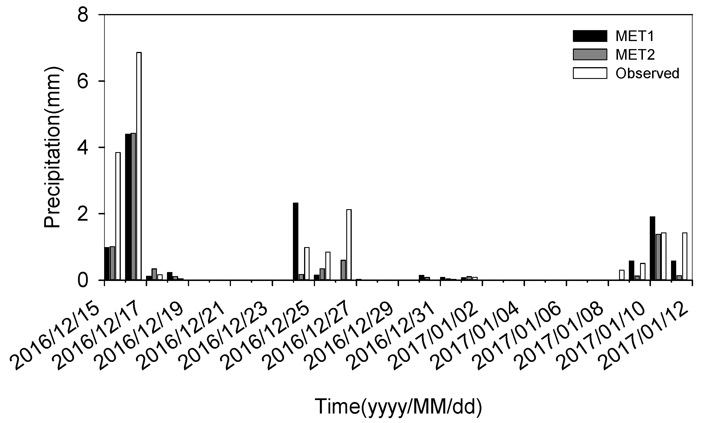
3.1. Evaluation of Meteorology

Meteorological conditions are very important for pollution accumulation and diffusion and can contribute to 2/3 of the causes of heavy pollutions [54]. Studies have shown that elements like wind speed, temperature and humidity are more difficult to simulate correctly in the near surface layer than at the high level even though they are more important for pollutant variation [25]. Therefore, the evaluation of this study focuses mostly on the near-surface meteorological elements (Table 3 and Table 4).
MET1 and MET2 show good simulation results for the 2 m temperature, with the correlation coefficients both reaching 0.83 and RMSE being less than 2 °C (Table 3). The 2 m temperature are slightly overestimated by MET1 but slightly underestimated by MET2. RMSE is slightly less in MET1 than that in MET2.
The correlation coefficient of both MET1 and MET2 are not high, which reflects the complexity of the boundary layer wind speed simulation (Table 4). The RMSE in MET2 is much lower than that of MET1, indicating a better ability of MET2 to simulate low wind speed in static weather.
The simulation accuracy of temperature and wind speed in this study is close to or better than that of similar research results. For example, Ning et al. once used WRF/Chem to simulate a winter pollution episode in Chengdu, and their results demonstrated that the correlation coefficients between the simulation and observation of 2 m temperature and 10 m wind speed were 0.75 and 0.22, respectively, and the mean of 10 m wind speed simulation was significantly higher than the observed value [55]. Several researchers have also found that the near-surface wind speeds by WRF/Chem are generally overestimated [56,57,58,59].
Because the relative humidity is very important for the hygroscopic growth of aerosols [60,61], we compared the simulation and observation results of relative humidity (Figure 2). The results show that: observation > MET2 > MET1. The change trend in the three curves is relatively consistent, but the observed values are higher regardless of the peak or valley. Especially near 27 December 2016 (corresponding to the low pollutant concentrations), the relative humidity of MET1 and MET2 is below 50%, while the observed value is above 60%.
The lower planetary boundary layer height (PBLH) is more beneficial to the accumulation of pollutants, promoting the formation of heavy pollution. Therefore, the PBLH is also an important parameter for the static condition of the near-surface atmosphere. Due to the lack of observational data, it is difficult to obtain accurate PBLH observations. Previous studies show that PBLH is generally less than 1 km during heavy pollution in the Sichuan Basin using the fine-resolution sounding measurements from 2014 to 2017 [62]. It shows that PBLH by MET2 is mostly near or less than 1 km and obviously lower than that by MET1, which is larger than 1 km during the two episodes (Figure 3). Therefore, the result for MET2 is closer to the actual boundary layer height during a heavy-pollution period than the result of MET1. It also shows that the diurnal variations of PBLH in both MET1 and MET2. This is because of the arbitrary regime division of the unstable and stable PBL schemes in meteorological models [25].
To sum up, both MET1 and MET2 can simulate the static weather pattern, while MET2 is a little superior to MET1 in terms of near-surface low wind speed and low PBLH.

3.2. Episodes Evaluation

Figure 4 shows the simulated and observed PM2.5 and PM10 concentrations averaged from the selected five cities in Southern Sichuan, and the simulated and observed ratios of PM2.5 in PM10 during the two pollution episodes. The simulated PM2.5 concentration is averaged for the four tests and the five cities. According to the observation, the life cycle of the start, maintenance and end of the two pollution episodes are very obvious, during which the peak values of PM2.5 are 156.2 μg m3 and 197.4 μg m3, and the peak values of PM10 are 200.4 μg m3 and 247.4 μg m3, respectively. During the two episodes, the ratio of PM2.5 in PM10 is generally more than 70% except in the pollution transition period in which the value drops to near 55%, which demonstrates that finer particles are the main particulate pollutant during the polluted episodes. The simulated results also show the life cycles of the start, development and dissipation of the two pollution events (Figure 4). The simulated peak concentrations of pollutants are relatively higher than the observed values, and the proportions of PM2.5 in PM10 remain stable at more than 90%, obviously higher than the observed values. This suggests that the model can simulated the pollution episodes in terms of the life circle but it still has bias for the variations during the maintaining period and for the coarse particles with diameter between 2.5 μm and 10 μm.
Here we compare the time series of observed and simulated PM2.5 concentrations of the five cities for each individual test (Figure 5). It shows that each test has good capability for the simulation of life cycle these two episodes. The simulation results also reflect well the start and end times of the two heavy pollution episodes and the changing trend of PM2.5 concentration growth, accumulation and dissipation of all the four tests. It also shows that the variation trends of PM2.5 shown by the four schemes are very agreed.
In the Pollution Episode I the observed PM2.5 concentration presents the pattern of rising, slightly falling, rising again (not exceeding the first peak), and then falling again till the end of the pollution episode, but the simulation shows the pattern of rising, daily fluctuating slightly, and falling rapidly to the end of the pollution episode. It has not so monotonous increase and decrease as the observed. For the Pollution Episode II, the observed PM2.5 concentration rises and then fluctuates down till the end of the pollution episode, while the simulation results show that it rises, clearly descends for a relative long time, then rises again (slightly higher than the previous peak) and finally rapidly goes to the end of the pollution episode, still having not so clearly momentous increase and decrease as the observed.
By analyzing the precipitation(Figure 6), we found that the long-time descending during the Pollution Episode II is due to the abnormal precipitation from the model, whose result shows that MET1 and MET2 both predicted the precipitation during the long-time descending at all five stations. During the period from 31 December 2016 to 1 January 2017 (Figure 7), the simulated precipitation of MET1 and MET2 is higher than the observation. In these three days, the simulation results show that it rains every day, but the observation is only two days, and the observed rainfall is smaller. This shows that the simulated precipitation is much more and the duration is much longer. Therefore, the underestimation of PM2.5 in the continuous phase of Pollution Episode II is mainly caused by the large abnormal wet removal. On the other hand, the smaller rainfall can not effectively clear the pollutants, and the pollution is still serious after the rainfall.

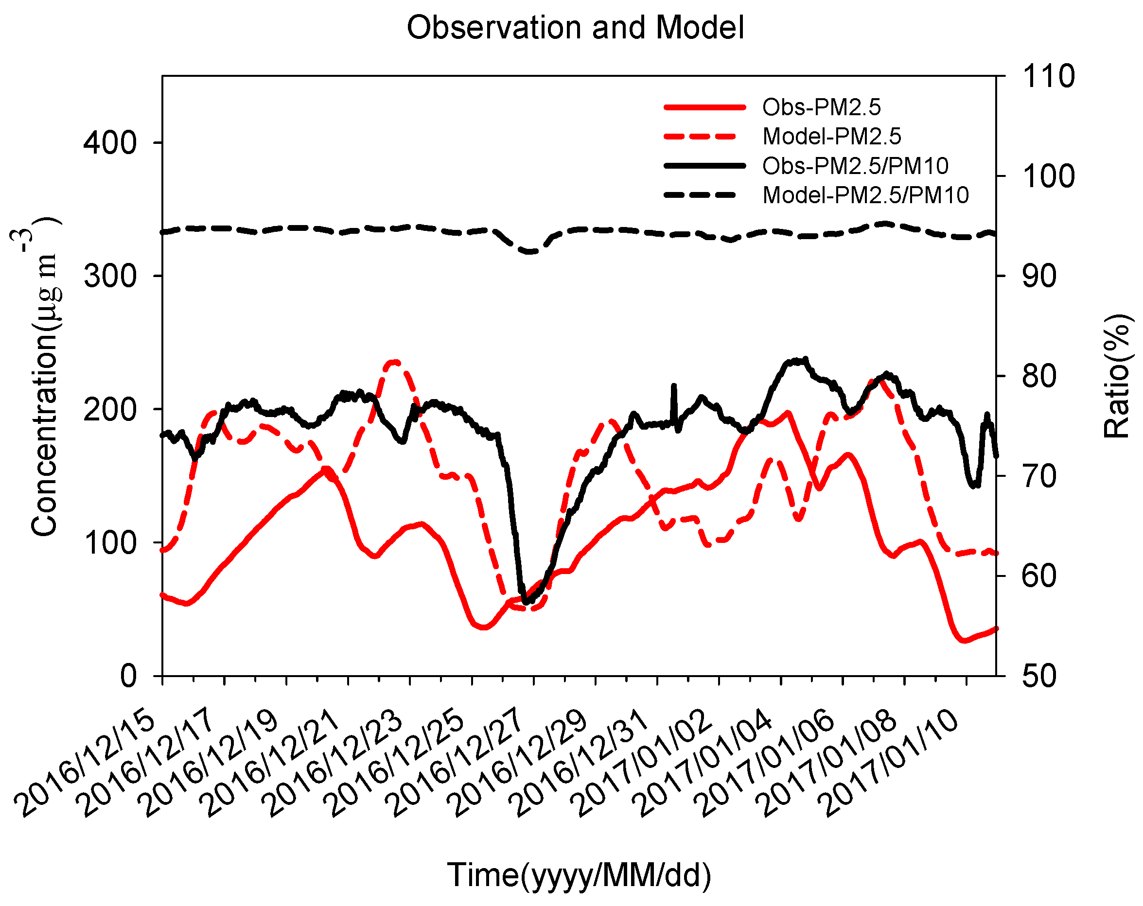
3.3. PM2.5 Evaluation

The statistical analyses of the two pollution episodes in the four tests are given in Table 5 and Table 6. Except for the average value of CUACE-MET1 in the Pollution Episode II, which is slightly smaller and very close to the observed value, the mean PM2.5 concentrations of the other three are obviously larger than the observed value. In the both processes, the correlation coefficient of MET2s with the same chemical processes is higher than that of MET1s, and the correlation coefficient of CUACEs with the same meteorological processes is higher than that of Chems. The correlation coefficients of each test in the Pollution Episode I are above 0.4, with the highest reaching 0.48 in CUACE-MET2, and the correlation is better than that of the Pollution episode II. The RMSE of MET1s in both processes is apparently smaller than that of MET2s, and of CUACEs is greatly smaller than that of Chems. In the study by James W. et al. [63], it has been proposed that a model performance goal has been met when both the mean fractional error (MFE) and the mean fractional bias (MFB) are less than or equal to +50% and ±30%, respectively. Additionally, the model performance criteria has been met when both the MFE ≤ +75% and MFB ≤ ±60%. In the Pollution Episode I, only CUACE-MET1 had MFE less than 50% and MFB less than 30%. The MFE and MFB of the four groups of experiments were all less than 75% and 60%, respectively. In the Pollution Episode II, the MFE and MFB of the four groups of experiments were all less than 50% and 30%, respectively.
It can be seen from the above simulation results that CUACE performs better than Chem interns of both correlation coefficients and RMSE. The analysis results of Section 3.1 show that MET2 performs better for static weather than that of MET1. But for the point of PM2.5 concentration, the two schemes have no clear superiority for one or another. This reveals again that the complex interactions between the meteorology and pollution.

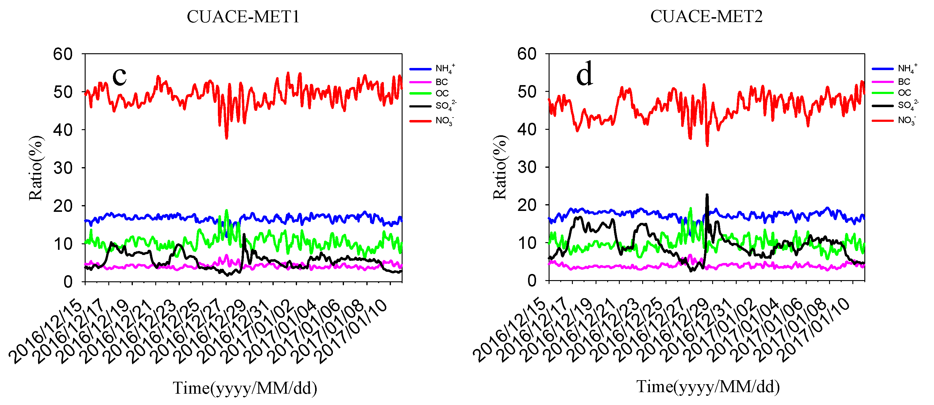
3.4. Aerosol Component Evaluation

We also analysis the temporal variations of different aerosol components in each test (Figure 8). It indicates that the time variation of each component is very consistent with the time variation of PM2.5 in Figure 5. The results again denote that the main factors affecting the quick changes of aerosol components are the changing meteorological conditions in short time period. Both in the time series of Figure 4 and Figure 5 and the statistics results in Table 5 and Table 6 shows the highly overestimated concentration of PM2.5 simulated. In Figure 8, we see the obviously high concentrations of nitrate in all the four tests. The concentration proportion of each component also shows this phenomenon, the proportion of nitrate is the highest, fluctuating between 40% and 50% in all of the four groups of tests (Figure 9). The ratios of ammonium is accounting for 15–18%. The ratio of OC is between 8% and 18%, and the minimum proportion is BC, around 5%. The average proportion of sulfates is 7.5%. These results of sulfate, OC and BC are consistent with the observations from Atmospheric Research Laboratory of Chengdu Academy of Environmental Sciences, and National Air Pollution Control and Associated Center, which means that ammonium accounts for 20–23%, BC 3%, OC 11–12%, sulfate 7–8%. But for nitrate, the observation only accounts for 27–33%, with very scarcely value reaching 40% which indicates that nitrate is clearly overestimated. This is consistent with the unified overestimations of nitrate in China in Miao et al.’s work [64].

3.5. Potential Contributors to the Abnormally High Nitrate Concentration

Nitrate is thermodynamically unstable, whose concentration is affected by multiple elements like atmospheric conditions, concentrations of precursors, sulfate and nitrate, etc. Therefore, we also analyze its relations among nitrate, sulfate and ammonium (Table 7 and Table 8).
Table 7 illustrates significant positive correlations among nitrate, sulfate and ammonium in all the four tests. This is consistent with the results of Section 3.3 and again explains that the change of components is mainly controlled by the change of meteorological elements. The correlation among the ratios of the three components in PM2.5 is further analyzed to exclude the influence of meteorological factors (Table 8). The concentration ratios of nitrate and sulfate are negatively correlated, but those of sulfate and ammonium, nitrate and ammonium are all obviously positively correlated. Sulfate, nitrate, and ammonium exist thermodynamically in the form of ammonium sulfate and ammonium nitrate in the atmosphere, so sulfate and nitrate have to compete to get ammonium which is depicted by their negative correlations in Table 8. Nitrate and sulfate in Chems is poorly correlated with the value of 0.09 and −0.13 in Chem-MET1 and Chem-MET2, indicating that Chem is insufficient for the competition mechanism of nitrate and sulfate. The correlation between nitrate and sulfate in CUACE is −0.20 (CUACE-MET1) and −0.55 (CUACE-MET2) respectively. This shows that CUACE pays more attention to the competitive mechanism of nitrate and sulfate. CUACE-MET2 > CUACE-MET1 also shows that different meteorological processes will affect the reaction and transformation between chemical substances. For the correlation between nitrate and ammonium, the experimental result shows that Chem-MET1 > Chem-MET2 > CUACE-MET1 > CUACE-MET2. For the correlation between sulfate and ammonium, the experimental results show that Chem-MET1 ≈ Chem-MET2 < CUACE-MET1 < CUACE-MET2, is contrary to the order of correlation between nitrate and ammonium in the four groups. The two chemical models are much more stable for sulfate ammonium simulation, among which the CUACE correlation is better.
NO2 and SO2 are the precursor materials of sulfate and nitrate production, and their concentration changes have a great impact on the concentration of sulfate and sulfate in the atmosphere [22]. Therefore, we also analyzed the concentration of NO2 and SO2. The concentration of NO2 in the four tests is obviously lower than the observed ones, indicating that the model overestimates the conversion of NO2 to nitrate which is the cause of the high nitrate concentrations (Figure 10a). Comparatively, the simulation results of SO2 in the four groups are higher than those observed, but the simulated sulfate is lower (average proportion is 7.5%), which suggests that the model have still underestimated the conversion of SO2 to sulfate (Figure 10b).
This is also true in statistical results in Table 9. It can be seen that nitrate and NO2 are negatively correlated while sulfate and SO2 are positively correlated in the four tests. It also shows that more NO2 is converted into nitrate and less left to be accumulated, while some SO2 can still accumulate and other convert into sulfate in heavy pollution condition. The negative correlation between nitrate and NO2 is more noticeable in CUACE than in Chem, in MET2 than in MET1, so for the positive correlations. Hence, the conversion relationship between CUACE’s sulfate and nitrate and their precursors is more reasonable.
We analyzed the correlation of ammonia(NH3), nitric acid(HNO3), 2m temperature(T2) and relative humidity(RH). The results(Table 10) showed that NH3 was generally positively correlated with RH and negatively correlated with T2. On the contrary, HNO3 is negatively correlated with RH and positively correlated with T2. The general negative correlation between ammonia and nitric acid is consistent with the fact that they react to form ammonium nitrate.
The results of the four experiments show that each correlation coefficient of Chem-MET1 is the largest among the four experiments. This shows that Chem-MET1 pays the most attention to the correlation between these factors. For the two groups of experiments using MET2, whether Chem or CUACE, the experimental results are relatively similar, and the correlation coefficient is small. By comparing the two groups of experiments using MET1, we found that CUACE and Chem had the same results for the correlation between NH3 and meteorological elements, but there was a significant gap between CUACE and Chem for the correlation between HNO3 and meteorological elements. This shows that the influence of meteorological elements on nitric acid in Chem is more obvious.

4. Summary and Conclusions

The online air quality models WRF/Chem and WRF/CUACE have been used to simulate the two heavy pollution episodes in one month that occurred in the Southern Sichuan basin, one of the four major pollution zones in China, from 15 December 2016 to 11 January 2017. The driving weather model WRF has a good simulation effect of 2 m temperature in Southern Sichuan, which is close to the observation with good correlation coefficient and small error. It can also simulate well the low wind speed and boundary layer height, which are important variables of static weather, providing a good meteorological background for model to simulate pollution episodes.
Both Chem and CUACE have accurately simulated the life cycle of the two pollution events in terms of the onset, maintenance and dissipating phase. In the four tests, the variation trends of the PM2.5 concentration, which is an important indicator of haze-fog, and the concentration of each component are in line with the development of pollution episode. The proportion of each component in PM2.5 is very close to the observation except the extraordinary overestimated nitrate. The overestimation of nitrate has been pinned down in this paper and it is due to the model overestimation of the conversion of NO2 to nitrate and underestimations of the conversion of SO2 to sulfate.
Meteorological parameterizations all have important impacts on the model simulation results. MET2 can simulate stronger atmospheric static weather conditions than MET1 dose. It also shows a relatively better performance than MET1 in terms of higher correlation coefficients and lower errors in most of the particles and particulate components evaluations. CUACE also shows a relatively better performance in terms of higher correlation coefficients and lower errors in most of the particles and particulate components evaluations. It also performs better in the competitive mechanism of sulfate and nitrate against ammonium in the thermodynamic equilibrium mechanism. However, the negative correlation between the two is not obvious in the results of Chem model. Then, CUACE-MET2 performs the best in all the four tests.
The static weather is very important condition for pollutants to be accumulated and is also the most complex and difficult weather conditions to be accurately simulated due to the models limitation in the near surface of the atmosphere. More light should shine into this hard core of pollutions. And nitrate is the main source of deviations in aerosol simulation at present in many air pollutions models. With the increase of the national emission reduction mechanism in China, the proportion of nitrate in particulate matters is getting higher and higher and will be the major component in particles in the near future. The mechanism of mutual conversion between nitrate and other components also need more detail research together with more comprehensive observations.

Author Contributions

Conceptualization, L.C. and C.Z.; methodology, L.C. and C.Z.; software, L.C. and L.Z.; validation, L.C., C.Z. and L.Z.; formal analysis, L.C. and C.Z.; investigation, L.C.; resources, C.Z.; data curation, L.C. and L.Z.; writing—original draft preparation, L.C.; writing—review and editing, L.C. and C.Z.; visualization, L.C.; supervision, C.Z. and S.W.; project administration, C.Z. and S.W.; funding acquisition, C.Z. and S.W. All authors have read and agreed to the published version of the manuscript.

Funding

This research was funded by the National Key Project of the Ministry of Science and Technology of China(2022YFC3700303); CMA Innovation Development Project (CXFZ2021J023). And the APC was funded by the National Key Project of the Ministry of Science and Technology of China(2022YFC3700303); CMA Innovation Development Project (CXFZ2021J023).

Acknowledgments

The meteorological initial and boundary conditions for the modeling system were obtained from the China Meteorological Data Sharing Service System (http://data.cma.cn/data/cdcindex/cid/98c64da7ee348b37.html). The meteorological observations were obtained from the China Meteorological Data Sharing Service System (http://data.cma.cn/data/cdcindex/cid/f0fb4b55508804ca.html).

Conflicts of Interest

The authors declare no conflict of interest.

References

  1. Chen, Y.; Xie, S. Temporal and spatial visibility trends in the Sichuan Basin, China, 1973 to 2010. Atmos. Res. 2012, 112, 25–34. [Google Scholar] [CrossRef]
  2. Qiao, X.; Jaffe, S.; Tang, Y.; Bresnahan, M.; Song, J. Evaluation of air quality in Chengdu, Sichuan Basin, China: Are China’s air quality standards sufficient yet? Environ. Monit. Assess. 2015, 187, 1–11. [Google Scholar] [CrossRef] [PubMed]
  3. Liu, X.; Chen, Q.; Che, H.; Zhang, R.; Gui, K.; Zhang, H. Spatial distribution and temporal variation of aerosol optical depth in the Sichuan basin, China, the recent ten years. Atmos. Environ. 2016, 147, 434–445. [Google Scholar] [CrossRef]
  4. Wang, L.; Stanič, S.; Bergant, K.; Eichinger, W.; Močnik, G.; Drinovec, L.; Vaupotič, J.; Miler, M.; Gosar, M.; Gregoric, A. Retrieval of vertical mass concentration distributions—Vipava valley case study. Remote Sens. 2019, 11, 106. [Google Scholar] [CrossRef] [Green Version]
  5. Wang, L.; Mačak, M.B.; Stanič, S.; Bergant, K.; Gregorič, A.; Drinovec, L. Investigation of Aerosol Types and Vertical Distributions Using Polarization Raman Lidar over Vipava Valley. Remote Sens. 2022, 14, 3482. [Google Scholar] [CrossRef]
  6. Zhang, X. Characteristics of the chemical components of aerosol particles in the various regions over China. Acta Meteorol. Sin. 2014, 72, 1108–1117. [Google Scholar]
  7. Zhang, Y.; Tian, Q.Q.; Wei, X.Y.; Zhang, S.B.; Hu, W.D.; Li, M.G. Health Benefit Evaluation for PM2.5 as Well as O3-8h Pollution Control in Chengdu, China from 2016 to 2020. Environ. Sci. 2022, 1–16. [Google Scholar] [CrossRef]
  8. Chen, K.; Wang, Z.; Liu, Z.; Huang, G.; Xiang, Q. The temporal evolvement characteristics of air pollution of the urban agglomeration in Southern Sichuan from 2005 to 2014. Environ. Eng. 2017, 35, 72–76, 81. [Google Scholar]
  9. Zhang, J.; Liu, Z.; Huang, G.; He, M. The spatial and temporal distribution and meteorological factor analysis of air pollution of the urban agglomeration in Southern Sichuan. Sichuan Environ. 2017, 36, 69–75. [Google Scholar]
  10. Zhao, S.; Yu, Y.; Yin, D.; Qin, D.; He, J.; Dong, L. Spatial patterns and temporal variations of six criteria air pollutants during 2015 to 2017 in the city clusters of Sichuan Basin, China. Sci. Total Environ. 2018, 624, 540–557. [Google Scholar] [CrossRef]
  11. Lin, N. The Research on Transport Law of Atmospheric Pollutant and Joint Prevention and Control of Air Pollution Technology in Sichan Province. Master’s Thesis, Southwest Jiaotong University, Chengdu, China, 2015. [Google Scholar]
  12. Wang, L.; Xiang, W.; Chen, Y.; Xiao, T.A. Continuous pollution episode analysis in south of Sichuan urban agglomeration. J. Chengdu Univ. Inf. Technol. 2017, 32, 214–219. [Google Scholar]
  13. He, M.; Liu, Z.; Zhang, Y.; Zhang, Y.; Yan, Y.; Huang, G. Analyses on the spatial-temporal distribution features and causing factors of atmospheric haze in the southern city-group of Sichuan. China Environ. Sci. 2017, 37, 432–442. [Google Scholar]
  14. Zhang, Y. Online-coupled meteorology and chemistry models: History, current status, and outlook. Atmos. Chem. Phys. 2008, 8, 2895–2932. [Google Scholar] [CrossRef] [Green Version]
  15. Qin, S. Numerical Simulation Study of PM2. 5 Pollution in Fushun City Based on the WRF-CMAQ Model. Environ. Prot. Sci. 2018, 44, 80–84. [Google Scholar]
  16. Xiong, Y.; Xu, J.; Sun, Z.; Li, Z.; Wu, J.; Yin, X. Air pollution reduction effect evaluation based on data mining algorithm and numerical simulation technology. Acta Sci. Circumstantiate 2019, 39, 116–125. [Google Scholar]
  17. Fu, Y.; Li, H.; Yu, H.; Wang, X.; Zhao, F.; Zhou, D. Weather characteristics and simulation analysis on causes of air pollution in Dalian. China Environ. Sci. 2018, 38, 3639–3646. [Google Scholar]
  18. Tie, X.; Geng, F.; Peng, L.; Gao, W.; Zhao, C. Measurement and modeling of O3 variability in Shanghai, China: Application of the WRF-Chem model. Atmos. Environ. 2009, 43, 4289–4302. [Google Scholar] [CrossRef]
  19. Zhang, L.; Zhu, B.; Gao, J.; Kang, H.Q.; Yang, P.; Wang, H.L.; Li, Y.E.; Shao, P. Modeling Study of a Typical Summer Ozone Pollution Event over Yangtze River Delta. Environ. Sci. 2015, 36, 3981–3988. [Google Scholar]
  20. Chen, X.R.; Wang, H.C.; Lu, K.D. Simulation of organic nitrates in Pearl River Delta in 2006 and the chemical impact on ozone production. Sci. China 2018, 61, 228–238. [Google Scholar] [CrossRef]
  21. Fan, Q.; Lan, J.; Liu, Y.; Wang, X.; Chan, P.; Hong, Y.; Feng, Y.; Liu, Y.; Zeng, Y.; Liang, G. Process analysis of regional aerosol pollution during spring in the Pearl River Delta region, China. Atmos. Environ. 2015, 122, 829–838. [Google Scholar] [CrossRef]
  22. Wang, W.; Liu, M.; Wang, T.; Song, Y.; Zhou, L.; Cao, J.; Hu, J.; Tang, G.; Chen, Z.; Li, Z.; et al. Sulfate formation is dominated by manganese-catalyzed oxidation of SO2 on aerosol surfaces during haze events. Nat. Commun. 2021, 12, 1–10. [Google Scholar] [CrossRef] [PubMed]
  23. Zhao, X.; Xu, J.; Zhang, Z.; Zhang, X.; Fan, S.; Su, J. Beijing Regional Environmental Meteorology Prediction System and Its Performance Test of PM2.5 Concentration. J. Appl. Meteorol. Sci. 2016, 27, 160–172. [Google Scholar]
  24. Zhou, C.H.; Gong, S.L.; Zhang, X.Y.; Wang, Y.Q.; Niu, T.; Liu, H.L. Development and evaluation of an operational SDS forecasting system for East Asia: CUACE/Dust. Atmos. Chem. Phys. 2008, 8, 787–798. [Google Scholar] [CrossRef] [Green Version]
  25. Zhou, C.H.; Gong, S.L.; Zhang, X.Y.; Liu, H.L.; Xue, M.; Cao, G.L. Towards the improvements of simulating the chemical and optical properties of Chinese aerosols using an online coupled model—CUACE/Aero. Tellus B Chem. Phys. Meteorol. 2012, 64, 18965. [Google Scholar] [CrossRef] [Green Version]
  26. Zhou, C.H. On-Line Numerical Research on Atmospheric Aerosols and Their Interaction with Clouds and Precipitation. Ph.D. Thesis, University of Chinese Academy of Sciences, Beijing, China, 2013. [Google Scholar]
  27. Grell, G.A.; Peckham, S.E.; Schmitz, R.; McKeen, S.A.; Frost, G.; Skamarock, W.C.; Eder, B. Fully coupled “online” chemistry within the WRF model. Atmos. Environ. 2005, 39, 6957–6976. [Google Scholar] [CrossRef]
  28. Zhang, L.; Gong, S.L.; Zhao, T.L.; Zhou, C.H.; Wang, Y.S.; Li, J.W.; Ji, D.S.; He, J.J.; Liu, H.L.; Gui, K.; et al. Development of WRF/CUACE v1.0 model and its preliminary application in simulating air quality in China. Geosci. Model Dev. 2021, 14, 703–718. [Google Scholar] [CrossRef]
  29. Nenes, A.; Pilinis, C.; Pandis, S.N. ISORROPIA: A New Thermodynamic Equilibrium Model for Multiphase Multicomponent Inorganic Aerosols. Aquat. Geochem. 1998, 4, 123–152. [Google Scholar] [CrossRef]
  30. Nenes, A.; Pandis, S.N.; Pilinis, C. Continued development and testing of a new thermodynamic aerosol module for urban and regional air quality models. Atmos. Environ. 1999, 33, 1553–1560. [Google Scholar] [CrossRef]
  31. Petroff, A.; Zhang, L. Development and validation of a size-resolved particle dry deposition scheme for application in aerosol transport models. Geosci. Model Dev. 2010, 3, 753–769. [Google Scholar] [CrossRef] [Green Version]
  32. Gong, S.L.; Barrie, L.A.; Salzen, K.; Lohmann, U.; Lesins, G.; Spacek, L.; Zhang, L.; Girard, E.; Lin, H.; Leaitch, R.; et al. Canadian Aerosol Module: A size-segregated simulation of atmospheric aerosol processes for climate and air quality models 1. Module development. J. Geophys. Res. 2003, 108, 4007. [Google Scholar] [CrossRef]
  33. Zhang, L. Influences of Atmospheric Particle Source-Sink Processes on Air Quality Change in China: Coupling Atmospheric Chemistry Model WRF-CUACE and Modeling Experiments. Ph.D. Thesis, Nanjing University of Information Engineering, Nanjing, China, 2019. [Google Scholar]
  34. Lin, Y.-L.; Farley, R.D.; Orville, H.D. Bulk Parameterization of the Snow Field in a Cloud Model. J. Clim. Appl. Meteorol. 1983, 22, 1065–1092. [Google Scholar] [CrossRef]
  35. Mlawer, E.J.; Taubman, S.J.; Brown, P.; Iacono, M.J.; Clough, S. Radiative transfer for inhomogeneous atmosphere: RRTM. J. Geophys. Res. D Atmos. 1997, 102, 16663–16682. [Google Scholar] [CrossRef] [Green Version]
  36. Chou, M.-D.; Suarez, M.J.; Ho, C.-H.; Yan, K.-T. Parameterizations for Cloud Overlapping and Shortwave Single-Scattering Properties for Use in General Circulation and Cloud Ensemble Models. J. Clim. 1998, 11, 202–214. [Google Scholar] [CrossRef]
  37. Janjić, Z.I. The Step-Mountain Eta Coordinate Model: Further Developments of the Convection, Viscous Sublayer, and Turbulence Closure Schemes. Mon. Weather. Rev. 1994, 122, 927–945. [Google Scholar] [CrossRef]
  38. Zilitinkevich, S. Non-local turbulent transport: Pollution dispersion aspects of coherent structure of connective flows. Trans. Ecol. Environ. 1995, 6, 53–60. [Google Scholar]
  39. Chen, F.; Dudhia, J. Coupling an Advanced Land Surface–Hydrology Model with the Penn State–NCAR MM5 Modeling System. Part I: Model Implementation and Sensitivity. Mon. Weather. Rev. 2001, 129, 569–585. [Google Scholar] [CrossRef]
  40. Wang, H. Radiative feedback of dust aerosols on the East Asian dust storms. J. Geophys. Res. 2010, 115, 13430. [Google Scholar] [CrossRef]
  41. Xiao, D.; Chen, J.; Chen, Z.; Zhang, B. Effect simulation of Chengdu fine underlying surface information on urban meteorology. Meteorol. Mon. 2011, 37, 298–308. [Google Scholar]
  42. Zeng, X.M.; Wang, B.; Zhang, Y.; Song, S.; Huang, X.; Zheng, Y. Sensitivity of high-temperature weather to initial soil moisture: A case study with the WRF model. Atmos. Chem. Phys. Discuss. 2014, 14, 11665–11714. [Google Scholar] [CrossRef] [Green Version]
  43. Santos-Alamillos, F.J.; Pozo-Vázquez, D.; Ruiz-Arias, J.A.; Lara-Fanego, V.; Tovar-Pescador, J. Analysis of WRF Model Wind Estimate Sensitivity to Physics Parameterization Choice and Terrain Representation in Andalusia (Southern Spain). J. Appl. Meteorol. Climatol. 2013, 52, 1592–1609. [Google Scholar] [CrossRef]
  44. Zhu, K.; Xue, M. Evaluation of WRF-based convection-permitting multi-physics ensemble forecasts over China for an extreme rainfall event on 21 July 2012 in Beijing. Adv. Atmos. Sci. 2016, 33, 1240–1258. [Google Scholar] [CrossRef]
  45. Morrison, H.; Thompson, G.; Tatarskii, V. Impact of Cloud Microphysics on the Development of Trailing Stratiform Precipitation in a Simulated Squall Line: Comparison of One- and Two-Moment Schemes. Mon. Weather. Rev. 2009, 137, 991–1007. [Google Scholar]
  46. Iacono, M.J.; Delamere, J.S.; Mlawer, E.J.; Shephard, M.W.; Clough, S.A.; Collins, D.W. Radiative Forcing by Long-Lived Greenhouse Gases: Calculations with the AER Radiative Transfer Models. J. Geophys. Res. Atmos. 2008, 113, 1–22. [Google Scholar] [CrossRef]
  47. Dudhia, J. Numerical Study of Convection Observed during the Winter Monsoon Exiperiment Using a Mesoscale Two-Dimensional Model. J. Atmos. Sci. 1989, 46, 3077–3107. [Google Scholar]
  48. Zaveri, R.A.; Easter, R.C.; Fast, J.D.; Peters, L.K. Model for Simulating Aerosol Interactions and Chemistry (MOSAIC). J. Geophys. Res. 2008, 113, 1–29. [Google Scholar] [CrossRef]
  49. Zaveri, R.A.; Peters, L.K. A new lumped structure photochemical mechanism for large-scale applications. J. Geophys. Res. Atmos. 1999, 104, 30387–30415. [Google Scholar] [CrossRef]
  50. Stockwell, W.R.; Middleton, P.; Chang, J.S. The Second Generation Regional Acid Deposition Model Chemical Mechanism for Regional Air Quality Modeling. J. Geophys. Res. 1990, 95, 16343–16367. [Google Scholar] [CrossRef]
  51. Stockwell, W.R.; Kirchner, F.; Kuhn, M.; Seefeld, S. A new mechanism for regional atmospheric chemistry modeling. J. Geophys. Res. Atmos. 1997, 102, 25847–25879. [Google Scholar]
  52. Li, M.; Zhang, Q.; Kurokawa, J.-I.; Woo, J.-H.; He, K.; Lu, Z.; Ohara, T.; Song, Y.; Streets, D.G.; Carmichael, G.R.; et al. MIX: A mosaic Asian anthropogenic emission inventory under the international collaboration framework of the MICS-Asia and HTAP. Atmos. Chem. Phys. 2017, 17, 935–963. [Google Scholar] [CrossRef] [Green Version]
  53. Zhang, L.; Zhao, T.; Gong, S.; Kong, S.; Tang, L.; Liu, D. Updated emission inventories of power plants in simulating air quality during haze periods over East China. Atmos. Chem. Phys. 2018, 18, 2065–2079. [Google Scholar]
  54. RenHe, Z.; Li, Q.; Zhang, R. Meteorological conditions for the persistent severe fog and haze event over eastern China in January 2013. Sci. China Earth Sci. 2013, 57, 26–35. [Google Scholar] [CrossRef]
  55. Ning, G. Meteorological Causes of Air Pollution in the Northwest Urban Agglomeration of Sichuan Basin in Winter and Their Numerical Simulation. Master’s Thesis, Meterology, Lanzhou University, Lanzhou, China, 2017. [Google Scholar]
  56. Tuccella, P.; Curci, G.; Visconti, G.; Bessagnet, B.; Menut, L.; Park, R.J. Modeling of gas and aerosol with WRF/Chem over Europe: Evaluation and sensitivity study. J. Geophys. Res. Atmos. 2012, 117. [Google Scholar] [CrossRef] [Green Version]
  57. Liao, L.; Liao, H. Role of the radiative effect of black carbon in simulated PM2.5 concentrations during a haze event in China. Atmos. Ocean. Sci. Lett. 2017, 7, 434–440. [Google Scholar] [CrossRef]
  58. Wang, L.; Zhang, Y.; Wang, K.; Zheng, B.; Zhang, Q.; Wei, W. Application of Weather Research and Forecasting Model with Chemistry (WRF/Chem) over northern China: Sensitivity study, comparative evaluation, and policy implications. Atmos. Environ. 2016, 124, 337–350. [Google Scholar] [CrossRef] [Green Version]
  59. Yu, Y.; Liao, L.; Cui, X.; Chen, F. Effects of different anthropogenic emission inventories on simulated air pollutants concentrations: A case study in Zhejiang Province. Clim. Environ. Res. 2017, 22, 519–537. [Google Scholar]
  60. Cheng, Y.; He, K.B.; Du, Z.Y.; Zheng, M.; Duan, F.K.; Ma, Y.L. Humidity plays an important role in the PM2.5 pollution in Beijing. Environ. Pollut. 2015, 197, 68–75. [Google Scholar] [CrossRef]
  61. Carrico, C.M.; Kreidenweis, S.M.; Malm, W.C.; Day, D.E.; Lee, T.; Carrillo, J. Hygroscopic growth behavior of a carbon-dominated aerosol in yosemite national park. Atmos. Environ. 2005, 39, 1393–1404. [Google Scholar] [CrossRef]
  62. Miao, Y.; Liu, S.; Guo, J.; Huang, S.; Yan, Y.; Lou, M. Unraveling the relationships between boundary layer height and PM2.5 pollution in China based on four-year radiosonde measurements. Environ. Pollut. 2018, 243, 1186–1195. [Google Scholar] [CrossRef]
  63. Boylan, J.W.; Russell, A.G. Pm and light extinction model performance metrics, goals, and criteria for three-dimensional air quality models. Atmos. Environ. 2006, 40, 4946–4959. [Google Scholar] [CrossRef]
  64. Miao, R.; Chen, Q.; Zheng, Y.; Cheng, X.; Sun, Y.; Palmer, P.I.; Shrivastava, M.; Guo, J.; Zhang, Q.; Liu, Y.; et al. Model bias in simulating major chemical components of PM2.5 in China. Atmos. Chem. Phys. 2020, 20, 12265–12284. [Google Scholar] [CrossRef]
Figure 1. Distribution diagram of simulation area settings (D1: Domain 1; D2: Domain 2; D3: Domain 3; The shaded map is for terrain height from sea level); D3 also includes the locations of Chengdu, Leshan, Luzhou, Neijiang, Yibin and Zigong.
Atmosphere 13 01771 g001
Figure 2. Time series of relative humidity (RH, unit: %) in simulation results of MET1 (black solid line), MET2 (grey dot dash line) and Observed (black dash line).
Atmosphere 13 01771 g002
Figure 3. Time series of boundary layer height (PBLH, unit: m) in simulation results of MET1 (black solid line) and MET2 (red solid line).
Atmosphere 13 01771 g003
Figure 4. Time series of simulated and observed hourly mean PM2.5 concentrations (μg m−3) and ration of PM2.5 in PM10 (unit:%) of the five cities in Southern Sichuan from 15 December 2016 to 11 January 2017. The solid black line is for Obs-PM2.5, the dash black line is for the ratio of observed PM2.5 in PM10. The solid red line is for Model-PM2.5, the dash red line is for the ratio of simulated PM2.5 in PM10.
Atmosphere 13 01771 g004
Figure 5. Time series of hourly the 24 h averages of the observed PM2.5 concentration (unit: μg m−3) from 15 December 2016 to 11 January 2017 (solid black line) and simulated PM2.5 concentration from the four groups of tests (red dotted line: Chem-MET1; red solid line: Chem-MET2; blue dotted line: CUACE-MET1; blue solid line: CUACE-MET2) (unit: μg m−3).
Atmosphere 13 01771 g005
Figure 6. Histogram of hourly the 24 h averages of the observed precipitation (unit: mm) from 15 December 2016 to 11 January 2017 (white bar) and simulated precipitation of MET1 (black bar) and MET2 (grey bar).
Atmosphere 13 01771 g006
Figure 7. Histogram of hourly the 24 h averages of the observed precipitation (unit: mm) from 29 December 2016 to 02 January 2017 (white bar) and simulated precipitation of MET1 (black bar) and MET2 (grey bar).
Atmosphere 13 01771 g007
Figure 8. Time series of daily averages of the concentrations of ammonium (blue solid line), BC (purple solid line), OC (green solid line), sulfate (blue solid line), and nitrate (red solid line) by Chem-MET1 (a), Chem-MET2 (b), CUACE-MET1 (c) and CUACE-MET2 (d) (unit: μg m−3).
Atmosphere 13 01771 g008
Figure 9. Hourly time series of concentration ratios of ion ammonium salt (blue solid line), BC (purple solid line), OC (green solid line), sulfate (blue solid line), and nitrate (red solid line) simulated by Chem-MET1 (a), Chem-MET2 (b), CUACE-MET1 (c) and CUACE-MET2 (d) (unit: μg m−3) (unit: %).
Atmosphere 13 01771 g009aAtmosphere 13 01771 g009b
Figure 10. Time series of daily averaged observed (black solid lines) and simulated NO2 concentrations (a), observed and simulated SO2 concentrations (b) of the four tests (red dotted line: Chem-MET1; red solid line: Chem-MET2; blue dotted line: CUACE-MET1; blue solid line: CUACE-MET2). (unit: μg m−3).
Atmosphere 13 01771 g010
Table 1. Parameterized combination of WRF meteorological processes.
ParameterizationMET1MET2
Cloud PhyiscsLin (Purdue)Morrison 2-mom
Long Wave RadiationRRTMRRTMG
Short Wave RadiationGoddardDudhia
Planetary Boundary LayerMYJMYJ
Surface LayerEta similarityEta similarity
Land Surface FluxNoahNoah
Table 2. Chemical processes of WRF/Chem and WRF/CUACE.
ParameterizationChemCUACE
Aerosol physicsMOSAICCAM
Gas-phase ChemistryCBM-ZRADM-Ⅱ
Thermodynamic EquilibriumISORROPIAISORROPIA
Table 3. Statistical analysis of 2 m temperature (unit: ℃).
Model MeanObserved MeanCorrelation CoefficientRMSE
MET110.810.60.83 **1.6
MET29.410.60.83 **1.9
Note: ** means having passed the significance test of 0.01.
Table 4. Statistical analysis of 10 m wind speed simulation results (unit: m s−1).
Model MeanObserved MeanCorrelation CoefficientRMSE
MET12.61.30.33 **1.6
MET21.91.30.23 **1.0
Note: ** means having passed the significance test of 0.01.
Table 5. Statistical analysis of PM2.5 concentrations of four tests in the Pollution Episode I in 15–26 December 2016 (unit: μg m−3).
Model MeanObserved MeanCorrelation CoefficientRMSEMFE (%)MFB (%)
CUACE-MET1130.392.60.44 **56.531.3226.20
CUACE-MET2155.7 0.48 **79.241.7438.30
Chem-MET1160.2 0.41 **80.443.2441.80
Chem-MET2192.4 0.46 **111.655.5454.88
Note: ** means having passed the significance test of 0.01.
Table 6. Statistical analysis of PM2.5 concentrations of four tests in the Pollution Episode II from 27 December 2016 to 11 January 2017) (unit: μg m−3).
Model MeanObserved MeanCorrelation CoefficientRMSEMFE (%)MFB (%)
CUACE-MET1116.0120.10.30 **54.027.792.60
CUACE-MET2131.6 0.24 **63.032.0710.15
Chem-MET1144.8 0.24 **64.731.9617.90
Chem-MET2169.2 0.19 **85.838.2728.00
Note: ** means having passed the significance test of 0.01.
Table 7. Correlations among nitrate, sulfate and ammonium concentrations in the four groups of test results.
Correlation CoefficientChem-MET1Chem-MET2CUACE-MET1CUACE-MET2
Nitrate and sulfate0.91 **0.92 **0.88 **0.86 **
Nitrate and ammonium1.00 **1.00 **0.99 **0.98 **
Sulfate and ammonium0.93 **0.95 **0.92 **0.94 **
Note: ** means having passed the significance test of 0.01.
Table 8. Correlations of nitrate, sulfate and ammonium in the proportion of PM2.5 in the four tests.
Correlation CoefficientChem-MET1Chem-MET2CUACE-MET1CUACE-MET2
Nitrate and sulfate0.09 **−0.13 **−0.20 **−0.55 **
Nitrate and ammonium0.91 **0.80 **0.57 **0.11 **
Sulfate and ammonium0.51 **0.50 **0.64 **0.75 **
Note: ** means having passed the significance test of 0.01.
Table 9. Correlation Coefficients between nitrate and NO2, sulfate and SO2 in the four tests.
Correlation CoefficientChem-MET1Chem-MET2CUACE-MET1CUACE-MET2
Nitrate and NO2−0.14 **−0.12 **−0.45 **−0.45 **
Sulfate and SO20.20 **0.30 **0.58 **0.71 **
Note: ** means having passed the significance test of 0.01.
Table 10. Correlation coefficient among ammonia(NH3), nitric acid(HNO3), 2m temperature(T2) and relative humidity(RH) in the four tests.
Correlation CoefficientChem-MET1Chem-MET2CUACE-MET1CUACE-MET2
NH3-RH0.667 **0.329 **0.680 **0.317 **
NH3-T2−0.537 **0.068 **−0.573 **−0.124 **
HNO3-RH−0.721 **−0.123 **−0.211 **−0.123 **
HNO3-T20.791 **0.057 **0.186 **0.057 **
NH3-HNO3−0.652 **−0.110 **−0.266 **−0.120 **
Note: ** means having passed the significance test of 0.01.
Publisher’s Note: MDPI stays neutral with regard to jurisdictional claims in published maps and institutional affiliations.

