Article

Measurement of Sulfur-Dioxide Emissions from Ocean-Going Vessels in Belgium Using Novel Techniques

1
Royal Belgian Institute of Natural Sciences, 1000 Brussels, Belgium
2
Earth and Space Sciences, Chalmers University of Technology, SE-412 96 Gothenburg, Sweden
3
Maritime Institute, University of Ghent, 9000 Ghent, Belgium
*
Author to whom correspondence should be addressed.
Atmosphere 2022, 13(11), 1756; https://doi.org/10.3390/atmos13111756
Submission received: 8 September 2022 / Revised: 14 October 2022 / Accepted: 23 October 2022 / Published: 25 October 2022

Abstract

:
Air pollutants emitted by ocean-going vessels (OGVs) cause numerous environmental and human health problems. In 2016, the Belgian Coastguard aircraft was equipped with a sniffer sensor to monitor compliance with MARPOL Annex VI Regulation 14. However, the sensor was susceptible to NO and Volatile Organic Compounds (VOCs), which had a negative impact on the measurement uncertainty. The elimination of measurement errors was achieved by modifying the sensor, including among others the addition of a NOx sensor and a custom-designed hydrocarbon kicker. This resulted in a substantial improvement in the measurement quality and uncertainty of the derived Fuel Sulfur Content (FSC). As a direct result of this, the reporting thresholds for non-compliance drastically improved. The data analysis of sampled OGVs showed that compliance levels notably improved between 2019 and 2020 (from 95.9% to 97.3%), coinciding with the implementation of the Global Sulfur Cap. Findings in this study have also demonstrated that OGVs equipped with emission abatement technology (scrubbers) are more susceptible to non-compliance with Regulation 14 of MARPOL Annex VI. Given these results, this article provides an answer to the question of how to monitor effective implementation of NO emissions from OGVs.

1. Introduction

1.1. Belgian Sniffer Program

The international emission limits for SO2 for ocean-going vessels (OGVs) have been described in Regulation 14 of Annex VI, MARPOL Convention [1,2]. The international regulations have been translated in the EU Directive (2016/32) relating to a reduction in the sulfur content of certain liquid fuels [3]. Since 2015, the Management Unit of the Mathematical Model of the North Sea (MUMM), a Scientific Service of the Royal Belgian Institute of Natural Sciences and competent MARPOL legal authority [4], has been carrying out airborne MARPOL Annex VI compliance monitoring operations over the North Sea. A sniffer sensor was purchased in 2016 and added to the surveillance instrumentation of the Belgian Coastguard aircraft [5]. This sniffer sensor is based on the in-situ measurement of the ratio of SO2 over CO2 in the smoke plume of an OGV to calculate the SO2 emission factor and derive the Fuel Sulfur Content (FSC). The sniffer sensor is commercially available from FluxSense (Sweden), but the hardware and the software of the system used in the Belgian Coastguard aircraft have been modified to meet the operational demands of the Belgian Coastguard. Standard Operational Procedures (SOPs) were defined based on best practices and in collaboration with other European monitoring agencies [6]. The monitoring practice implies that the aircraft passes through the OGV exhaust plume at a safe distance from the OGV. During the passage, the sniffer sensor measures the concentration of SO2 and CO2 before, during and after the passage through the smoke plume. The increase of the SO2 and CO2 concentration relative to the background values is then used for the calculation of the SO2/CO2 ratios. A mechanism was put in place to alert Belgian port inspection authorities to target those potential violations. By conducting these “remote” measurements (theoretically these types of measurements are in fact in-situ measurements), the Belgian port inspection authorities may reduce the number of mandatory port inspections by 50% [7].
At the start of the strengthened sulfur regulation in 2015 and 2016, non-compliance rates of more than 10% were observed, generating large numbers of alerts for port inspection authorities [5,8]. However, due to the improved compliance rates in 2018 and 2019, fewer alerts were generated. This increased compliance rate was also observed by other monitoring agencies [5,9,10,11,12]. To increase the detection capability for potential non-compliant OGVs, it was considered essential to reduce the measurement uncertainty, as this would allow a reduction of the reporting thresholds.
In order to comply with the sulfur emission regulations, shipowners, in line with MARPOL Annex VI, may choose to equip their OGVs with Exhaust Gas Cleaning Systems (EGCS), which are also known as scrubbers. With these scrubbers, OGVs can still use Heavy Fuel Oil (HFO) with high sulfur content [13,14,15]. Recent studies have indicated that scrubber OGVs create potential local and regional environmental health hazards. The scrubber systems dispose of high volumes of treatment water or wash water. The SO2 in the exhaust will react with water with the formation of sulfuric acid. The disposed wash water is categorized by low pH levels and contains high levels of harmful substances such as heavy metals and polycyclic aromatic hydrocarbons (PAHs) [15,16,17,18,19,20]. Whereas in 2015, the scrubber OGVs were still rather uncommon, by the end of 2021 the amount of OGVs equipped with a scrubber reached 30% of the global tonnage in box ship capacity [21]. Given the increased use of scrubbers on OGVs and the complexity to inspect these systems in port, more understanding of the compliance behavior of scrubber OGVs is imperative as this would allow researchers to assess the environmental and health impact of the maritime sector on a global and regional level.

1.2. Interactions from Other OGV Emissions

OGVs are a source of various gaseous pollutants, mainly sulfur oxides (SOx), nitrogen oxides (NOx), particle matter (PM), Volatile Organic Compounds (VOCs), Black Carbon (BC) and Organic Carbon (OC) [22,23,24]. In addition, OGVs emit vast amounts of greenhouse gasses (mainly CO2) and therefore contribute substantially to global climate change. The SO2 sensor, which is used in the sniffer sensor system, is the main sensor for monitoring compliance with sulfur emission regulations by OGVs. Previous studies, however, have demonstrated that SO2 showed a cross-sensitivity to NO. This measurement error was estimated at 0.8–1.5% depending on the used SO2 sensor. This means that up to 1.5% of the NO concentration measured in the exhaust of an OGV would be wrongfully assigned as SO2 [25,26]. Nevertheless, the exact cross-sensitivity for the SO2 sensor (Thermo Scientific 43i TLE) with the specifications of the sensor setup (i.e., airflow, pressure, …) used on board the Belgian Coastguard aircraft was not yet determined. To reduce the measurement uncertainty, it was considered essential to correctly assess this NO cross-sensitivity for the SO2 sensor. In 2020, the sniffer sensor system was further expanded to include an additional NOx sensor for the monitoring of compliance with MARPOL Annex VI Regulation 13 [27], which provided a potential way forward to reduce the measurement uncertainty. However, more research was required to properly incorporate the NOx sensor in the measurement methodology and SOPs of the OGV emission monitoring program of the Belgian Coastguard aircraft.
Furthermore, VOCs have also been found to influence the measurements of SO2. VOCs are mainly a result of the use of maritime lubrication oils and the combustion of marine fuels [24]. The VOCs have a tendency to stick to the internal sensor parts and disturb the measurement of SO2. After passing through an OGV exhaust plume with high amounts of VOCs, a delay of up to several minutes could be observed on the SO2 concentration plots, before the SO2 concentration slowly returns to the background concentration. During previous measurement campaigns, this was visually identified as “SO2- tails” (Figure 1) [5]. When this occurred, the concerned measurement was either rejected as low quality, or the tail was not included in the FSC calculation. In the latter case, only the section of the peak was used that corresponded to the CO2 peak. Whenever a measurement with a tail was observed that indicated a possible non-compliance, the measurement was categorized as “low quality” when reporting to the maritime inspection authorities. Although this operational approach worked well temporarily, it was decided to develop a more permanent, rigorous solution to remove this VOC effect, in order to eliminate this interference permanently and further reduce the measurement uncertainty.

1.3. Research Area and Time Frame

The measurements used for this research were taken in the period from 2020–2021. Within this timeframe, the global maritime shipping industry was substantially impacted by the global Covid-19 pandemic and highly reduced fuel prices, which is taken into account when examining the results of the airborne measurements. The current research was executed in the same surveillance area as the sniffer campaigns from the 2015–2019 research, covering the Belgian part of the North Sea [5]. The Belgian waters include its territorial waters and its Exclusive Economic Zone (EEZ) are ca. 65 × 87 km, resulting in a total surface of 3454 km2 [28,29].

2. Methods and Materials

2.1. Airborne Platform and Sniffer Sensor

The Belgian coastguard aircraft is a fixed-wing Britten Norman Islander (BN2). This high-wing aircraft is well suited for low-level operations at low speed due to the large wing surface (width of 14 m for a length of 11 m) and low stall speed (32 kts). The sniffer sensor modified for this study was originally developed by Chalmers University (Gothenburg, Sweden) [30]. The sensor integrates (i) a SO2 sensor (Thermo 43i TLE); (ii) a CO2 sensor (Bioscience Licor 7200RS); (iii) a powerful vacuum pump (KNF 838); (iv) pressure and flow regulators (Bronkhorst); (v) a log computer (Zatoc ID64); (vi) a combined Automatic Identification System (AIS) and Global Positioning System (GPS) receiver (Comar SLR200NG); and (vii) an Aeronautical Radio INC (ARINC) module. In addition, a 50 mm particle filter with a pore size of 1µm avoids contamination of the gas analyzers and the pressure and flow regulators. A 3/8” stainless-steel probe is installed on the bottom of the aircraft to sample the outside air.

2.2. NOx Sensor

A NOx sensor (model: Serinus 40, manufacturer: Ecotech, Gothenburg, Sweden) was added to the instrumentation on board the coastguard aircraft in June 2020. The sensor uses the chemiluminescence characteristics of nitrogen oxide (NO) to measure its gaseous concentration. During standard operations the sensor was set to the “NOx” mode. In this mode, the airflow passes through a “NO2 to NO converter” which transforms all NO2 into NO using a catalytic heated process. For the measurement of NO the sensor was set to the “NO mode”. In this mode, the NO2 to NO converter was bypassed, meaning that only the NO concentration was measured with a response time of 1 s. In the “all gasses” mode, the sensor provides both gas concentrations, although with a time resolution of 10 s. as the sensor switches continuously between “NOx mode” and “NO mode”. To obtain the NO2 concentration, both NO and NOx concentrations are first measured separately, and afterward the NO is subtracted from the NOx to obtain the NO2 concentration. An air delay loop is installed to allow the simultaneous measurement of NO and NOx on the same air sample. Due to the required longer time resolution, this “all gasses “mode is not useful for airborne monitoring operations and the air delay loop was bypassed.
As the NOx sensor is installed in the rear compartment of the aircraft, this would result in a time shift between the measurement of SO2 together with CO2 and NOx due to the length of the tubing. To limit the time shift, tubing of 1/8” was used, although the time shift remained at 4 s. The software, therefore, was adjusted in order to be able to correct this time shift.

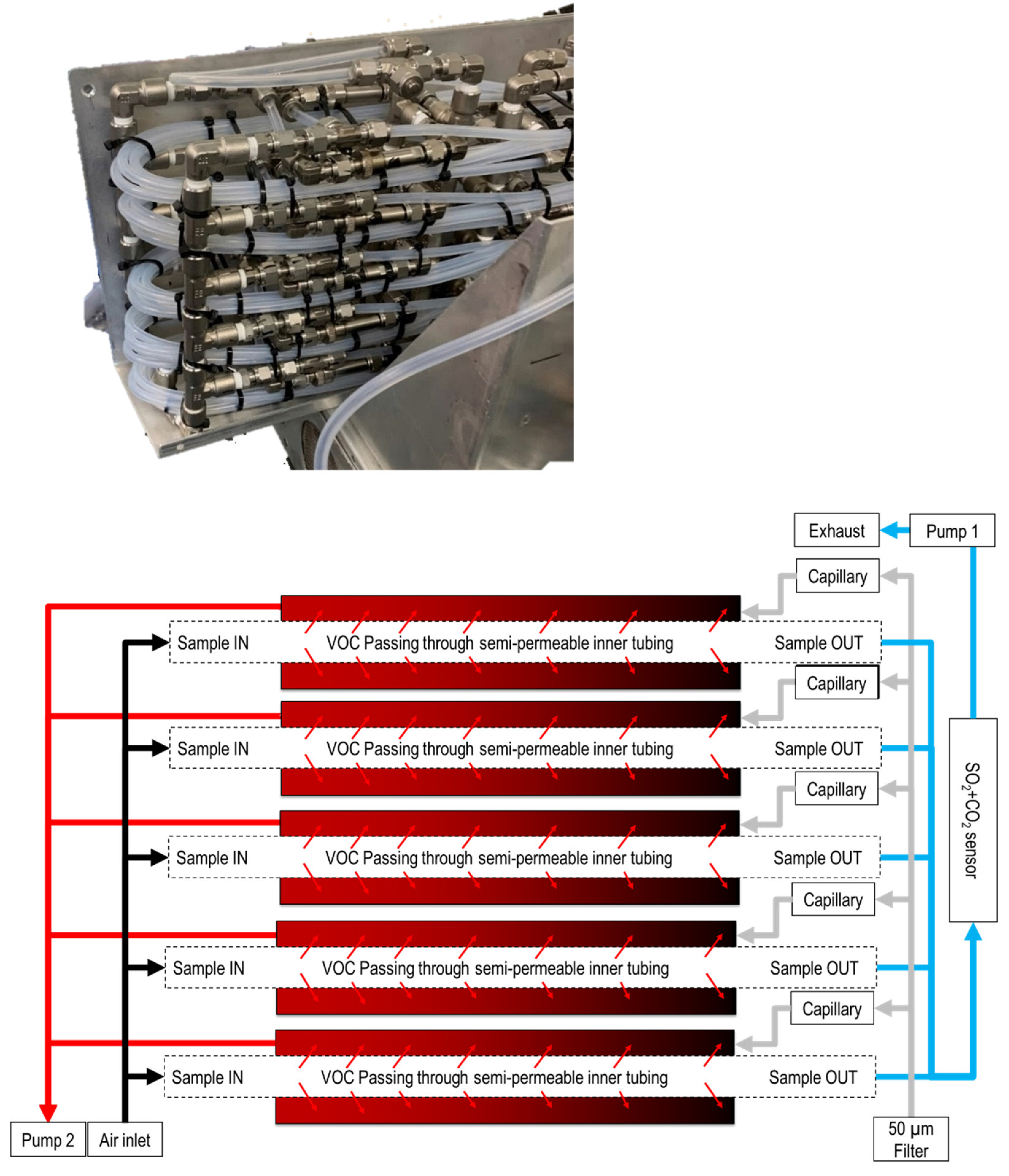
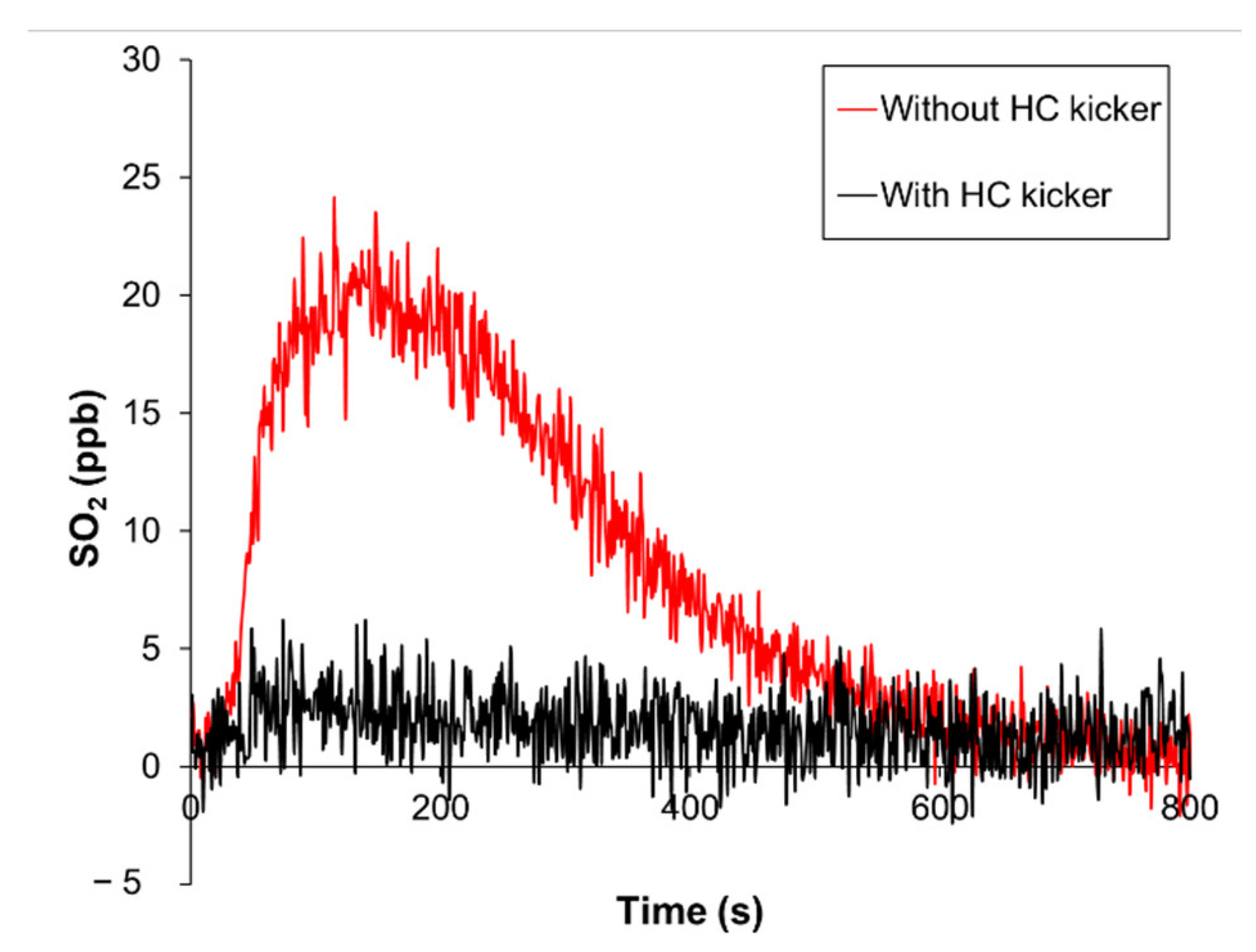
2.3. Hydrocarbon Kicker

Off the shelf, the Thermo 43i TLE instrument is equipped with a hydrocarbon (HC) kicker to remove VOCs from the airflow. This HC kicker consists of (i) an inner compartment, i.e., a very narrow (1/8”) semipermeable tube that is guided inside (ii); an outer compartment, which consists of a standard Teflon tube of 1/4”. The airflow outlet of the outer compartment is connected to (iii); a very thin capillary. The airflow inside the inner compartment is opposite of the airflow in the outer compartment. The inner compartment is connected to the airflow inlet of the SO2 sensor measurement chamber. The outlet of the sensor measurement chamber is connected to the outer compartment. When leaving the other side of the outer compartment, the airflow first goes through a capillary and afterward the vacuum pump. The vacuum pump and capillary create a negative pressure in the outer compartment, thus forcing the VOCs through the semipermeable wall before entering the measurement chamber. The VOCs are disposed of through the air outlet.
However, the standard HC kicker is designed for an airflow of 0.5–1 L/min. The small size of its inner compartment does not allow for a higher airflow with the same VOC removal capacity. The maximum airflow in the sniffer sensor system of 8 L/min was substantially higher than the maximum airflow for a standard HC kicker. The standard HC kicker therefore could not effectively remove the VOCs from the airflow, because of which the HC kicker was removed from the SO2 sensor in the original sniffer sensor design. To solve the VOC error on the SO2 measurements, a novel custom-designed high-volume HC kicker was developed. This high-volume HC kicker is based on ten parallel connected standard (low-volume) HC kickers (Figure 2, upper). In every single standard HC kicker, the airflow was reduced to 0.8 L/min, which is an optimal flow for standard HC kickers. The inner compartment of the novel high-volume HC kicker has a tested total maximum flow of up to 11 L/min at 0.5 bar. However, the maximum flow in the outer compartment at 0.5 bar was limited to 4.5 L/min. Moreover, the original vacuum air pump was not powerful enough to provide the required airflow through the capillaries in combination with the passing of the airflow through the sensors and particle filters. As a result, the standard air pathway through the SO2 sensor was modified and an additional vacuum pump was installed. The original flow in the sniffer sensor was 6 L/min, but by upgrading the existing one-headed vacuum air pump to a two-headed vacuum air pump the airflow was improved to 8 L/min. The pathway was split into two different pathways. The new two-headed vacuum pump was installed behind the SO2 and CO2 sensors, replacing the original one-headed pump. It provided sufficient power to create an airflow through the inner compartment of the HC kickers to meet the increased flow of 8 L/min. However, the pump was not powerful enough to provide the same airflow in the outer compartment due to the capillaries. Accordingly, the original one-headed pump was kept in the system in the form of a second air pathway, providing airflow in the outer compartment and evacuating the VOCs (Figure 2, lower) at 4.5 L/min. This novel design HC kicker with separated airflow had not been applied before and it was unsure if the newly designed high-volume HC kicker would be efficient in removing VOCs at a sufficient rate. Furthermore, it was unsure if the splitting of the air pathways would not result in an unstable pressure or removal of CO2 or SO2.

2.4. Updated Sniffer Sensor Software and Sulfur Emissions Measurements

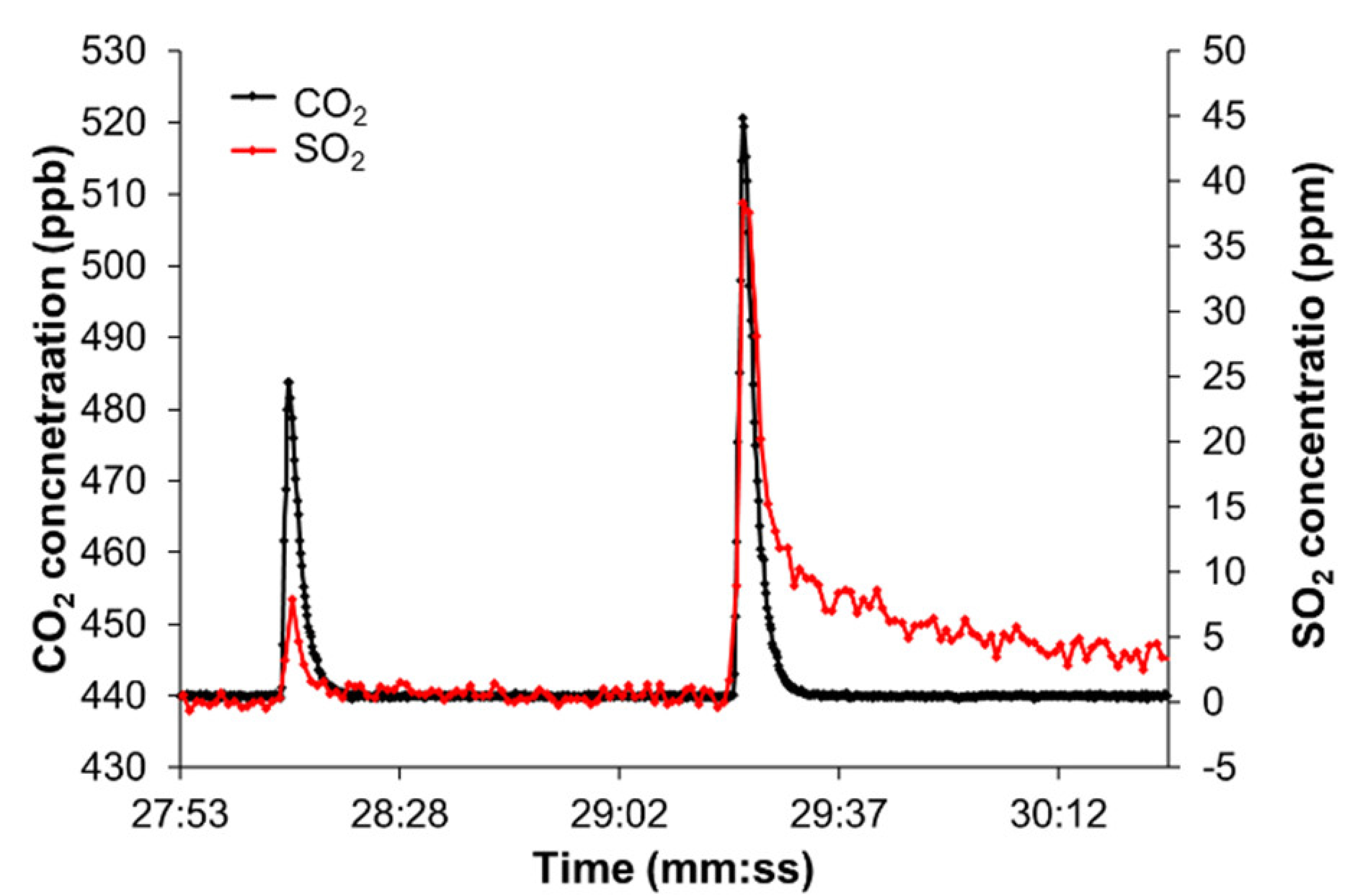
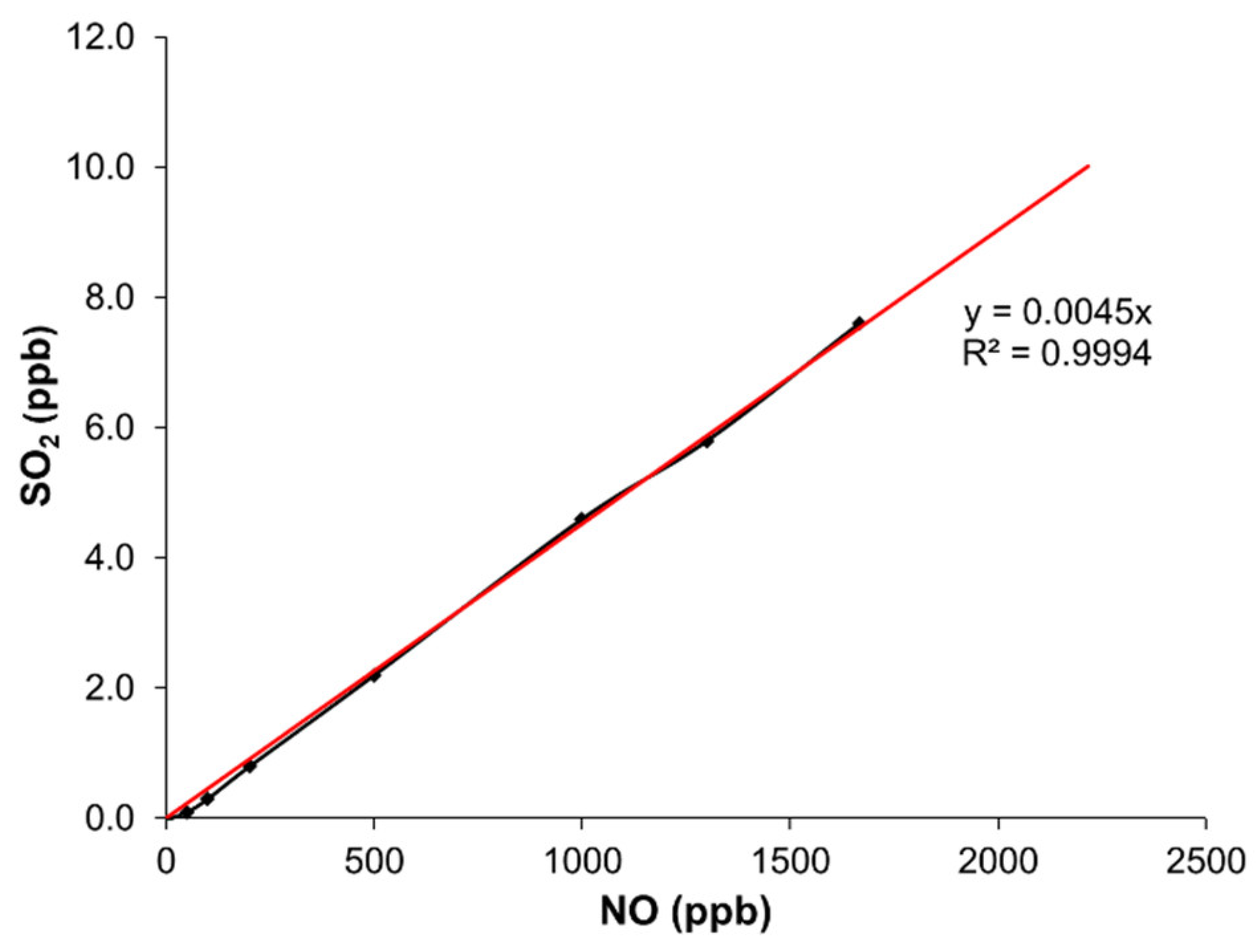
2.4.1. NO Cross Sensitivity

Initially, only the SO2 and CO2 concentrations were used for the calculation of the Fuel Sulfur Content (FSC) [31]. For the determination of fuel quantity, the amount of Carbon (C) was first derived from the CO2 concentration and was subsequently multiplied with a fuel carbon content of 87% [25,32].
F S C = 0.232 ×   [ S O 2 S O 2 , b k g ] p p b d t   [ C O 2 C O 2 , b k g ] p p m d t [ %   S u l p h u r ]
To correct for the NO cross-sensitivity of the SO2 sensor, this formula was adapted by subtracting the measured SO2 from the NO amount in the plume multiplied by the cross-sensitivity factor (CSNO).
F S C N O = 0.232 ×   [ S O 2 S O 2 , b k g ] p p b C S N O × [ N O N O b k g ] p p b d t   [ C O 2 C O 2 , b k g ] p p m d t [ %   S u l p h u r ]

2.4.2. NO Assessment

During the time frame of this study, the NOx sensor on board the aircraft was mainly used for compliance monitoring of MARPOL Annex VI Regulation 13 which introduced limits on NOx emissions [27]. The standard operational modus of the NOx sensor was therefore set to NOx-mode. To estimate the NO concentration from the measured NOx concentrations a default NO/NOx In Stack Ratio (ISR) of 80% was used [33]. The software was modified in such a way that the ratio could be changed in the configuration settings.
F S C N O = 0.232 ×   [ S O 2 S O 2 , b k g ] p p b C S N O × I S R × [ N O x N O x , b k g ] p p b d t   [ C O 2 C O 2 , b k g ] p p m d t [ %   S u l p h u r ]
However, NO/NOx ratios may vary significantly depending on different factors, such as distance to the stack, UV radiation, ambient ozone concentration,… [27,34] Thus, the NO/NOx ratio remained a source of uncertainty. To address this uncertainty, the measurement method was to measure by default in NOx mode. In case the initial NO corrected FSC measurement, based on the NOx concentration and the default NO/NOx ratio (80%) exceeded the operational threshold (Tops) (See Section 3.7.1), the sensor was set to NO mode and two new measurements were made with the NOx sensor in NO mode. Hence, the NO cross sensitivity could be assessed more accurately.

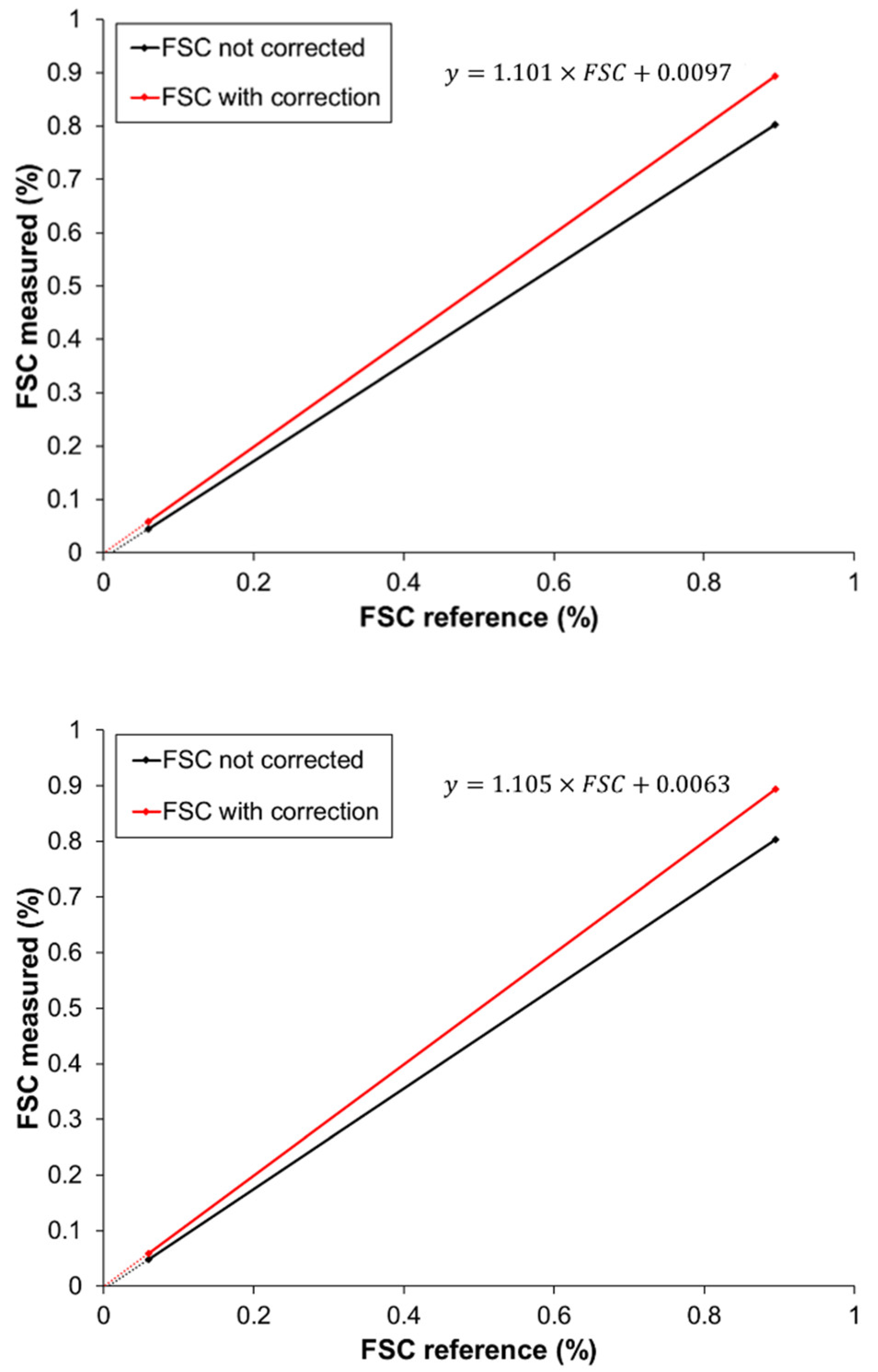
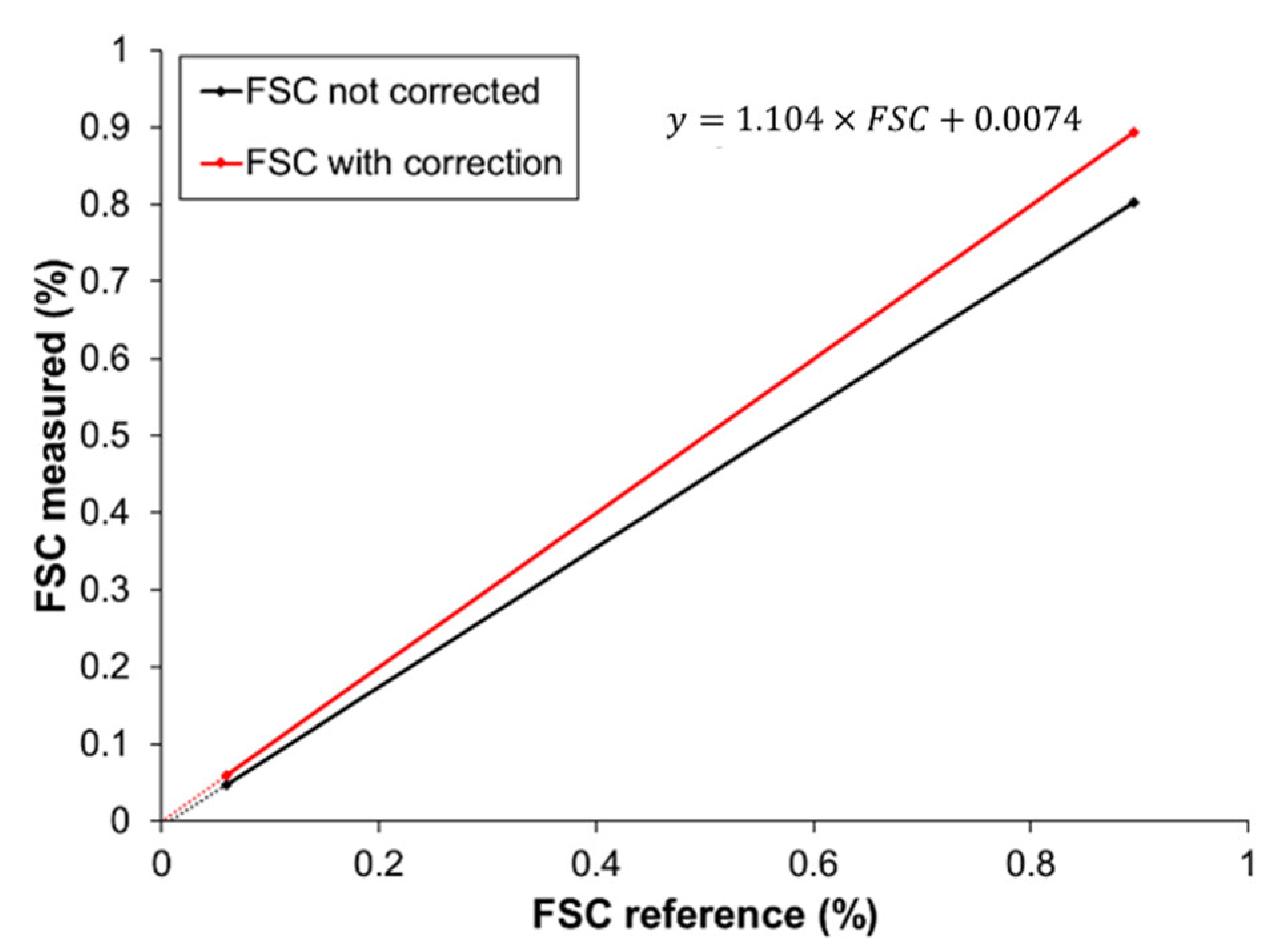
2.4.3. FSC Correction

The FSC measurement was discovered to have a negative bias that consisted of an absolute component (offset) and a relative component (slope) [5]. To be able to calculate the correction factors, two reference points were used to compare the sensor result with the actual value.
For the first set of comparison points (lower FSC values), the median value of all airborne measurements was compared to the median FSC value of 30 randomly selected OGVs that entered Belgian ports. The fuel analysis measurement was executed by the Belgian port inspection authorities using a handheld X-Ray Fluorescence (XRF) scanner (model: Titan S, manufacturer: Bruker).
For the second set of comparison points (higher FSC values), a special gas mixture was ordered from Air Liquide that was utilized to imitate a 1% FSC plume. The ordered concentration was 5000 ppb SO2 with 1000 ppm CO2 in synthetic air. Standard air analyzers are not able to check these high concentrations. As only the ratio of SO2/CO2 was relevant, a PTFE air sample bag of 50 L (manufacturer: Saint Gobain) was used to dilute the mixture with synthetic air (Figure S.1). Afterward, both concentrations of CO2 and SO2 could be measured in the measurement range of the gas analyzers at Brussels Institute for Environmental Management (BIM), which demonstrated that the resulting simulated FSC was on average 0.89% FSC (+/− 0.02%), the difference with the ordered concentration is assumed to be a result of the low accuracy of the plume mixture provided by Air Liquide as the error is in the same order of magnitude of the errors of the reference gasses for SO2 and CO2. This plume simulation mixture was released for a short interval at a high-volume flow in front of the sampling probe to simulate a passage through an OGV exhaust plume, therefore giving the second set of comparison points.
Based on the two sets of comparison points the correction factors could be calculated (see Section 3.5). To be able to calculate the corrected FSC in flight, the IGPS software was modified in such a way that the correction factors were applied during the calculation step and the corrected FSC was immediately provided to the operator after the measurement of the exhaust plume.

2.5. Sniffer Quality Management System

The Sniffer Quality Management System (SQMS) comprises all standard operational procedures (SOPs) that have been specifically developed for the Belgian Sniffer program to ensure measurement reproducibility and guarantee consistent measurement quality and uncertainty. The SQMS is considered a living document that is upgraded on a regular basis. To include the updated measurement techniques the SQMS has been completely revised. The SQMS contains three sections: (i) an operational procedure (OPS) manual; (ii) a quality assurance (QA) manual; and (iii) a data management manual. The revised SQMS can be found in the Supplementary Materials and can be used by other agencies as a guideline to set up their emission measurement program.
The operational procedures have been adapted to include the procedure to remove the NO cross-sensitivity by switching the NOx sensor to NO mode when an initial FSC measurement was observed that exceeded the threshold. In addition, the calibration procedures were adapted to include what was called a quick final check, with the special plume simulation gas mixture of 1% FSC. The SQMS describes that in case the quick final check shows an FSC value deviating more than 10% from the preset value, the calibration procedure is to be repeated, and/or the FSC correction factors are to be adjusted. During the period from 2020–2021, this was never needed during the operations as the factors were regularly monitored and adjusted if needed outside the operations. The adjustments in the QA manual include the maintenance and service of the added hard and software. In addition, the calibration procedure has been described for the special plume simulation gas. The updates to the data management manual include the updated uncertainty calculations and the procedures to measure the actual FSC corrections and how to apply them in the IGPS software. (version 63.99.25.1569)

2.6. Statistical Analysis

The TIBCO Statistica software (version 14.0.0.5) was applied for all statistical analyses in this study. To assess the normality of the SO2 emission measurement data, a Kolmogorov–Smirnov test for normality was used. This test indicated that the data were not normally distributed (p < 0.05). Consequently, the use of parametric tests was not recommended, and nonparametric tests were used. For the comparison of the average emission levels between different monitoring years and ship types, two-tailed Kolmogorov–Smirnov tests were used. Distributions were considered significantly different with p-values < 0.05 [35]. A two-tailed Chi-Square test was used to evaluate frequencies (i.e., compliance rates) between the two groups. Frequencies were considered to be significantly different with p-values < 0.05 [36,37]. When Type I errors are mentioned, they refer to the number of false positives, when Type II errors are used, they refer to the number of false negatives.

3. Results and Discussion

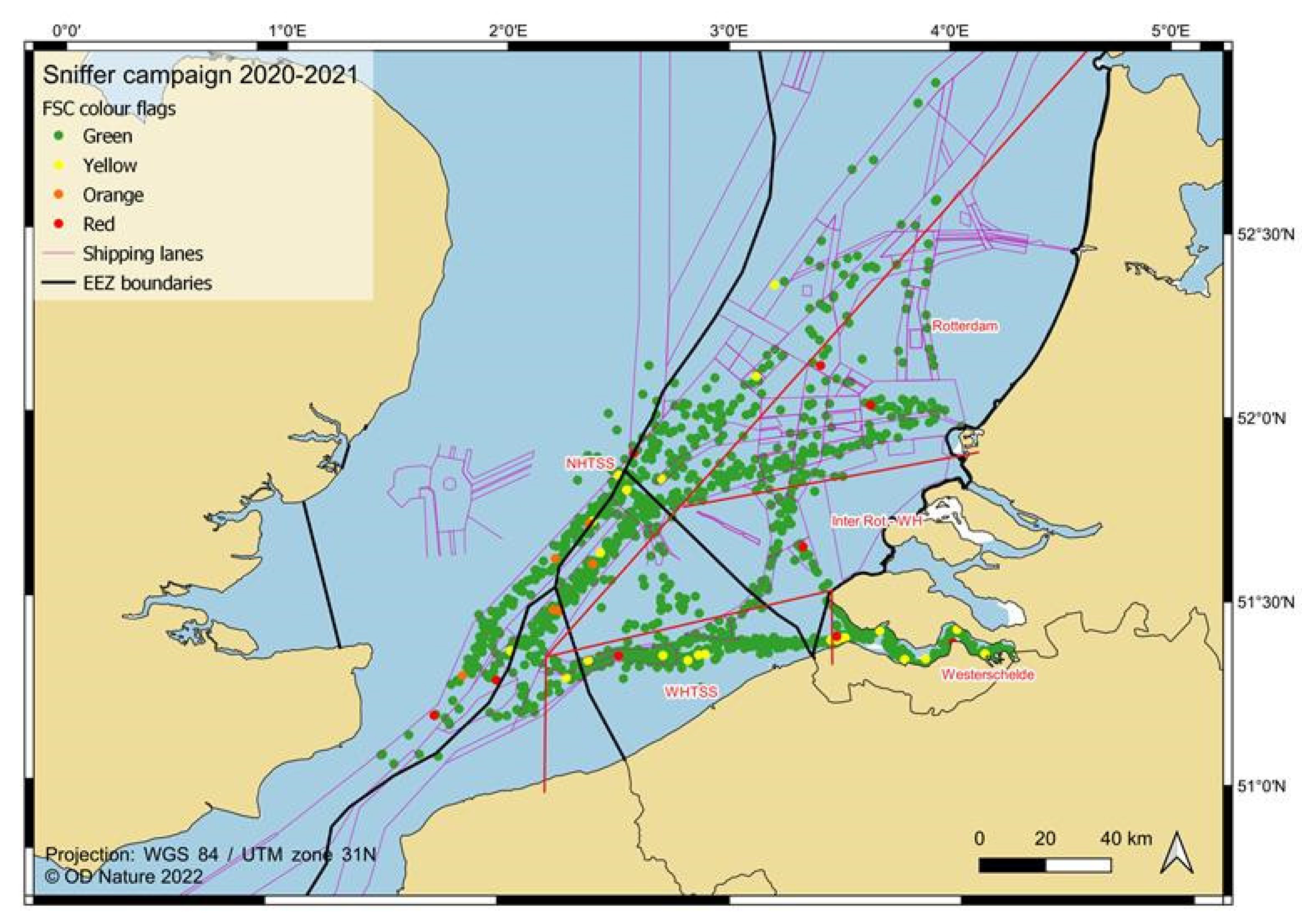
3.1. Monitoring Results

In total, 126 operational flight hours were performed over 83 flights from July 2020 to November 2021. Over 1984 OGV exhaust plume measurement attempts, 1621 successful FSC measurements were made, concerning 1479 OGVs. For 1420 OGVs, the measurements met the quality standards; the others were discarded from the dataset. For 13 OGVs, no NOx was measured due to sensor issues. For the other 1407 OGVs, NOx was measured together with SO2 and CO2.
For 47 OGVs, both NO and NOx emissions were measured, this was conducted for the acquisition of test data (15) and in case an initial potential FSC violation was observed (35) with the sensor in NOx mode. In these cases, after completing an initial measurement with the NOx sensor in NOx mode, the NOx sensor was set to the NO mode for one or two more measurements.

3.2. NO Interference

To assess the NO interference of the SO2 sensor, the sensor was taken to the air quality lab of the BIM, a gas mixture device (MCZ CGM 2000) was used to create airflow with seven different NO concentrations ranging from 0 to 1666 ppb NO (mixed with synthetic air), which indicated that the SO2 sensor had a NO cross-sensitivity of 0.45% and followed a linear pattern with a very high correlation (R2 = 0.9994). The gas mixing device was only able to create gas mixtures of up to 1666 ppb NO at a flow of 8 L/min, falling perfectly in the range of the mean NO concentration of all analyzed OGV plumes (480 ppb). However, the highest observed NO concentrations were higher than the tested maximum concentration (ca. 2200 ppb). Due to the linearity of the measurement principle of the SO2 sensor, this NO cross-sensitivity ratio could be extrapolated to the high end of the measurement range of NO concentrations that were observed with the NOx sensor (Figure 3).

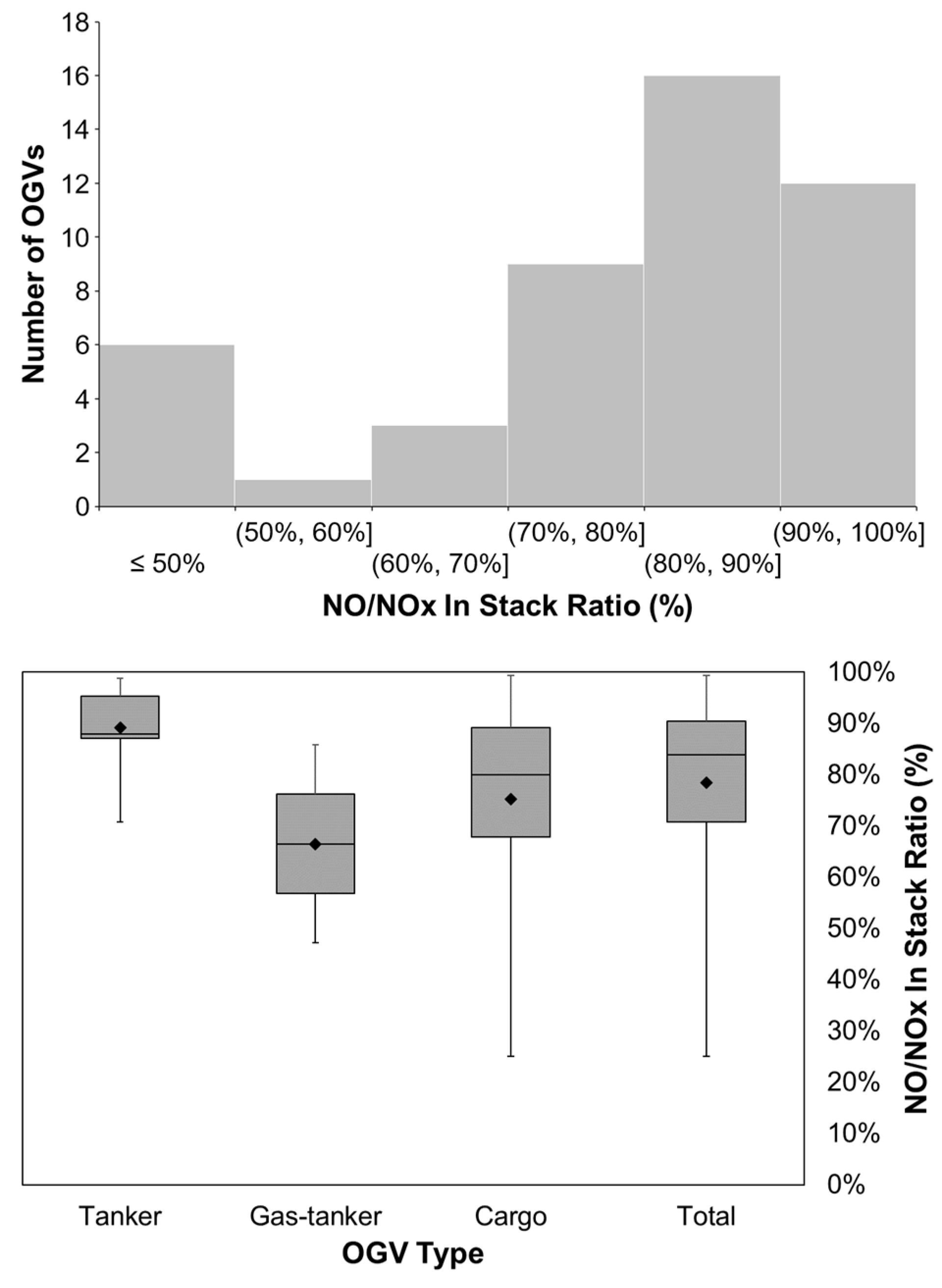
3.3. NO/NOx in Stack Ratio (ISR)

The NO/NOx ISR could not be measured directly as the NOx sensor could only be used to measure either NO or NOx with a time resolution of 1 s. An indirect approach was used to calculate the ISR based on multiple measurements, which measured either the NO or the NOx. As the absolute measurement of NOx and NO is useful due to the high dilution, the NO/NOx ISR ratio was derived indirectly. With this regard, the NO/CO2 ratio was compared to the NOx/CO2 ratio, providing a reliable estimation of the actual NO/NOx ratio.
N O N O x I S R = N O C O 2 N O x C O 2   [ % ]
This illustrated that the NO/NOx ISR ratio had a large variation, going from 25% to 96% (Figure 4, upper). The average value was 78% and the median value was 84%. As the median value is very close to the default of 80%, the latter was not adjusted. However, the large variety of these measurements is in line with the previous findings [34], confirming the importance of using the actual NO concentration to rectify the cross-sensitivity for possible violations, instead of solemnly relying on the default ISR of 80%. By looking at the ISR ratios per OGV type, it was observed that tanker OGVs have generally a higher ISR compared to cargo OGVs (Figure 4, lower). As the actual NO is used for possible violations, the risk of Type I errors is removed. The risk of Type II errors however might be considered for OGVs with a low ISR. In terms of these vessels, a NO cross-sensitivity correction that is too high may be applied resulting in low FSC values. This impact is nevertheless limited for OGVs that are compliant with the NOx emission limits (MARPOL Annex VI Reg. 13) with a relative uncertainty of ca. 10% for Type II errors. The risk of Type II errors increases when there is also non-compliance for NOx observed. To avoid Type II errors in these situations, it is recommended to perform an FSC measurement with the NOx sensor in NO mode, whenever an FSC value is observed close to the threshold, in combination with a possible NOx non-compliance.

3.4. Hydrocarbon Kicker

The effectiveness of the custom-built HC kicker was tested in the lab using solvent-based paint, which is known to contain large amounts of VOCs [38], sprayed on a clod. First, the sniffer sensor was tested without the HC kicker. When the sensor air inlet tubing was held above the paint-sprayed cloth, SO2 values increased to high levels (>20 ppb). Furthermore, a clear SO2 tale was observed that lasted for ca. ten minutes. Then the HC kicker was connected before the sensor air inlet and the procedure was repeated. In this configuration, the SO2 values still produced an increased concentration, but the level was drastically lower (<3 ppb) and within the order of magnitude of the noise of the sensor signal. Moreover, it cannot be excluded that the SO2 peak is not resulting from SO2 released from the paint itself. Within less than three minutes, the smaller SO2 tail was also much shorter than the one without the HC kicker (Figure 5). In addition, the average measured SO2 value was significantly different from the measurements without the HC kicker (p = 0.0). However, it was observed that even with the HC kicker installed, the average value during the VOC exposure (2.2 ppb) was—albeit very limited—significantly higher than the average value before and after its exposure (1.5 ppb) (p < 0.001).
The HC kicker thus showed to be very effective in reducing the VOCs from the airflow in a lab environment. Likewise, the HC kicker, in the field, performed as anticipated. From the moment the HC kicker was put into use, no more tails were observed on the SO2 signal. It can therefore be concluded that, even if the effects of VOCs were perhaps not completely eliminated, the VOCs were more than sufficiently removed and could no longer produce any possible significant effect on the FSC measurements.

3.5. Improvement of Measurement Quality and Reduced Uncertainty

In the previous sniffer campaigns, emission measurements were considered to meet the high-quality standards if the following requirements were met: (i) a distinct link of the plume to a single OGV; (ii) comparable T90 response times for the Thermo 43i TLE and the Licor-7200RS; (iii) ample plume sampling time; (iv) a high to very high Signal to Noise Ratio (SNR); and (v) absence of interference from land-based emission sources [5]. With the increased airflow of 8 L/min instead of 6 L/min, owing to the upgrade of the vacuum pump, the response time and SNR were improved allowing a higher quality of the sniffer measurements. The other quality requirements were not impacted. By improving the airflow, not only the quality was improved, but also the uncertainty was reduced. In addition, by applying a NO correction and removing the impact of VOCs the uncertainty was further reduced.

3.5.1. Improvement of Response Time

Similar to the initial determination of the response time with the previous sniffer version, response times were redetermined by using calibration gases. This allowed the simulation of a concentration–difference (∆C) that is comparable to the measurement of OGV plume exhausts. The T90 response time was defined as the time difference (∆T) between T10, which is the time where the gas concentration is 10% of ∆C above the initial concentration (Cb), and T90, being the time where the gas concentration is 10% of ∆C below the end concentration (Ce)) [5,27].
T = T 90 T 10  
where
C = C 2 C 1
C 1 = C b + 0.1 × C
C 2 = C e 0.1 × C
Both linear and non-linear interpolations were used to find the exact T10 and T90 times [5]. In terms of the Thermo 43i, TLE the non-linear interpolation was considered to be the most appropriate due to the lower signal frequency (1 Hz), which demonstrated that the T90 time was reduced from 3.7 to 3.4 s, an improvement of 9.2% (Figure S3, upper), and well within the average plume sampling time of 8 s (and median of 7 s) [5]. For the Licor-7200RS, no substantial difference was observed between the linear interpolation and non-linear interpolation due to the high-signal frequency (5 Hz). The T90 was reduced from 3.5 s to 3.3 s, also offering an improvement of 9.2% (Figure S3, lower). The T90 times of both sensors were therefore still very comparable with an equivalent improvement of 9.2% as a result of the improved flow of 8 L/min instead of 6 L/min [5].

3.5.2. Improved Signal-to-Noise Ratio (SNR)

The SNR was defined as the ratio of the amplitude of the concentration during plume exhaust measurements (Aplm) over the amplitude of the noise (Abkg) [5].
S N R = A p l m A b k g
A minimum SNR of 20 was previously required for high-quality measurements [5]. In practice, this corresponded to a minimum peak amplitude of 5 ppm, a threshold that was not adjusted. However, the average amplitude of the CO2 measurements increased from 37.3 ppm to 38.5 ppm. As a result, the average SNR of the CO2 measurements was improved from 149 to 154, corresponding to an improvement of 3.4%. The assessment of the average SNR of the SO2 signal is not relevant as this is highly dependent on the average FSC level. The minimum Aplm for SO2 for potential non-compliant OGVs was set at 3 ppb resulting in an SNR of 6.7 which is considered as low, but if a potential non-compliant OGV is observed, in most cases a second measurement will be made. For high-quality non-compliant measurements, a minimum Aplm of 7 ppb SO2 is required. For the large majority of the potential non-compliant vessels, this minimum Aplm was easily reached during one of the measurements with an average Aplm of 51.74 ppb.

3.5.3. Reduced Uncertainty

The combined uncertainty of the FSC measurements (U) was described as the sum of the measurement bias (b) and the standard deviation (utot) [5,39].
U = | b | + σ . u t o t
The measurement bias as described above was defined as an offset in the FSC correction. The average bias for the period from 2020–2021 was 0.0039% FSC, and is 4.6 times smaller than the previous bias of 0.018 +/− 0.005% FSC [5], although it was assumed that the actual negative bias was even lower as the absence of the NO cross sensitivity correction largely eliminated the bias.
The standard deviation was, as for the previous sniffer campaigns, calculated based on the intra-assay coefficient of variability and the sum of all supplementary uncertainty factors (usup,i) [5,39]. The intra-assay coefficient of variability is a measure of the variance of replicate values. The supplementary uncertainty factors include all additional uncertainties for the sensors and methods used for the calculation of the emission factors and are available in Table S1. By using calibration gasses with a lower uncertainty level and with a higher calibration frequency for the reference gasses, the supplementary uncertainty was reduced from 6.15% to 4.36%.
u t o t = ( C V R W ) 2 +   ( u s u p , i ) 2
C V R W = 1 2 i = 1 n ( x i 1 x i 2 0.5 ( x i 1 + x i 2 ) 2 n × 100 ( % )
The CVRW was calculated for three newly defined subsets of FSC values: low FSC values (0.13–0.2% FSC), medium FSC levels (0.2–0.3% FSC) and high FSC values (>3% FSC). The new CVRW values for the different FSC levels are given in Table 1. Due to low degrees of freedom, the normal distribution could not be used and the t-distribution was used instead to replace the σ values.
Based on the updated bias and updated total uncertainties, the combined uncertainties were calculated for the three new FSC levels. When comparing the new combined uncertainties with the previous uncertainty calculation, the updated values may appear to be higher [5]. However, it must be clarified that this is a misconception, as the bias in the previous calculation was underestimated. The bias was most likely much higher but was on average largely removed by the cross-sensitivity to NO. A VOC cross-sensitivity assessment was also not included in the previous uncertainty calculation. Due to the fact that it was not possible to assess the exact bias without the NO cross-sensitivity effect, the negative bias was not applied on an individual measurement level.

3.6. Measurement Results

3.6.1. FSC Correction
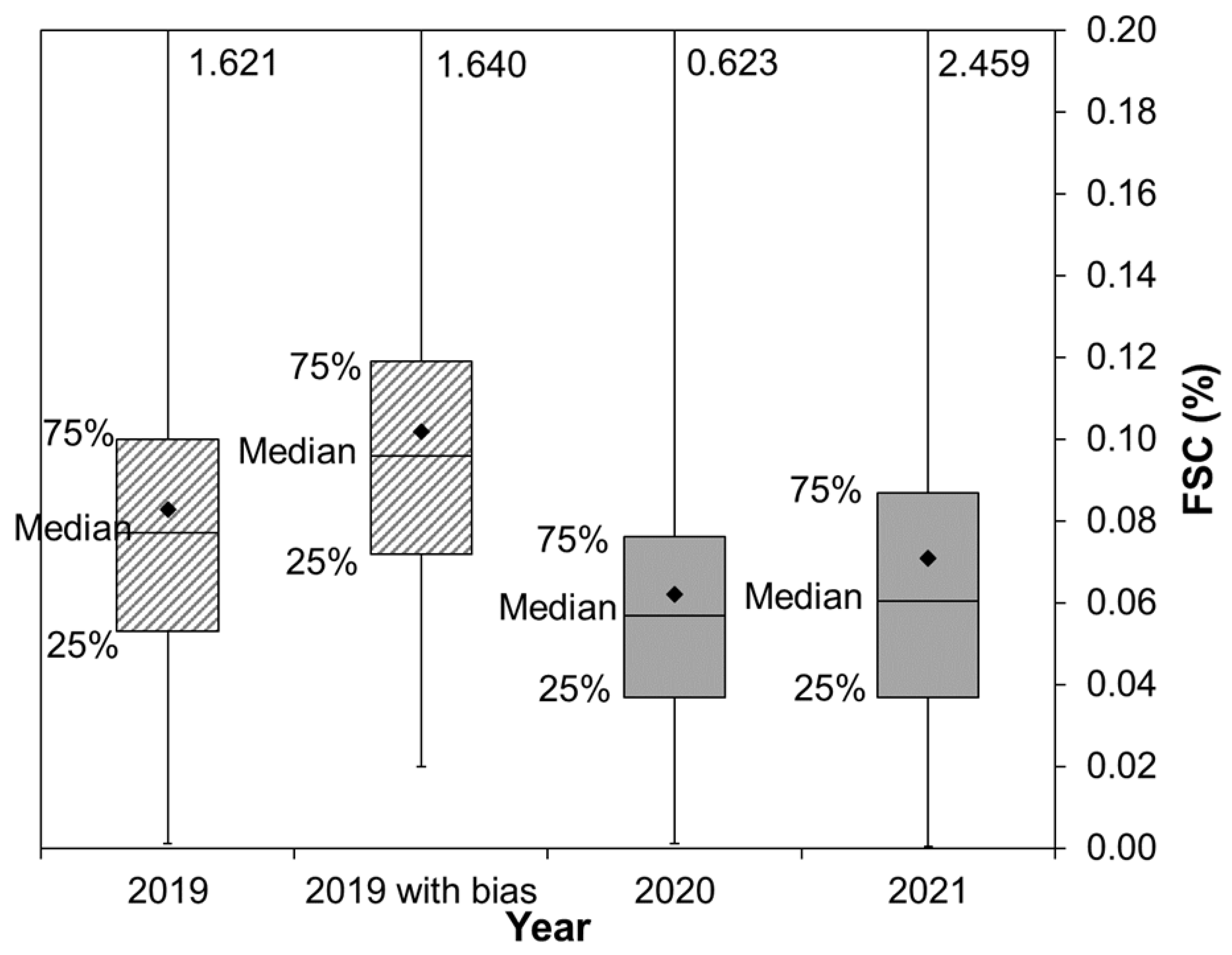
In terms of the offset and slope correction, two sets of comparison points were used, similar to the calibration factors for air analyzers. For the first set of comparison points, the median value of the airborne measurements was compared to the median value of the 30 random fuel analyses in port using a handheld XRF scanner. The differences between the two median values were very small with a median value for the airborne measurements of 0.05% FSC and a median value for the XRF measurements of 0.06% FSC. The 25 and 75% percentiles of the airborne measurements were respectively 0.04 % FSC and 0.08% FSC, while the 25 and 75% percentiles of the XRF measurements were respectively 0.05 % FSC and 0.08% FSC.
In terms of the second set of comparison points, the measured FSC of the special calibration gas mixture was compared to the lab analysis. On average, the simulated plume gas mixture gave a value of 0.80% FSC compared to the 0.89% FSC that was measured in the lab using the PTFE sample bag. For 2020, the resulting slope correction was 10.1% and the offset correction was 0.0097% FSC. For 2021, the slope correction was 10.5% and the offset correction corresponded to 0.0063%. When calculated for the overall period, the slope correction was 10.4% and the offset correction was 0.0074% (Figure 6). These factors were calculated after every check using the mixture gas before every mission and can be updated in the software when a significant variation is observed. The average slope and offset were also applied to reprocess all measurements using the raw data.

3.6.2. Average FSC

The average corrected FSC over the 2020–2021 period was 0.07% FSC, with a median of 0.06% FSC. The annual average FSC for 2020, with an FSC of 0.06%, was significantly lower than the annual average FSC for 2021 of 0.07% FSC (p < 0.01) (Figure 7). The median values, however, are not that different, which indicates that the used fuel does not seem to vary between 2020 and 2021. The higher average is most likely a result of higher extreme values in 2021. When comparing the average FSC between the periods of 2020 and 2021 with the period of 2019 (0.08%), a significant decrease in average FSC was observed for both 2020 and 2021 (p < 0.001). This is even without applying a bias correction for the 2019 data. When the bias of 0.0189% FSC [5] was applied, the actual average FSC for 2019 increased to 0.10% FSC.

3.7. OGV Compliance Analysis

Thanks to the improvement of the measurement quality and the reduction of the uncertainty, it was possible to improve the assessment of OGV compliance with MARPOL Annex VI Regulation 14. For the assessment of compliance during the surveillance operations, a set of three operational reporting thresholds (TOPS) with corresponding color flags were created in 2016 [5]. These TOPS were updated with reduced uncertainty levels.

3.7.1. Lowered Compliance Thresholds

The TOPS used for different non-compliance alert levels are based on the combined measurement uncertainty (U) and sulfur limit (S). In comparison with the previous method, the bias was integrated into the FSC calculation and could therefore be removed from the equation for the threshold calculation [5].
S   ( % F S C ) = T a ( 1 σ × u t o t )
The actual threshold (Ta) was described as the FSC value for which the difference between its value and its combined uncertainty exceeded a pre-defined S which depends on the color flags [5,27]. The value for S is based on the legal follow-up applied in Belgium. A warning is given from 0.11% FSC, and an administrative penalty is applied from 0.15% FSC [5]. As the degrees of freedom of the datasets per FSC level were not sufficient to allow the use of a normal distribution, t values were used instead of σ values
T a = S 1 t × u t o
The same three color flags were used for creating the new thresholds. However, the thresholds were reassessed due to the updated uncertainties. The yellow flag represented the lowest alert level with a confidence interval (CI) of 60% (t = 0.86). Its operational reporting threshold was lowered from 0.15% to 0.13% FSC. As in the FSC calculation before 2019, the positive bias was not included in the actual threshold and was 0.17% FSC, hence the improvement of the threshold was 0.04% FSC or an improvement of 23%. The orange flag indicated a medium alert level, with a CI of 95% (t = 2.179). Its threshold remained at 0.2% FSC, but as the bias was not included in the previous orange flag, the actual improvement was 0.02% FSC or 10%. Red flags represented high non-compliance alerts with a CI of 99% (t = 2.528); the red flag threshold could be reduced from 0.4% to 0.3% FSC. Likewise, the bias was not taken into account with the threshold. In case the bias was to be included, the previous threshold would in fact be 0.42%, and the actual improvement would therefore be 0.12% FSC, which represents an improvement of 30%. The thresholds for the orange and red flags are in fact even lower, but were rounded up to create operational thresholds (TOPS) that are easy to memorize and apply in surveillance and enforcement operations, whilst remaining on the safe side for avoiding Type I errors (Table 2).
When a sulfur limit of 0.11% FSC would be applied for the red flag instead of 0.15% FSC, with the updated uncertainty, the CI increases even to 99.99% for the same threshold (0.295% FSC).
In the aforementioned uncertainty calculation, the uncertainty was calculated for individual measurements. When conducting multiple measurements, the uncertainty of the average value can be divided by the square root of the number of measurements (n).
u n = u t o t n  
For possible non-compliant OGVs, a confirmation measurement was made in almost all cases, which means that in the case of alerts, the actual uncertainty was even lower and uncertainty thresholds could potentially be further reduced (Table 3).
By taking two measurements it is possible to state that observed non-compliant values of more than 0.198% FSC (orange flags) are above the sulfur limit of 0.11% with a CI of 99.99%.

3.7.2. Evaluation of Non-Compliance

An OGV was considered to be non-compliant when it was measured with a value exceeding the yellow threshold. As non-compliance can, strictly speaking in accordance with the EU Sulfur Directive (2016/802) [3] and the European Commission Decision (2015/253) [7], only be legally proven with a positive fuel sample taken in port. All non-compliance detections at sea referred to in this evaluation are expressed as alleged non-compliance. In nearly all instances when a measured OGV was found to be potentially non-compliant, a second and third measurement was performed to confirm the initial measurement, with the NOx sensor in “NO mode”. As the initial measurement was performed with the NOx sensor in “NOx mode”, and was therefore characterized by a higher uncertainty due to the uncertainty in the NO/NOx ratio, it was chosen to not rely on this first measurement but only use the measurements made with the NOx sensor in “NO mode” for the assessment of alleged non-compliance. This implied that, after the NOx sensor was switched to the “NO mode”, two additional measurements were required. If the second measurement (first in “NO mode”) did not confirm the initial value, the OGV was reported as compliant to avoid Type I errors. In case the second and third measurements confirmed the first measurement, only the latter values were reported. If the two latter measurements were assigned to different alerting color flags, the lower alert level of the two was used as a precautionary measure to avoid overestimating the FSC value.
For 2020 and 2021, the FSC measurements were recalculated using the overall offset (0.0074% FSC) and slope correction (10.4%). These FSC values were compared to the updated compliance thresholds and resulted in 35 alleged non-compliant OGVs. In the same period, only 22 OGVs had been reported to port inspection authorities. For 13 OGVs, the initial measured FSC value was below the threshold, but by applying the span and offset, the corrected FSC value slightly exceeded the yellow color flag threshold.

3.7.3. Compliance Rate Comparison

The overall compliance rate was 97.3% for both 2020 and 2021. When looking in more detail at the distribution of the compliance levels between 2020 and 2021, it was observed that the number of red flags was slightly higher for 2021 (0.7%) compared to 2020 (0.5%). Furthermore, the number of yellow flags was higher for 2021 (1.7%) compared to 2020 (1.5%) and the number of orange flags was higher for 2020 (0.7%) compared to 2021 (0.3%). None of these frequencies were significantly different between 2020 and 2021. However, when comparing the compliance over the period 2020–2021 with the compliance for the year 2019 (95.9%), the difference was found to be significant (p = 0.0445). This is remarkable since the thresholds for 2019 were higher. If the same updated thresholds were to be applied to the 2019 data, the compliance level for 2019 would be 93.0%. If in addition, the bias of 0.0189 were to be applied, the compliance in 2019 would even fall to 85%. When looking at the red flags only, the 0.6% red flags in 2020–2021 were lower compared to the 0.9% in 2019, but this difference was not significant (p = 0.5). Consequently, it can be concluded that the compliance rate was substantially improved between 2019 and 2020, but concerns remain about the minor number of gross polluters (red flags).

3.7.4. Global Sulfur Cap and Global Bunker Fuel Prices

An explanation for this drastic improvement in compliance levels can be located in the implementation of the ‘Global Sulfur Cap’ and ‘Carriage Ban’. Before 2020, OGVs were allowed to use Heavy Fuel Oil (HFO) of up to 3.5% FSC outside a SECA. As the fuel cost can contribute up to 50% or more of the operating costs of OGVs [40,41], the fuel prices and especially the price difference between compliant and non-compliant fuel may be an important driving force for non-compliance.
From 1 January 2020, the Global Sulfur Cap entered into force, as a result of which the FSC was limited worldwide to 0.5% [42]. Shortly after, from 1 March of the same year, the carriage of non-compliant fuel oil (i.e., HFO) for combustion purposes for propulsion or operations on board OGVs became prohibited, unless the OGV was equipped with an EGCS [43]. At the start of 2020, the price for Very Low Sulfur Fuel Oil (VLSFO), i.e., fuel oil with an FSC of 0.5%, was 598 $/ton in the port of Rotterdam (price on 6/01/2020). The price for Ultra Low Sulfur Fuel Oil (ULSFO), fuel oil with an FSC of 0.1%, was at that moment slightly lower at 593 $/ton. The price for Low Sulfur Marine Gas Oil (LSMGO) was 623 $/ton and thus very comparable with the price of VLSFO. At that moment, the price difference between SECA-compliant fuel and Global Cap Compliant Fuel was small. Therefore, it was economically speaking not profitable for OGVs to be non-compliant in a SECA. The HFO price was at that moment 304 $/ton much lower
From the start of 2020, prices decreased gradually until March 2020. From that moment onwards, due to the impact of the global Covid-19 pandemic, all fuel prices dropped by about 60%. On 28 April 2020, the fuel prices were reduced to 150 $/ton for VLSFO, 160 $/ton for ULSFO and 180 $/ton for LSMGO. The price difference in this period was still very small and also the price for HFO decreased, but less dramatically to 123 $/ton.
Due to the slow economic recovery following the aftermath of the global Covid-19 pandemic, fuel prices gradually started to increase again. The main turning point was the start of 2021; from that moment the price difference between ULSFO and VLSFO generally increased. By the summer of 2021, prices were again at the same level as at the beginning of 2020. The largest price difference in 2021 was observed on 18 October 2021 at a price of 606 $/ton for VLSFO, 710 $/ton for ULSFO and 724 $/ton for LSMGO, resulting in a price difference of 104 $/ton between VLSFO and ULFSO. For an OGV with fuel consumption of 200 tons/day, the potential economic gain of non-compliance was 20,800$ per day.
Recent dramatic developments in 2022, however, changed the global economic context so profoundly that the demonstrated improvement of OGV compliance levels for 2020 and 2021 would probably be stopped or reversed. Since the Russian invasion of Ukraine on 24 February 2022, the price difference increased to unseen record heights. On 3 May 2022, the price was 647 $/ton for HFO, 822 $/ton for VLSFO, 1270 $/ton for ULSFO and 1338 $/ton for LSMGO. The price difference between VLSFO and ULSFO was at that moment a staggering 517 $/ton (Figure S4). For a large container OGV (+10,000 Twenty-foot Equivalent Unit (TEU)), the average daily fuel consumption is in the range of 124 up to 367 tons/day [41]. This led to a potential economic gain of up to 190,000$ per day. (All prices above are for the port of Rotterdam and were provided by Ship & Bunker).
With this important price difference in 2022, a decrease in the compliance rate in 2022 was expected. Although at the moment of publication, the data for 2022 was still incomplete, the preliminary results for the compliance rate for the period 14 March 2022 until 3 August 2022 have thus far shown a significant decrease in the compliance rate to 95.2% (p = 0.0246). This confirms the negative compliance prognosis. Additionally, the average FSC was with 0.078% higher in this period than the average of 2021, although this difference was not found to be significant (p > 0.1).
The graphs in Figure S4 demonstrate the impact of the absolute fuel price for MGO and the spread between ULSFO and MGO on the monthly average FSC and the non-compliance rate. The correlation between the monthly average FSC and the price for MGO is nevertheless low (R2 = 0.294). The correlation between FSC and the price difference between ULSFO and MGO is slightly higher (R2 = 0.330). A stronger correlation was found between the non-compliance rate and the price for MGO (R2 = 0.816) and a slightly higher correlation was found when comparing the fuel price difference with the non-compliance rate (R2 = 0.818). Furthermore, the slope of the linear regression is higher when the price difference is plotted against both the average FSC and non-compliance rate, compared to when the absolute price of MGO is plotted against the average FSC and non-compliance rate. This indicates that the price difference between high-sulfur fuel oils and low-sulfur fuels plays a more important role in compliance behavior than the absolute fuel price.
Another important explanation for the improved compliance from 2020–2021 is that it follows a downward non-compliance trend that has been initiated long before the implementation of the Global Sulfur Cap. This trend shows that the monitoring and enforcement efforts in Belgium and other European countries are paying off.

3.7.5. Compliance of OGVs with a Scrubber Installation

MARPOL Regulation Annex VI provides the possibility to use scrubbers, to continue using fuel with higher sulfur content, under the condition that emission limits are comparable to the SO2/CO2 emission ratios of OGVs running on compliant fuel [13,14,15]. Table S2 provides the ratios corresponding to the allowed FSC, which are in fact based on the same emission factor calculation as provided in Formula 1.
S O 2 ( p p m ) C O 2   ( %   V V ) = 10 × S O 2 ( p p b ) C O 2 ( p p m ) = 10 × F S C   ( % ) 0.232
OGVs equipped with a scrubber are allowed to use fuel oil with a very high percentage of sulfur (i.e., HFO). It has already been demonstrated that open-loop scrubbers create significant risks for the marine environment due to the release of scrubber wash water, in particular in densely navigated coastal waters [15,16,18]. But paradoxically they may also pose a significant risk of more air pollution in certain cases. Non-compliance may occur intentionally; for instance, the scrubber may be under scrubbing or may be switched off altogether, to lower the fuel consumption and/or energy demand from the scrubber. The pumps of a scrubber system have a very high power demand and may consume up to 10% of the generated electricity capacity [24,44,45]. Non-compliance may also occur due to negligence, when no action is taken after technical failures, or system-generated alarms. Non-compliance may furthermore occur unintentionally when the emission monitoring system on board is malfunctioning. These gas emission sensors are only calibrated occasionally (i.e., once per year). If in between calibrations a sensor is no longer providing the correct gas measurements, the SO2/CO2 ratios are no longer correct and may result in under or over scrubbing. Finally, “allowed” non-compliance can also occur either during the commissioning phase (a short period after the installation of the scrubber on board the OGV) or even for short periods during regular operations. The IMO guidelines allow for a one-hour non-compliance, and if in that short time window the situation cannot be resolved, the coastal state, port state and the OGV flag state must be informed [14]. However, if non-compliance occurs by OGVs equipped with a scrubber, this will almost always result in higher sulfur emissions compared to non-compliant OGVs without a scrubber, since the latter will, in most cases, be using VLSFO of 0.5% FSC.
In the period from 2020 and 2021, 38 possible non-compliant OGVs have been observed, of which 15 of these OGVs were equipped with a scrubber. When focusing on the higher observed FSC levels, six OGVs were observed with an FSC higher than 0.5% and five of these OGVs were using a scrubber system, as was indicated in the Thetis-EU database. The other OGV was most likely also equipped with a scrubber system, but this could not be confirmed. When focusing on all observed red flags, it can be concluded that at least six (but most likely seven) out of the total observed nine red flags from 2020–2021 concerned OGVs with scrubbers (i.e., 67%). In the case of yellow and orange flags, 10 out of 29 OGVs were equipped with a scrubber. This is in line with the global ratio of OGVs equipped with a scrubber, as by the end of 2021 ca. 30% of the global fleet was equipped with a scrubber system [21], which indicates that OGVs with scrubbers have a comparable amount of low to medium non-compliance levels as non-scrubber OGVs, but are twice as much observed with high non-compliance levels. It must be highlighted that the higher amount of non-compliant scrubber OGVs may be a temporary issue due to the limited experience a seafarer may have with the technology. Several shipping companies, such as Stenalines and Bore, operating in the surveillance area with scrubber OGVs have been observed frequently, and although there were some initial non-compliant observations at the start of the scrubber operations (during the commissioning phase), these OGVs now have a very high (up to 100%) level of compliance.

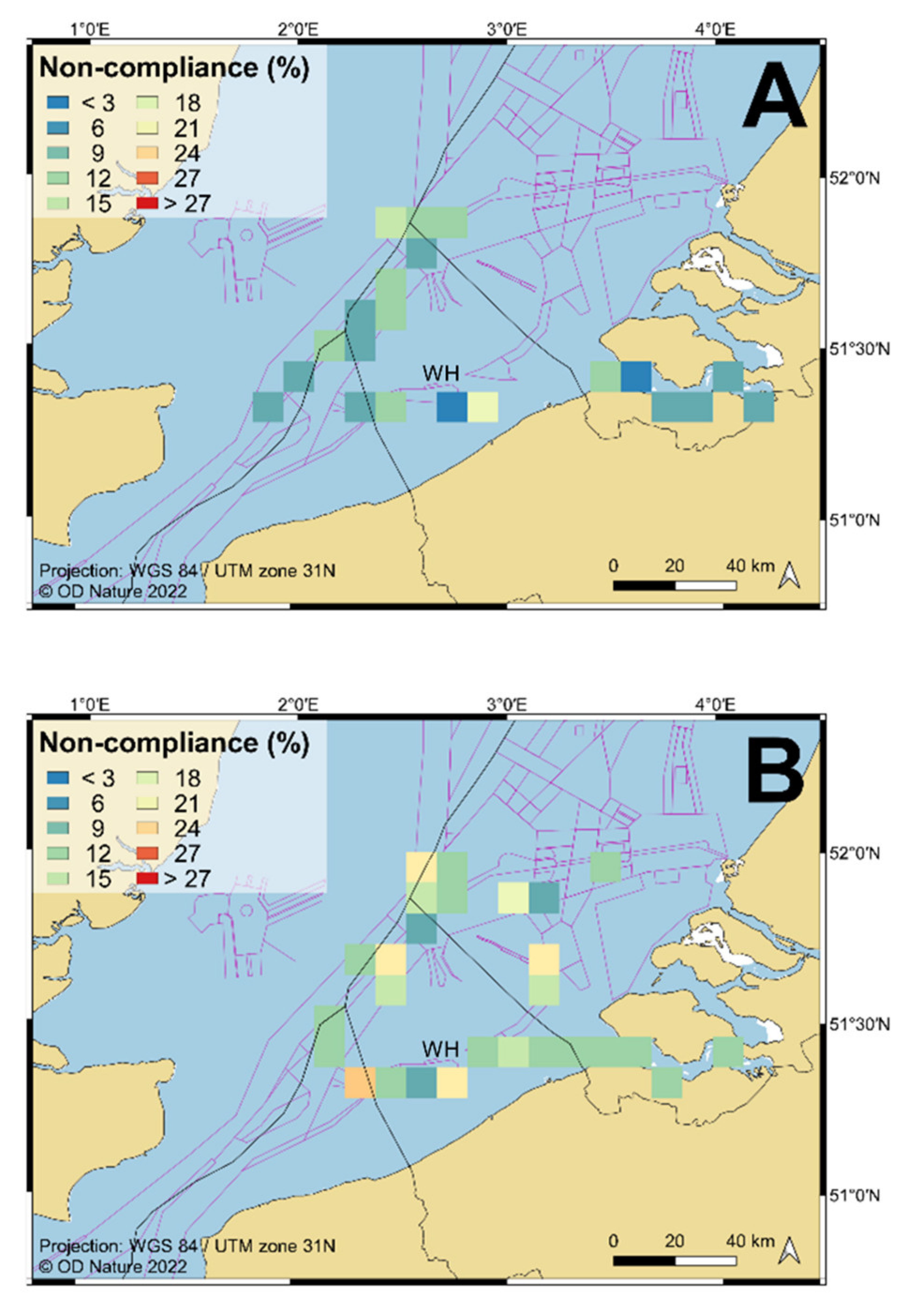
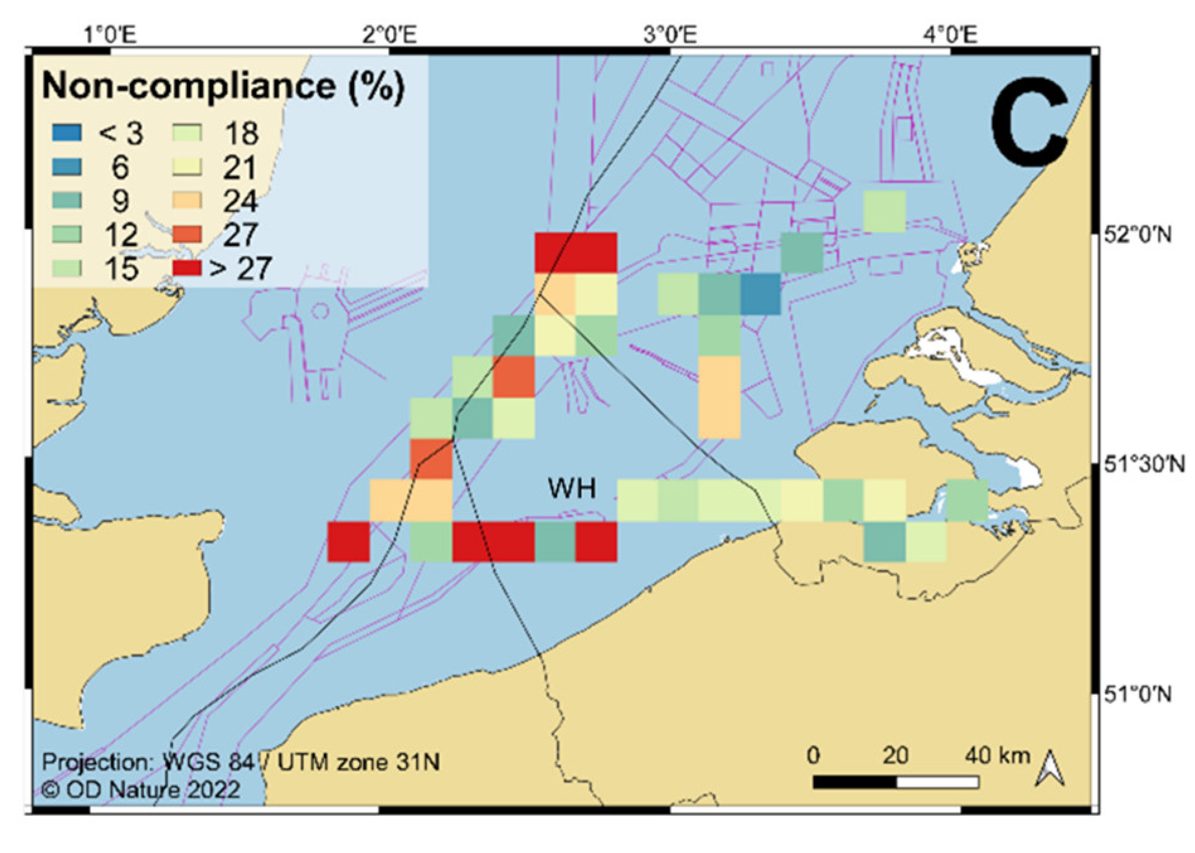
3.7.6. Geospatial Analysis

When comparing non-compliance levels between the different zones (NHTSS, WHTSS, Westerschelde, Rotterdam and the zone between WHTSS and Rotterdam) that were identified in the 2015–2019 study [5] (Figure 8), there were no significant differences observed (p > 0.05); although the non-compliance was slightly higher for the NHTSS, especially when focusing on non-compliance levels from 0.2% FSC. The average FSC level for the Westerschelde was 0.08%, significantly higher than in the other zones (p < 0.05); although this result was biased by a single OGV equipped with a scrubber that was observed with an FSC of 2.35%. However, even when this vessel was excluded from the data, the average is still significantly different (p < 0.05).
When comparing the spatial distribution of non-compliant OGVs in the period from 2020–2021, there were slightly higher non-compliance levels observed in the WHTSS and NHTSS shipping lanes compared to the Westerschelde, with non-compliance levels ranging between 1% and 18% per grid cell of 5 km, with one outlier at the West Hinder Anchorage area (WH) (Figure 9A). This is in line with the spatial analysis of the compliance data from 2015–2019 [5] that was performed with the previous thresholds and methodology. The data from 2019 have been reanalyzed using the lowered thresholds of 2020 (Figure 9B) and resulted in overall higher non-compliance levels, confirming the spatial distribution with higher non-compliance in the main offshore shipping lanes. When the 2019 data is further corrected with the bias of 0.0189% FSC (Figure 9C), the difference in compliance compared to 2020–2021 is striking, with non-compliance levels between 6% and 30% per grid cell. Although caution needs to be applied in the interpretation of the 2019 data for the measurements that fall between the old and new thresholds, the OGVs were at that moment deemed compliant and therefore only one measurement was made. From 2020–2021, two measurements were made and in case one of the two was below the threshold, the lowest of the two was withheld to assess compliance. Furthermore, as was demonstrated in Section 3.2, there is a potential impact of the NO cross-sensitivity. This cross-sensitivity was included in the calculation of the bias. However, this was based on average NO emissions comparable to the Tier I emission levels. It was established that about 4% of the OGVs are not compliant with MARPOL Regulation 13 [27] and, therefore, emit significantly higher levels of NO. For these reasons, the non-compliance levels in Figure 9C are certainly an overestimation, the actual non-compliance levels must therefore lie between Figure 9B,C.

4. Conclusions

Airborne measurements of FSC are not yet used as official and conclusive evidence for prosecution and sanctioning OGVs for violations of MARPOL Annex VI Regulation 14. However, these measurements provide a valuable non-compliancy indication that can be used to target potential violators for further inspections in the port. This paper demonstrates that the previous airborne sniffer methodology for the monitoring of compliance to sulfur regulation by OGVs, based on the SO2/CO2 ratio, has been substantially improved by applying novel features. Thanks to the upgraded vacuum air pump, the updated sniffer sensor system has a shorter response time (−9.2%), a higher SNR (+9.6%) and an increased flow, which drastically improved the quality of the sniffer measurements. Additionally, by including the NOx sensor and measuring the NO concentration after an initial potential non-compliance was observed, the cross-sensitivity to NO was removed. With the introduction of a novel high-volume HC kicker with separated airflow, the impact of VOCs on the SO2 measurements was removed. Finally, a procedure was developed to assess the proportional bias and absolute bias before ever using a special plume simulation mixture. Thanks to these modifications in the sniffer hardware and SOPs, uncertainty was considerably reduced. Owing to this reduced uncertainty, compliance thresholds could be lowered to 0.13% FSC for yellow flags and 0.3% FSC for red flags.
The average observed FSC of 0.07% for the period from 2020–2021 was significantly lower than the average FSC of 0.08% for 2019. If the bias were to be applied to this average FSC, the average FSC for 2019 could even be as much as 0.10%. The application of the improved thresholds resulted in an overall compliance rate of 97.3% with MARPOL Annex VI Regulation 14 for 2020–2021, which is significantly higher in comparison to the compliance rate of 2019 (95.9%). However, we need to take into account that the measurements in 2019 used a different methodology making it difficult to accurately compare compliance levels. In case the data in 2019 were to be assessed according to the 0.13% FSC threshold, compliance levels would be 93%; and in case the data in 2019 were to be corrected with the bias of 0.0189% FSC, compliance levels for 2019 could even be as low as 85%—although the latter is probably an overestimation (for aforementioned operational reasons).
Regardless of a potential comparison bias between the 2019 data and the 2020–2021 data, compliance levels improved drastically from 2020 onwards. This positive development coincided with the implementation of the Global Sulfur Cap in January 2020. Therefore, this regulatory measure can be seen as a crucial driving force for the improvement in compliance behavior and a further reduction of air pollution from OGVs. Nevertheless, the collapse of fuel prices in 2020 due to the global Covid-19 pandemic and the equal price for high- and low-sulfur fuels in this period need to be taken into account as well. Additionally, the monitoring and enforcement activities conducted by different European member states should be considered as a potential driver in the increased compliance rate. It should be noted that although the number of red flags also reduced between 2019 and 2020–2021, this was not regarded to be significant. This means that gross polluters remain a reason for concern in the future.
The annual average FSC of 0.06% for 2020 was significantly lower than the annual average FSC of 0.07% for 2021. The increased FSC values for 2021 and improved compliance in 2020 and 2021 can be explained by the evolution of fuel prices. As a result of the Global Sulfur Cap, OGVs were forced from 2020 onwards to operate on VLSFO. In 2020, the average price spread between VLSFO and LSMGO of 39$ was relatively low, but in 2021 the price difference increased to 65$. The largest price spread that year was observed on 18 October 2021, with a price difference of 104 $/ton between VLSFO and LSMGO. This could explain the higher observed average FSC for 2021. For an OGV with fuel consumption of 200 tons/day, the potential economic gain of non-compliance contributed to 20,800$ per day. Unfortunately, the war in Ukraine pushed the price difference between high and low sulfur fuels to unseen heights with an average price spread of 231$ in 2022 (until 12 May 2022), and an unprecedented maximum price spread of 517 $/ton on 3 May 2022, creating a potential economic gain of more than 100,000$ per day for that same OGV with daily consumption of 200 tons/day. Accordingly, it can be expected that the average FSC and non-compliance for 2022 will increase again (as already indicated by preliminary sniffer flight results for the first part of 2022). The new techniques described in this research provide a solution for effective and more refined offshore compliance monitoring in the future.
Another important benefit of the airborne monitoring method lies in its potential to effectively monitor and target scrubber OGVs. Special attention should be paid to these scrubber OGVs as, in case of non-compliance, they generally have much higher FSC levels (>0.5%) compared to OGVs that are not equipped with a scrubber. Inspections of these systems are laborious, time-consuming and not highly effective. The targeted information resulting from airborne monitoring has the potential to drastically improve scrubber inspection efforts in port. This is not only important for port inspection authorities, as shipping companies that abide by the rules will profit, because compliant OGVs will be less likely to be targeted by an inspection in port. This will save time and money for the shipping company and also contribute to the creation of a level playing field.

Supplementary Materials

The following supporting information can be downloaded at: https://www.mdpi.com/article/10.3390/atmos13111756/s1, Figure S1. Schematic overview of the updated sniffer sensor system, with NOx sensor and HC kicker; Figure S2. PTFE sample bag of 50 l filled with 2.5 l of the plume simulation gas mixture and further filled with synthetic air; Figure S3: T90 response times for the Thermo 43i TLE sensor and T90 response time for Licor 7200 RS. At airflow of 8 l/min; Figure S4. Evolution of the bunker fuel prices for Rotterdam (own visualization based on data provided by Ship and Bunker); Figure S5. Graphs demonstrating the relation between price of MGO in Rotterdam compared to the monthly average observed FSC (A) and the monthly observed non-compliance rate (B). Graphs demonstrating the relation between the price difference or spread between MGO and VLSFO in Rotterdam compared to the monthly observed FSC (C) and the monthly observed non-compliance rate (D); Table S1. Supplementary uncertainty factors and the combined supplementary standard uncertainty; Table S2. Emission ratios for EGCS systems; Table S3. Observed color flags and non-compliance levels for the different zones; Sniffer Quality Management System.

Author Contributions

Conceptualization, W.V.R.; Data curation, W.V.R.; Formal analysis, W.V.R.; Funding acquisition, K.S.; Investigation, W.V.R., A.V.N., K.S. and B.V.R.; Methodology, W.V.R.; Project administration, K.S.; Resources, W.V.R., A.V.N., K.S. and B.V.R.; Software, W.V.R.; Validation, W.V.R.; Visualization, B.V.R.; Writing—original draft, W.V.R.; Writing—review and editing, W.V.R., A.V.N., K.S., B.V.R., R.S., J.M. and F.M. All authors have read and agreed to the published version of the manuscript.

Funding

The initial sniffer sensor system has been funded by the Connecting Europe Facility (CEF) program (2014 EU TM 0546 S). The NOx sensor was financed by the Belgian minister of the North Sea.

Institutional Review Board Statement

Not applicable.

Informed Consent Statement

Not applicable.

Data Availability Statement

The airborne OGV emission measurement dataset is available on: https://doi.org/10.24417/bmdc.be:dataset:2687 (accessed on 7 September 2022).

Acknowledgments

The airborne surveillance operators and authors want to express their gratitude to the pilots of the Belgian Defense Airforce Component: Geert Present, Dries Noppe, Alexander Vermeire and Pieter Janssens. The ministry of the North Sea is gratefully acknowledged for financing the NOx sensor. The authors would like to acknowledge the European Directorate General for Mobility and Transport (DG-MOVE) for the funding of the sniffer sensor (SO2). The European Maritime Safety Agency (EMSA) is gratefully acknowledged for the use of Thetis-EU to obtain information on scrubbers. The authors would like to acknowledge the Human Environment and Transport Inspectorate of the Ministry of Infrastructure and Water Management of the Netherlands (ILT) for allowing the use of the monitoring data collected by RBINS in charge of ILT. The authors wish to thank Christophe Swolfs and Bart Colaers from the Federal Public Service for Mobility and Transport for the collection of the XRF fuel samples. The authors wish to thank Albina Mjaki and Bertrand Rome from the Brussels Institute for Environmental Management (BIM) for their help with the gas mixing device that was used for the determination of the NO cross-sensitivity, and Jan Adams from the Flemish Environment Agency (VMM) for the provision of the hydrocarbon kickers. The authors wish to thank Alexander A. Vladimir Conde from the Chalmers University of Technology for his help and suggestions in setting up the hydrocarbon kicker and the NOx sensor. The authors also would like to thank Andreas Weigelt of the German Federal Maritime and Hydrographic Agency (BSH) for his valuable comments and Meng Zhang from the Faculty of Law and Criminology of the University of Ghent for proofreading.

Conflicts of Interest

The authors declare that they have no known competing financial interest or personal relationships that could have appeared to influence the work reported in this paper.

References

  1. IMO. MARPOL Convention for the Prevention of Pollution from Ships of 1978; IMO: London, UK, 1978. [Google Scholar]
  2. MEPC. Amendments to the Annex of the Protocol of 1997 to Amend the International Convention for the Prevention of Pollution from Ships, 1973, as Modified by the Protocol of 1978 Relating Thereto (Revised MARPOL Annex VI); Marine Environment Protection Committee: London, UK, 2008; pp. 1–46. [Google Scholar]
  3. EU (The European Parliament and the Council of the European Union). Directive (EU) 2016/802 of the European Parliament and of the Council of 11 May 2016 relating to a reduction in the sulphur content of certain liquid fuels. Off. J. Eur. Union L 2016, 132, 58–78. [Google Scholar]
  4. Royal Decree. Wet Tot Invoering Van Het Belgisch Scheepvaartwetboek. Belgisch Staatsblad, 8 May 2019; 75432–75808. [Google Scholar]
  5. Van Roy, W.; Schallier, R.; Van Roozendael, B.; Scheldeman, K.; Van Nieuwenhove, A.; Maes, F. Airborne monitoring of compliance to sulfur emission regulations by ocean-going vessels in the Belgian North Sea area. Atmos. Pollut. Res. 2022, 13, 101445. [Google Scholar] [CrossRef]
  6. Van Roy, W.; Scheldeman, K. Compliance monitoring pilot for MARPOL Annex VI, Best Practices Airborne MARPOL Annex VI Monitoring; Royal Belgian Institute of Natural Sciences: Brussels, Belgium, 2016; Available online: https://ec.europa.eu/inea/en/connecting-europe-facility/cef-transport/projects-by-country/multi-country/2014-eu-tm-0546-s (accessed on 7 September 2022).
  7. Van Roy, W.; Scheldeman, K. Compliance monitoring pilot for MARPOL Annex VI, Results MARPOL Annex VI Monitoring Report Belgian Sniffer Campaign; Royal Belgian Institute of Natural Sciences: Brussels, Belgium, 2016; Available online: https://ec.europa.eu/inea/en/connecting-europe-facility/cef-transport/projects-by-country/multi-country/2014-eu-tm-0546-s (accessed on 7 September 2022).
  8. EU (The European Commission). Commission Implementing Decision (EU) 2015/253-of 16 February 2015-laying down the rules concerning the sampling and reporting under Council Directive 1999/32/EC as regards the sulphur content of marine fuels. Off. J. Eur. Union L 2015, 41, 45–59. [Google Scholar]
  9. Explicit ApS. Airborne Monitoring of Sulphur Emissions from Ships in Danish Waters, 2019 Campaign Results; The Danish Environmental Protection Agency: Odense, Denmark, 2020; Available online: http://www.c9h.dk/gfx/pdf/978-87-7038-157-4.pdf (accessed on 7 September 2022).
  10. Explicit ApS. Airborne Monitoring of Sulphur Emissions from Ships in Danish Waters, 2018 Campaign Results; The Danish Environmental Protection Agency: Odense, Denmark, 2019; Available online: https://www2.mst.dk/Udgiv/publications/2019/01/978-87-7038-023-2.pdf (accessed on 7 September 2022).
  11. Mellqvist, J.; Conde, V. Surveillance of Sulfur Fuel Content in Ships at the Great Belt Bridge 2018; The Danish Environmental Protection Agency: Odense, Denmark, 2019; Available online: https://www2.mst.dk/Udgiv/publikationer/2019/10/978-87-7038-123-9.pdf (accessed on 7 September 2022).
  12. Mellqvist, J.; Conde, V. Surveillance of Sulfur Fuel Content in Ships at the Great Belt Bridge 2019; The Danish Environmental Protection Agency: Odense, Denmark, 2020; Available online: https://mst.dk/service/publikationer/publikationsarkiv/2020/jul/surveillance-of-sulfur-fuel-content-in-ships-at-the-great-belt-bridge-2019/ (accessed on 7 September 2022).
  13. MEPC. Guidelines for Exhaust Gas Cleaning Systems; Marine Environment Protection Committee: London, UK, 2009; pp. 1–26. [Google Scholar]
  14. MEPC. 2015 Guidelines for Exhaust Gas Cleaning Systems; Marine Environment Protection Committee: London, UK, 2015; pp. 1–23. [Google Scholar]
  15. Endres, S.; Maes, F.; Hopkins, F.; Houghton, K.; Mårtensson, E.M.; Oeffner, J.; Quack, B.; Singh, P.; Turner, D. A new perspective at the ship-air-sea-interface: The environmental impacts of exhaust gas scrubber discharge. Front. Mar. Sci. 2018, 5, 139. [Google Scholar] [CrossRef] [Green Version]
  16. Dulière, V.; Baetens, K.; Lacroix, G. Potential Impact of Wash Water Effluents from Scrubbers on Water Acidification in the Southern North Sea; Royal Belgian Institute of Natural Sciences: Brussels, Belgium, 2018; Available online: http://www.naturalsciences.be (accessed on 7 September 2022).
  17. Winnes. Scrubbers: Closing the loop-Activity 3: SummaryEnvironmental analysis of marine exhaust gas scrubbers on two Stena Line ships; Swedish Environment Research Institute (IVL): Stockholm, Sweden, 2018; Available online: https://www.ivl.se/download/18.694ca0617a1de98f47296f/1628413620960/FULLTEXT01.pdf (accessed on 7 September 2022).
  18. Teuchies, J.; Cox, T.J.S.; van Itterbeeck, K.; Meysman, F.J.R.; Blust, R. The impact of scrubber discharge on the water quality in estuaries and ports. Environ. Sci. Eur. 2020, 32, 1–11. [Google Scholar] [CrossRef]
  19. Marin-Enriquez, O.; Krutwa, A.; Ewert, K. Environmental Impacts of Exhaust Gas Cleaning Systems for Reduction of SOx on Ships-Analysis of status quo. In Report complied within the framework of the project ImpEx; German Environment Agency: Dessau-Roßlau, Germany, 2021; Available online: https://www.umweltbundesamt.de/sites/default/files/medien/5750/publikationen/2021-05-28_texte_83-2021_sox-ships.pdf (accessed on 7 September 2022).
  20. Hassellov, I.-M.; Hermansson, A.L.; Ytreberg, E. Current Knowledge on Impact on the Marine Environment of Large-Scale Use of Exhaust Gas Cleaning Systems (scrubbers) in Swedish Waters–Technical Report; Chalmers University of Technology: Gothenburg, Sweden, 2020; Available online: www.chalmers.se (accessed on 7 September 2022).
  21. Ship and Bunker. Scrubber Equipped Tonnage Now 30% of Boxship Capacity. Available online: https://shipandbunker.com/news/world/867193-scrubber-equipped-tonnage-now-30-of-boxship-capacity (accessed on 7 September 2022).
  22. Corbett, J.J.; Fischbeck, P.S. Emissions from Ships. Science 1997, 278, 823–824. [Google Scholar] [CrossRef]
  23. IMO. Third IMO GHG Study 2014 Executive Summary and Final Report. Available online: www.imo.org (accessed on 7 September 2022).
  24. Heywood, J. Internal Combustion Engine Fundamentals, 2nd ed.; McGraw-Hill Education Ltd.: New York, NJ, USA, 2018. [Google Scholar]
  25. Beecken, J.; Mellqvist, J.; Salo, K.; Ekholm, J.; Jalkanen, J.P. Airborne emission measurements of SO2, NOx and particles from individual ships using a sniffer technique. Atmos. Meas. Tech. 2014, 7, 1957–1968. [Google Scholar] [CrossRef]
  26. Kattner, L.; Mathieu-Üffing, B.; Burrows, J.P.; Richter, A.; Schmolke, S.; Seyler, A.; Wittrock, F. Monitoring compliance with sulfur content regulations of shipping fuel by in situ measurements of ship emissions. Atmos. Chem. Phys. 2015, 15, 10087–10092. [Google Scholar] [CrossRef] [Green Version]
  27. Van Roy, W.; Scheldeman, K.; Van Roozendael, B.; Van Nieuwenhove, A.; Schallier, R.; Vigin, L.; Maes, F. Airborne monitoring of compliance to NOx emission regulations from ocean-going vessels in the Belgian North Sea area. Atmos. Pollut. Res. 2022, 13, 101518. [Google Scholar] [CrossRef]
  28. Maes, F.; Cliquet, A.; Van Gaever, S.; Lescrauwaet, A.-K.; Pirlet, H.; Verleye, T.; Mees, J.; Herman, R. Raakvlak Marien Onderzoek En Beleid. In Compendium Voor Kust En Zee 2013: Een Geïntegreerd kennisdocument over De Socio-Economische, Ecologische En Institutionele Aspecten Van De Kust En Zee in Vlaanderen En België; Vlaams Instituut voor de Zee (VLIZ): Oostende, Belgium, 2013; pp. 286–323. [Google Scholar]
  29. Cooper, D. Exhaust emissions from ships at berth. Atmos. Environ. 2003, 37, 3817–3830. [Google Scholar] [CrossRef]
  30. Royal Decree. Koninklijk besluit tot vaststelling van het Marien Ruimtelijk Plan voor de periode van 2020 tot 2026 in de Belgische zeegebieden. Belgisch Staatsblad, 22 May 2019; 1–52.
  31. Weigelt, A. Sulphur Emission Compliance Monitoring of Ships in German Waters–Results from Five Years of Operation. In Shipping and the Environment, Symposium on Scenarios and Policy Options for Sustainable Shipping (POL); BSH: Munich, Germany, 2019. [Google Scholar]
  32. Mellqvist, J.; Beecken, J.; Conde, V.; Ekholm, J. Surveillance of Sulfur Emissions from Ships in Danish Waters; Chalmers University of Technology: Göteborg, Sweden, 2017. [Google Scholar]
  33. Balzani Lööv, J.M.; Alfoldy, B.; Gast, L.F.L.; Hjorth, J.; Lagler, F.; Mellqvist, J.; Beecken, J.; Berg, N.; Duyzer, J.; Westrate, H.; et al. Field test of available methods to measure remotely SOx and NOx emissions from ships. Atmos. Meas. Tech. 2014, 7, 2597–2613. [Google Scholar] [CrossRef] [Green Version]
  34. Alföldy, B.; Lööv, J.B.; Lagler, F.; Mellqvist, J.; Berg, N.; Beecken, J.; Weststrate, H.; Duyzer, J.; Bencs, L.; Horemans, B.; et al. Measurements of air pollution emission factors for marine transportation in SECA. Atmos. Meas. Tech. 2013, 6, 1777–1791. [Google Scholar] [CrossRef]
  35. Devore, J.L.; Berk, K.N.; Carlton, M.A. Modern Mathematical Statistics with Applications; Springer: Berlin/Heidelberg, Germany, 2011. [Google Scholar]
  36. Gardner, M.J.; Altman, D.G. Estimating with confidence. BMJ 1988, 296, 1210. [Google Scholar] [CrossRef] [PubMed]
  37. Sprinthall, R.C. Basic Statistical Analysis, 9th ed.; Pearson: London, UK, 2011. [Google Scholar]
  38. Dinh, T.-V.; Choi, I.-Y.; Son, Y.-S.; Song, K.-Y.; Sunwoo, Y.; Kim, J.-C. Volatile organic compounds (VOCs) in surface coating materials: Their compositions and potential as an alternative fuel. J. Environ. Manag. 2016, 168, 157–164. [Google Scholar] [CrossRef] [PubMed]
  39. Royal Decree. Compendium voor de monsterneming, meting en analyse van water (WAC)-Meetonzekerheid (VITO). Belgisch Staatsblad, 23 January 2014.
  40. Notteboom, T. The impact of low sulphur fuel requirements in shipping on the competitiveness of roro shipping in Northern Europe. WMU J. Marit. Aff. 2011, 10, 63–95. [Google Scholar] [CrossRef]
  41. Notteboom, T.; Cariou, P. Fuel Surcharge Practices of Container Shipping Lines: Is it About Cost Recovery or Revenue Making? In Proceedings of the 2009 International Association of Maritime Economists (IAME) Conference, Copenhagen, Denmark, 24–26 June 2009. [Google Scholar]
  42. MEPC. Effective Date of Implementation of the Fuel Oil Standard in Regulation 14.1.3 of MARPOL Annex VI; Marine Environment Protection Committee: London, UK, 2016; pp. 1–3. [Google Scholar]
  43. MEPC. Amendments to the Annex of the Protocol of 1997 to Amend the International Convention for the Prevention of Pollution from Ships, 1973, as Modified by the Protocol of 1978 Relating Thereto; Marine Environment Protection Committee: London, UK, 2018; pp. 1–5. [Google Scholar]
  44. ABC. ABS Advisory on Exhaust Gas Scrubber Systems; ABC: Lorraine, France, 2018. [Google Scholar]
  45. Mussatti, D. Section 6, Particulate Matter Controls. In EPA Air Pollution Control Cost Manual; US Environmental Protection Agency: Colombia, WA, USA, 2002; pp. 1–62. [Google Scholar]
Figure 1. Graphs of CO2 and SO2. The left peak is not impacted by VOCs, since SO2 and CO2 returned to background concentrations at the same time. The right peak of SO2 was impacted by VOCs, visible by a tail behind the peak in which the SO2 signal is returning very slowly to the background concentration.
Atmosphere 13 01756 g001
Figure 2. Upper: Picture of the high-volume HC kicker designed to fit the sniffer sensor system. The kicker is composed of ten standard low-volume HC kickers that are connected in parallel creating the high-volume HC kickers in five levels, with two low-volume HC kickers per level. Lower: Scheme of the working mechanism of the HC kicker, which shows only the five levels of one side of the high-volume HC kicker. The air inlet containing VOCs (black line) goes into the inner compartment. A clean (gray) low-pressure airflow flows in the opposite direction in the outer compartment. VOCs pass through the semi-permeable wall and are removed from the airflow that goes to the Thermo 43i TLE and Licor-7200 RS sensors (blue lines). The VOCs are evacuated via the outflow of the outer compartment (red line) to the exhaust of the sniffer system.
Atmosphere 13 01756 g002
Figure 3. Sensitivity to NO of the Thermo 43i TLE sensor used in this study.
Atmosphere 13 01756 g003
Figure 4. Upper: Histogram of the NO/NOx ratios calculated based on NO/CO2 and NOx/CO2 ratios. Lower: Comparison of NO/NOx ISR values between different OGV types.
Atmosphere 13 01756 g004
Figure 5. Erroneous SO2 measured concentration indicates the effect VOCs (using spray paint in a lab environment) have on the SO2 measurement signal. The red line shows the erroneous indicated SO2 sensor reading without an HC kicker and the black line shows the erroneous sensor reading when the HC kicker was installed in the airflow before the SO2 sensor.
Atmosphere 13 01756 g005
Figure 6. Calculation of the average slope and offset correction for the FSC measurements for 2020 (upper) and 2021 (middle) and the combined period from 2020–2021 (lower).
Atmosphere 13 01756 g006aAtmosphere 13 01756 g006b
Figure 7. Box plot with 25, 75% percentiles medians and annual average (♦) of the monitored OGVs for the years 2019, 2020 and 2021. The data for 2019 is arched as the measurement for 2019 and were conducted with another measurement methodology with higher uncertainty. Both the uncorrected and corrected data for 2019 are visualized (bias of +0.0189% FSC).
Atmosphere 13 01756 g007
Figure 8. Spatial distribution of FSC measurements based on the color flags in the period from 2020–2021, with the location of the different zones: North–Hinder Traffic Separation Scheme (NHTSS), West–Hinder Traffic Separation Scheme (WHTSS), Westerschelde, Rotterdam and the area between WHTSS and Rotterdam Inter WH-Rot).
Atmosphere 13 01756 g008
Figure 9. Non-compliance grid map with a grid size of 5 km, for the period of 2020–2021 (A), for 2019 applying the lowered thresholds (B) and for the 2019 data applying the bias and the lowered threshold (C). A filter of a minimum of ten OGVs per grid cell was used for assessing compliance levels.
Atmosphere 13 01756 g009aAtmosphere 13 01756 g009b
Table 1. Intra-assay coefficients of variability, freedom of degrees, total uncertainty, bias and used t-values for the new FSC ranges.
FSC Range0.13–0.2%0.2–3%>3%
CVRW18.0%8.04%4.82%
n201214
utot25%20%18%
|b|15%14%12%
t2.0862.1792.145
U (95% CI)67%58%51%
Table 2. Updated flag thresholds as of 2020.
Color FlagtUCISulfur LimitTTOPS
Yellow0.8622%60%0.10%0.13%0.13%
Orange2.17938%95%0.11%0.19%0.20%
Red2.52848%99%0.15%0.28%0.30%
Table 3. Alert flag thresholds based on two subsequent measurements.
Color FlagtUn=2CISulfur LimitTn=2TOPS_n=2
Yellow0.8615%60%0.10%0.12%0.12%
Orange2.17930%95%0.11%0.16%0.16%
Red2.52833%99%0.15%0.22%0.25%
Publisher’s Note: MDPI stays neutral with regard to jurisdictional claims in published maps and institutional affiliations.

