Aerosols in Northern Morocco-2: Chemical Characterization and PMF Source Apportionment of Ambient PM_2.5

Abstract

Insufficient data on the chemical composition of PM_2.5 and its emission sources in the southwestern (SW) Mediterranean area has been identified. Ambient PM_2.5 samples were collected in an urban area of Tetouan city, northern Morocco. Chemical mass closure calculations and positive matrix factorization were performed for the comprehensive dataset of PM_2.5 chemical analyses. Mass closure improved when multipliers (1.2 and 0.23, respectively) were used for the conversion of organic carbon (OC) and calcium ion (Ca²⁺) into particulate organic matter (POM) and mineral dust masses, respectively. The mass closure model performed well in this SW Mediterranean region, with a significant correlation (r² = 0.97) obtained between gravimetrically measured and chemically determined PM_2.5 mass. The one-year average concentration of PM_2.5 was 17.96 μg/m³, and the major chemical components were POM (34%), secondary inorganic aerosol (SIA) (28%), and black carbon (18%), while unidentified mass was 4%. The mass concentration and most of the chemical components of PM_2.5 showed clear seasonal variations, with a summer-high and winter-low pattern for SIA, dust, and BC. In the winter months, POM was the dominant component. Source apportionment analysis revealed that PM_2.5 emission sources, regarding their typical tracers, were ammonium sulfate (SO₄²⁻, NH₄⁺, K⁺, NO₃⁻), road traffic and biomass burning emissions (OC, BC), fresh sea salt (Cl⁻, K⁺, NO₃⁻), aged sea salt (Mg²⁺, Na⁺, Ca²⁺), and oxalate-rich (oxalate, NO₃⁻) factors. Further, it is hoped that these findings help to improve the scientific understanding of SW Mediterranean aerosols.

1. Introduction

A complete aerosol chemical characterization is strongly linked to highly relevant topics such as climate change, cloud formation, and health effects [1,2]. This characterization may be divided into two parts: a physical (mass concentration, size distribution, aerosol shape, microstructure, and the measurement of pressure, temperature, and relative humidity) and a chemical (composition of the gas phase, the particle collective, and a single particle) part [3]. The investigation of aerosol chemical composition is of special interest since it reflects the differences in source contributions and varies with the pollution sources and prevailing meteorology [2]. In the Mediterranean region, numerous studies have been performed to analyze the composition of atmospheric aerosols as a function of mass concentration [4], seasonal variation [5,6], and size [7,8,9], and to achieve mass closure on the chemical species for the total collected aerosol mass [10,11,12].

Sciare et al. [13] reported that the aerosol mass closure (or mass reconstruction) experiment would provide a comprehensive picture of the chemical composition of aerosols in Mediterranean areas affected by various pollution sources including dust, sulfate, and carbonaceous aerosols. This approach aims to characterize the particulate matter (PM) mass from gravimetric measurements and its reconstruction from the sum of chemical components as obtained by exhaustive chemical analyses [14], with assumptions to account for the unmeasured species in both organic and inorganic compounds (i.e., hydrogen and oxygen associated with organic carbon (OC), geological minerals, and liquid water) [15]. These unmeasured compounds may be estimated by applying multipliers to several of the measured species. Chow et al. [14] summarized eleven PM mass reconstruction equations and their key chemical components. Guinot et al. [16] proposed a revisited PM mass reconstruction method to estimate particulate organic matter (POM) and mineral dust content from OC-to-POM and Ca²⁺-to-dust conversion factors, respectively. They suggested that this filter-based protocol can be applied to urban and suburban sites. Nevertheless, a discrepancy between measured and reconstructed PM mass was reported and primarily associated with (1) the adsorption of organic vapor on quartz fiber filters, (2) the evaporation of volatile ammonium nitrate and semi-organic compounds, and (3) the retention of the bound water during the weighing process [14,17].

Another good method for additional insights regarding aerosol sources is the application of the positive matrix factorization (PMF) source apportionment method based on factor analysis with non-negativity constraints. It is widely employed as a reference model for source apportionment for atmospheric aerosol [18,19,20]. The most important feature of the PMF is the ability to attribute the observed concentrations to their major emission sources with little to no reliable information about sources that contribute to PM levels at a receptor site, as well as the potential to integrate uncertainties associated with sample measurements in the input dataset. However, Souto-Oliveira et al. [21] and Bove et al. [22] reported some limitations of this model such as sensitivity to collinearity of sources with similar chemical profiles.

In the past few years, several studies have addressed different aspects of atmospheric aerosols in the African side of the Mediterranean region, such as spatio-temporal variations [23,24,25], chemical characterization [11,26,27], and aerosol transport pathways [28,29,30,31]. However, regarding studies on both the western and eastern Mediterranean, the southwestern (SW) Mediterranean is relatively understudied with a clear lack of investigations addressing chemical characterization. This study contributes to filling this gap. Based on Tetouan city located in northern Morocco, SW Mediterranean, this study aimed (1) to understand the characteristics of PM_2.5 and its chemical composition; (2) to identify the emission sources and contributions using the PMF model; and (3) to estimate the OC-to-POM and Ca²⁺-to-dust ratios by applying the reconstructed mass balance method, since they appear to be a proxy for the aerosol origin and ageing in the Mediterranean basin. The outcomes of this study are expected to provide valuable information on the chemical composition of PM_2.5 and therefore improve the emission inventories in northern Morocco. In addition, this information is likely to provide reliable constraints for predicting PM_2.5 pollution using chemical transport models.

2. Materials and Methods

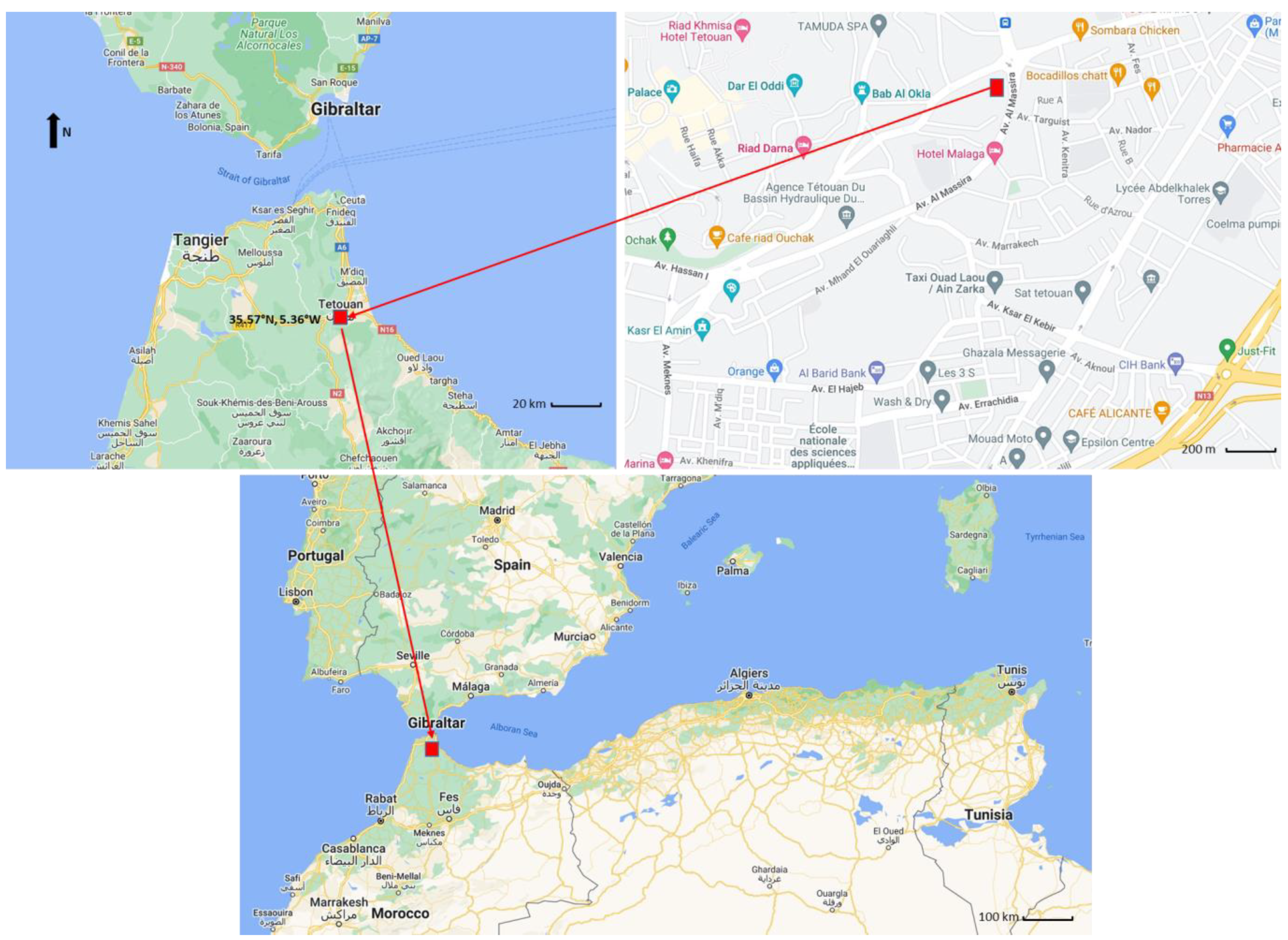
2.1. Sampling and Aerosol Chemical Analyses

For a year, from May 2011 to April 2012, continuous aerosol sampling was conducted in Tetouan city, about 1.5 km west of the historical city center, the Médina (Figure 1). Detailed descriptions of the sampling procedure and analyses of PM₁₀ and PM_2.5 (particulate matter < 10 μm and <2.5 μm in diameter, respectively), elemental carbon (EC), organic carbon (OC), and water-soluble inorganic (WSI) aerosol concentrations were presented in Benchrif et al. [28]. Briefly, each sample of PM₁₀ and PM_2.5 were sampled on 47 mm diameter Teflon filters (Zefluor, Pall Co., Port Washington, WA, USA) for the gravimetric and soluble inorganic ion analyses and 47 mm diameter quartz fiber filters (QM/A, Whatman Inc., Middlesex, UK) for the quantification of the aerosol carbon content. PM cut-off cyclones (model 2000-30ENB, URG Corp., Chapel Hill, NC, USA) operating at 1 m³/h were used for PM₁₀ and PM_2.5 collections. In accordance with EN-12341, PM masses were measured gravimetrically against blank filters under constrained temperature and relative humidity. Loaded and unloaded filters were conditioned for 48 h at below 30% relative humidity before weighing in a Mettler microbalance (UMT3, Mettler Toledo Inc., Greifensee, Switzerland) with 1 μg sensitivity. The PM_coarse (diameters from 2.5 to 10 µm) mass concentrations were calculated by the arithmetic difference of the PM₁₀ and the corresponding PM_2.5 mass concentrations. The uncertainty in the gravimetric measurement was typically of the order of 20 μg, which represents an average uncertainty of 2.0% and 3.8% for PM_2.5 and PM₁₀ measurements, respectively. Filter samples were stored in a dark and cool environment until they were analyzed.

Carbonaceous aerosol (OC and EC) concentrations were analyzed following the two-step combustion protocol developed by Cachier et al. [32]. Uncertainties in the BC and OC measurements corresponded to 4.5% and 7.6%, on average, for our EC and OC mass concentrations. The anions (SO₄²⁻, NO₃⁻, Cl₋, C₂O₄²⁻) and cations (Na⁺, NH₄⁺, K⁺, Mg²⁺, Ca²⁺) were analyzed on a DIONEX^® (model DX-600, Dionex, Sunnyvale, CA, USA) ion chromatograph equipped with a reagent-free system (automated eluent generation and self-regenerating suppression). The concentrations of all ionic species were systematically corrected for procedural blanks which comprised blank filters and analytical reagents. Averaged uncertainty in the analysis of the major inorganic ions was of the order of 10 ppb, which represented less than 1% (0.05 µg/m³) of uncertainty in each atmospheric ion concentration for our field campaign.

The elemental composition analysis in some selected filters was performed for determining the 20 following elements: Al, P, S, Cl, K, Ca, Ti, V, Cr, Mn, Fe, Ni, Cu, Zn, As, Se, Br, Rb, Sr, and Pb. Extracted solutions were analyzed using a total reflection X-ray fluorescence spectrometer (TXRF), model S2-Picofox (Bruker AXS Microanalysis GmbH, Germany). For quantitative analysis, gallium was added as an internal standard to estimate elemental concentrations. After pipetting 10 mL of the digested filter sample onto a siliconized quartz glass carrier and drying under an infrared lamp, the sample was then subjected to a 1000 s TXRF analysis. To track background contamination, a blank filter was analyzed. The blank values were subtracted from the analyzed values. The accuracy of the analysis was assessed using a standard reference material (SRM, 2783 Air particulate on Filter Media-NIST). The relative deviation of the measured concentrations from the reference values ranged from 2 to 14%.

2.2. Aerosol Chemical Closure Methodology

Aerosol chemical closure was achieved using a mass balance methodology based on reconstructed aerosol mass from six representative chemical components, including (1) water-soluble inorganic species or ions; (2) particulate organic matter (POM); (3) black carbon (BC); (4) mineral matter, often referred to as dust material or crustal material; (5) sea salt; and (6) non-determined (nd) or remaining mass, representing other unidentified components. Thus, the reconstructed mass equation takes the following form in Equation (1):

$$m_{reconstructed }={{\displaystyle \sum }}^{ }[m_{BC},m_{POM},m_{ions},m_{dust},m_{salt},m_{nd} ]$$

(1)

Notwithstanding that each component estimated for the reconstruction aerosol mass equation can derive from numerous sources, sprinkling sources often predominate. As reported, for instance, by Chow et al. [14], some fugitive dust sources include salts, which would be included in the salt fraction. However, sulfates and nitrates, which react with salt, would be accounted for in the inorganic ion fraction. Looking beyond merely describing the aerosol mass closure, such a mass balance approach may achieve true closure when the gravimetric mass measurement agrees with the sum of the identified chemical species ($m_{reconstructed}$). The various calculations and assumptions used for the aerosol mass reconstruction are described in the next sections.

• Sea salt component estimation:

The mass of the sea salt is characterized by six major ions: four cations—sodium (ss-Na⁺), magnesium (ss-Mg²⁺), calcium (ss-Ca²⁺), and potassium (ss-K⁺)—and two anions—chloride (ss-Cl⁻) and sulfate (ss-SO₄²⁻) [33]. In the present study, the [Mg²⁺]/[Na⁺] ratio of 0.17 (in both aerosol size fractions) is similar to the one of 0.12 reported by Seinfeld and Pandis [34] for seawater, which suggests that sea spray was the main source for both elements. The obtained results showed good correlations between Na⁺ and Cl⁻ in coarse fraction (r² = 0.76; n = 89), although a poor agreement between our mass ratio [Na⁺]/[Cl⁻] of 1.26 ± 1.41 and the one of 1.8 reported for seawater [34]. Reduction in this ratio as reported by Genga et al. [33] is the consequence of the reaction of acidic gases (primarily nitric and sulphuric acid) with NaCl particles and subsequent volatilization of HCl. This probably means that the marine contribution in this site was aged [35], and it is not possible to use only [NaCl] to describe [sea salt]. Indeed, sea salt concentration may be calculated through the following Equation (2):

[Sea salt] = [Na⁺] + [ss-Cl⁻] + [ss-Mg²⁺] + [ss−K⁺] + [ss−Ca²⁺] + [ss−SO₄²⁻]

(2)

Based on sea water composition, [ss−SO₄²⁻] is estimated as total [Na⁺] times 0.252, [ss-Ca²⁺] as total [Na⁺] times 0.038, [ss-K⁺] as total [Na⁺] times 0.036, sea salt magnesium as total [Na⁺] times 0.12, and [ss-Cl⁻] is calculated as total [Na⁺] times 1.8 [34].

• Inorganic ions:

To estimate contributions from inorganic ions, the sum of non-sea-salt sulfate (nss-SO₄²⁻), NO₃⁻, and NH₄⁺ was estimated [14,36]. Zhang et al. [37] also included K⁺ (a marker for biomass burning) as an additional inorganic ion. The non-sea-salt sulfate (nss-SO₄²⁻) fraction of the total sulfate was estimated by subtracting the fraction of ss-SO₄²⁻ from the total SO₄²⁻. Accordingly, inorganic ion concentration can be calculated as follows in Equation (3):

[inorganic ions] = [nss-SO₄²⁻] + [NO₃⁻] + [NH₄⁺] + [nss-K⁺]

(3)

• Carbonaceous fractions, BC and OC:

BC and OC concentrations were determined in the total quartz filter samples that were collected as discussed before in detail. It is worth noting that, according to Watson et al. [38], BC concentrations and the ratio of OC/BC vary with the carbon analysis method. Moreover, Sciare et al. [39] showed that BC from the thermo-optical method (Sunset Carbon Analyzer Instrument) correlates well with non-sea-salt potassium (nss-K⁺), indicating that it is associated with biomass burning, although BC from the 2-step thermal method [32] is correlated with non-sea-salt sulfate (nss-SO₄²⁻), considered as a tracer for fossil fuel combustion. Here, we shall not attempt to argue for or against whether the influence of the method is contradicted by our findings. Sciare et al. [13] reported that both protocols led to similar chemical mass closure results, whereas the selected carbon analysis protocol for these two methods influenced the BC concentration with a difference on average of 33%. For our case, we have used the concentration obtained from the 2-step thermal method.

• POM calculation:

It is customary to estimate particulate organic matter (POM) concentrations from organic carbon mass by multiplying an OC-to-POM conversion factor (k) derived by measuring the average molecular weight of organic compounds per carbon weight. Turpin and Lim [40] advocated using an OC-to-POM conversion ratio of 1.6 ± 0.2 for urban aerosols and 2.1 ± 0.2 for non-urban (aged or more oxygenated) aerosols. In this work, the calculation of k was performed following Guinot et al.’s [16] methodology. While varying the k from 1.2 to 2.3, the correlation coefficient (r²) between reconstructed (sum of BC, POM, sea salt, mineral dust, and inorganic ion concentrations) and weighed PM_2.5 mass concentration did not change significantly (0.95 < r² < 0.97). Mass closure regression slopes were forced to zero. The correlation coefficient for the scatter plot with the 1.2 conversion factor (i.e., POM = 1.2 × OC) was 0.97, although the slope was 0.88 ± 0.02, implying almost no bias between gravimetric and reconstructed PM_2.5 mass concentrations. In comparison, the use of the k factor of 1.4, usually taken for urban aerosols, overestimated gravimetric PM_2.5 mass with an average of 5%.

• Dust calculation:

Various methods have been used for estimating mineral dust concentrations [16,39,41,42,43]. The widely used equations are documented in Chow et al. [14]. In our samples, dust concentrations were quantified using two approaches suggested by Guinot et al. [16] and Malm et al. [44]. The first chemical closure method was based on reconstructed aerosol mass from BC, OC, ions, Ca²⁺ concentrations, and weighed aerosol mass. It was based on two hypotheses applied separately to the main components of the fine and coarse fractions: (1) The first hypothesis aimed to solve the chemical composition in the fine mode where the particulate organic matter (POM) was the dominant component. The POM content was estimated from the OC-to-POM conversion factor (k) which corresponded to the ratio of organic mass to organic carbon [POM] = k × [OC]. As discussed above, in this study the k factor was estimated to be 1.2. (2) The second hypothesis concerned the coarse mode which was dominated by dust. The mineral dust content was estimated from the Ca²⁺-to-dust conversion factor (f) obtained by performing a linear regression between Ca²⁺ concentration and the missing mass (difference between the reconstructed and weighed mass). The f factor is represented by the slope of this regression, while the intercept accounts for the presence of calcium, nitrate, and/or sulfate in the coarse fraction. Although the aerosol mass concentration in coarse mode (PM_coarse or PM_10–2.5) was estimated through the subtraction of PM_2.5 from collected PM₁₀, large uncertainties for species concentrations were noticed. Then, the application of Guinot et al.’s [16] approach to the calculation above led to a very high chemistry sum compared to the weighed PM_coarse mass. Mineral dust in PM_coarse was then calculated with Malm et al.’s [42] method, as shown in Equation (4):

[mineral dust] = 2.2[Al] + 2.49[Si] + 1.63[Ca] + 1.94[Ti] + 2.42[Fe]

(4)

However, regarding PM_2.5, the conversion factor was, for this study, found to be f = 0.229 and intercept = +1.04, where [mineral dust] = [Ca²⁺]/0.229.

All the elements needed for this equation (Equation (4)), except silica (Si), were determined using total reflection X-ray fluorescence. Silica concentrations were estimated from aluminum following the relationship [Si] = 2.03 × [Al] as reported in Chiapello et al. [45]. In this vein, and for quality assurance purposes, an inter-comparison between ion chromatography (for water-soluble ions) and X-ray fluorescence (for the total elements) analysis results (using logarithmic scales) was carried out as shown in Figure S1. For the analyzed samples dataset, a very good correlation coefficient (r² = 0.92 for PM_2.5 and r² = 0.89 for PM₁₀) and slope (almost 0.8 for both fractions) were obtained.

2.3. Positive Matrix Factorization (PMF) Model

Receptor-based source apportionment techniques have become significant tools for estimating the sources of atmospheric particulate matter (PM) [46,47]. Positive matrix factorization (PMF), one of the receptor models, is a method for modeling PM data based on factor analysis with non-negativity constraints. Thus, the factor elements were constrained as no sample can have a substantially negative factor contribution [20,48,49]. The most important feature of PMF is that it has the potential to integrate variable uncertainties associated with sample measurements. The measured concentrations and the corresponding uncertainties were used for the application of the PMF source apportionment method which can find the primary sources of PM without prior knowledge of the sources. The uncertainty associated with each measured concentration was estimated as the sum of the analysis uncertainty and 1/3 of the detection limit. Values below the detection limit were replaced with half the detection limits and their uncertainties were set at 5/6 of the detection limits. Missing values were replaced by the geometric mean of the measured values and the corresponding uncertainties were set to 4 times this geometric mean [50]. Another important aspect of PMF is the introduction of error estimates (or weights) associated with the input data. This allows problematic data such as outliers or below-detection values to be fed into the model with appropriate weight, avoiding the rejection of such data [49]. The U.S. Environmental Protection Agency (US-EPA) PMF5.0 software [20,51] was used in the current study to achieve the PM source apportionment. Further details of this model have been documented elsewhere [20,45,52,53,54] and are summarized below.

The PMF technique fundamentally resolves the mass balance between the measured species concentrations and source emissions as a linear combination of factors p, species profile f of each source, and the amount of mass g contributed to each sample, according to Equation (5):

$$C_{ij}=\left({{\displaystyle \sum }}_p{g}_{ip} \times f_{pj}\right)+e_{ij}$$

(5)

where C_ij is the concentration of species j measured on sample i, and e_ij is the residual (the difference between the measured value and the value fitted by the model) of the model for the j species measured on sample i. p is the number of factors (sources) that contribute to the measured concentrations. g_ip is the relative contribution of the factor p to the sample i, and f_pj is the concentration of the species j in the factor profile p.

The goal of the model is to find the g_ip, f_pj until a minimum value of the object function Q (Equation (6)) for a given p-value is found. Q is defined as:

$$\mathrm{Q}={{\displaystyle \sum }}_{j=1}^m{{\displaystyle \sum }}_{i=1}^n\left[\frac{e_{ij}^2}{u_{ij}^2}\right]={{\displaystyle \sum }}_{j=1}^m{{\displaystyle \sum }}_{i=1}^n{\left[\frac{C_{ij}-{{\displaystyle \sum }}_{k=1}^p{g}_{ik}\times f_{kj}}{u_{ij}}\right]}^2$$

(6)

where u_ij is the uncertainty of the jth species concentration in sample i, n is the number of samples, and m is the number of species [51].

2.4. Settings and Diagnostics for a PMF Optimum Solution

In the current study, the input database for the PMF source apportionment analysis included 12 chemical elements (BC, OC, Na⁺, NH₄⁺, K⁺, Mg²⁺, Ca²⁺, Cl⁻, NO₃⁻, SO₄²⁻, and C₂O₄²⁻) that were detected in the 89 samples.

Table 1. Input variables and uncertainties used in the EPA PMF 5.0 analyses.

	Carbonaceous Species		Inorganic Ions	Organic Markers
Species	BC	EC	Na+, NH4+, K+, Mg2+, Ca2+, Cl−, NO3−, SO42−	Oxalate	Levoglucosan, Glucose
Uncertainties (µg/m3)	0.15	0.40	0.05	0.01	<0.001

presents the species and their uncertainties used to feed the input dataset for PMF analysis. The three diagnostic tests (bootstrap (BS), displacement (DISP), and bootstrap–displacement (BS-DISP)) offered by PMF 5.0 software were used to evaluate the stability of the solution. Table S1 summarizes the settings and diagnostics used for PMF analysis for PM_2.5 datasets. PM_2.5 mass was set as a total variable to evaluate the contribution of the identified factors to the collected data. All the scaled residuals were between −3.0 and 3.0. Extra modeling uncertainty was adjusted to 20%. No constraints were introduced simultaneously.

Regarding PM_2.5 data, the Qtrue/Qexpected ratio was calculated and found to be 1.27 (i.e., Q theoretical differed by 27% from the Q resulting from the analysis). The BS was run with 400 bootstraps and a minimum correlation r-value of 0.6. BS findings demonstrated that most of the species were well modeled, with a reproducibility of >97% for all factors, while the first factor was mapped in 94% of the runs. The EPA PMF 5.0 user guide suggested that a mapping of bootstrap factors to base factors over 80% indicates that the BS uncertainties can be interpreted, and the number of factors may be appropriate [51]. For a 0.0001 %dQ change and a very low Q decrease (<0.1%), displacement analysis (DISP) revealed no factor swaps. The largest observed drop in Q during DISP was <0.0001%. For the BS-displacement analysis, all relevant variables for factor identification were selected to be displaced, as shown in Table S1. The %dQ change was <0.01%.

Regarding the results of BS mapping, DISP swaps, and BS-DISP analyses, it can be concluded that the best solution for the base run was obtained using five factors with extra modeling uncertainties of 20%. The determination of the optimal number of factors that match significant sources with a physical meaning was achieved by analyzing different parameters as summarized in Table S1. The observed and PMF-modeled PM_2.5 concentrations showed strong correlations (slope = 0.90 and r² = 0.79) indicating a good fit that accurately characterized the real contribution of the PM_2.5 sources in the study area.

3. Results

3.1. Aerosol Chemical Mass Closure

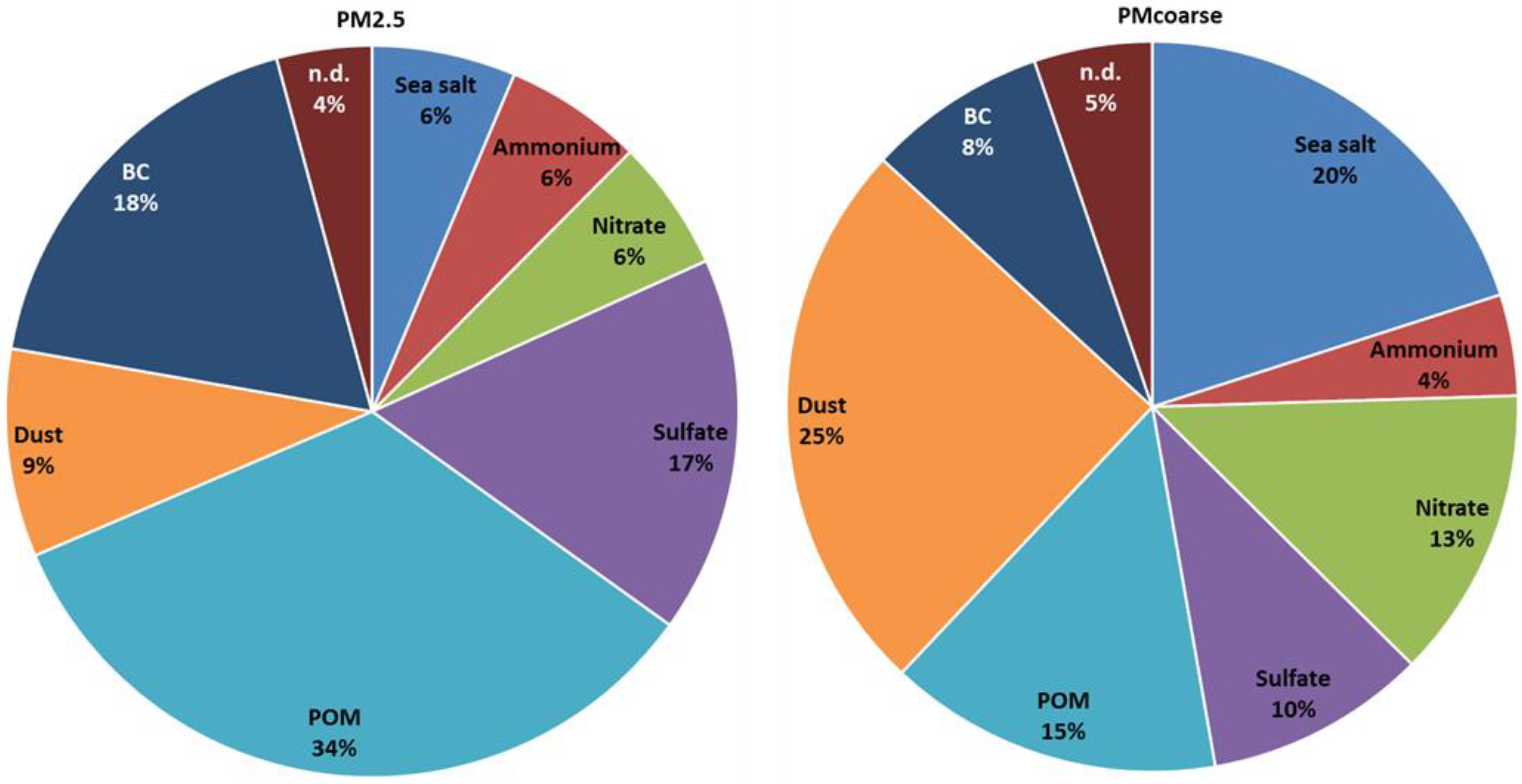
3.1.1. Overview of PM_2.5 and Its Chemical Components

The purpose of this section is to compare the PM_2.5 mass concentration and its major constituents measured in Tetouan city to data obtained from the literature for different locations in the Mediterranean region, as given in

Table 2. Major constituent contributions in % (µg/m³) to PM_2.5. The values are expressed as percentage average (%) while the values in the brackets show the μg/m³. The values for Putaud et al. [58] identified only the average chemical composition (in %) in 14 southern European sites. n.d. stands for the unidentified component; SIA stands for secondary inorganic aerosols (nss-sulfate, nitrate, and ammonium); n.a.: not available; * estimated from the percentage of nss-sulfate; ** nss-sulfate; *** calculated using a conversion factor of 2.1 to convert OC into POM.

	Present Study	14 Southern European Sites [58]	Barcelona (Spain) [57]	Bou-Ismail (Algeria) [11]	Montseny (Spain) [55]	Brindisi Harbor (Italy) [33]	Crete Island (Greece) [39]	Lisbon (Portugal) [8]	Marseille (France) [56]
	May 2011–Apr 2012	1996–2007	2003–2006	2012–2013	2018	Jun–Oct 2012	26 Jul–23 Aug 2001	2001	Jul 2011–Jul 2012
	Urban	Urban	Urban	Rural (Coastal)	Rural	Urban industrial	Background (150 m a.s.l)	Suburban	Urban background
PM2.5	17.96	3–35	29	12.3	5.55	16	17.41	14	19.6
Sea salt	6 (1.14)	6	2 (0.5)	10 (1.36–2.53)	n.a.	3(0.6)	(0.22)	5.4	2.3 (0.33)
Ammonium	6 (1.09)	n.a.	5 (1.4)	5 (1.10)	9 (0.50)	16(2.8)	n.a.	5.7	7.5 (1.5)
Nitrate	6 (1.04)	7	9 (2.7)	4 (1.02)	10 (n.a.)	2(0.3)	(0.07)	6.4	8.5 (1.7)
Sulfate	17 (2.99)	15	16 (4.6)	25 (3.09) *	19 (1.11) **	20(3.6) **	n.a.	18	10.9 (2.2) *
SIA	28 (5.05)	n.a.	30 (8.7)	34 (5.03)	38 (n.a.)	38 (6.7)	(8.06)	30.1	27 (5.4)
POM	34 (6.04)	23	(9)	50 (1.74)	50 (2.83)	33 (6)	(6.13) ***	30	42 (8.6)
Mineral dust	9 (1.65)	11	16 (4.8)	7 (1.52)	7 (0.38)	22 (4)	(0.54)	8.7	19 (n.a.)
BC	18 (3.24)	8	(2.3)	6 (0.83)	3 (0.15)	3 (0.5)	(1.18)	6.8–18	10 (1.8)
n.d.	4 (0.75)	-	18 (5.3)	-	-	1 (0.2)	(1.02)	n.a.	n.a.

. For instance, the PM_2.5 mass concentrations at our sampling site in Tetouan, Morocco, (17.96 µg/m³) were higher than the mean PM_2.5 reported by Veld et al. [55] at a rural site in Montseny, Spain (5.55 µg/m³), observed by Lemou et al. [11] at coastal rural areas in Bou-Ismail, Algeria (12.3 µg/m³), and obtained by Almeida et al. [8] at suburban areas in Lisbon, Portugal (14 µg/m³). It can additionally be noted that the PM_2.5 mass concentrations in Tetouan were in the same range as those obtained at Brindisi harbor (Italy) regarding the prevailing wind direction from an urban industrial area (16 µg/m³) [30], at a background location in Crete (Greece) (17.41 µg/m³) [39], and urban background areas in Marseille (France) (19.6 µg/m³) [56]. Nonetheless, the PM_2.5 mass concentration of our site is largely lower than the values reported by Pérez et al. [57] in urban areas in Barcelona, Spain (29 µg/m³). Putaud et al. [58] stated that PM_2.5 concentrations in most parts of southern Europe range from 3 to 35 µg/m³, while in urban areas they are around 20 µg/m³. Overall, the average PM_2.5 concentrations show a decreasing trend moving from the urban environment to the background atmosphere and then to the suburban and rural environments. These differences emphasize the characteristics of the studied sites and the influenced factors of fine aerosols including, among others, emission sources, meteorological conditions, and air mass trajectory heights and pathways.

At a similar PM_2.5 concentration range measured in this study (16–19 µg/m³), atmospheric particulates were mainly made up of POM in Tetouan (Morocco) (34%, 6.04 µg/m³), Brindisi harbor (Italy) (33%, 6 µg/m³), Crete (France) (6.13 µg/m³), and Marseille (France) (42%, 8.6 µg/m³). Conversely, in Brindisi harbor (Italy), secondary inorganic ions were a major aerosol component (at 33%, 6.7 µg/m³), whereas in Tetouan and Marseille (France) they only made up 29% (6.7 µg/m³) and 27% (5.4 µg/m³) of the PM_2.5 mass, respectively. Another substantial difference between these aerosol mixtures is the contribution of sea salt, which represented 6% (1.14 µg/m³) of the PM_2.5 mass in Tetouan, 2.3% (0.33 µg/m³) in Marseille (France), and 3% (0.6 µg/m³) in Brindisi harbor (Italy). Finally, the mineral dust also showed greater differences between the sites (9%, 3.24 µg/m³ in Tetouan; 22%, 4 µg/m³ in Brindisi harbor; 19% in Marseille; and 0.54 µg/m³ in Crete). Even with distinct rates, POM and SIA were the two main aerosol components, suggesting the dual character of the PM_2.5 origins as local and regional.

In terms of f (Ca²⁺-to-dust) and k (OC-to-POM) conversion factors,

Table 3. Comparison of k (OC-to-POM conversion factor) and f (Ca²⁺-to-dust conversion factor) estimation results with different field experiments. The table is ordered according to k values. * Coarse-mode mass closure efficiency using f; ** fine-mode mass closure efficiency where f fine = f coarse; *** OC-to-POM conversion factor (k) is arbitrarily fixed to 1.8; — data unavailable.

Location	Type	Study Period	Ca2+-to-Dust Conversion Factor, f							OC-to-POM Conversion Factor, k				Reference
			f	Intercept, b	r2	n	% Coarse Closure *	r2	n	k	% Fine Closure **	r2	n
Tetouan, Morocco	Urban	May 2011–Apr 2012	0.229	+1.04	0.52	41	111.8	0.96	51	1.20	95.6	0.97	84	This work
Paris, France	Urban	Jun 2004–Jul 2005	0.150	+0.39	0.67	20	99.7	0.78	20	1.40	99.1	0.89	25	[16]
Florence, Italy	Urban	Jul 2002–Jun 2003	0.120	+0.33	0.56	44	99.6	0.73	46	1.50	97.9	0.85	41	[16]
Gonesse, France	Peri-urban	Sept 2004–Jul 2005	0.072	+0.19	0.90	26	99.3	0.77	26	1.60	98.7	0.86	30	[16]
Beijing, China	Urban	9–27 Aug 2004	0.069–0.085	+0.007–+0.77	0.79–0.98	10–27	99.4–106.7	0.88–0.96	11–24	1.50–1.70	99.0–99.9	0.87–0.99	12–27	[16]
Beijing, China	Urban	10–31 Jan 2003	0.055–0.082	+0.43–+1.07	0.78–0.94	14–29	97.5–99.8	0.85–0.95	20–28	1.55–1.85	99.2–99.6	0.85–0.96	19–28	[16]
Abidjan, Côte d’Ivoire	Urban	Wet season (2015, 2016)	0.015–0.15		0.9	-	-	-	-	1.8 ***	-	-	-	[59]
Abidjan, Côte d’Ivoire	Urban	Dry season (2016, 2017)	0.006–0.07	-	0.9	-				1.8 ***				[59]
Athens, Greece	Urban	16 Mar–19 Apr 2010	-	-	-	-	-	-	-	1.8	73	-	15	[60]

presents the obtained values in the current study compared with former studies at various locations. The determined f and k values are within the range of values provided in the literature. Guinot et al. [16] reported an OC-to-POM ratio of 1.4 for urban (Paris, France) and 1.6 for pre-urban (Florence, Italy) aerosols. Moreover, Adon et al. [59] defined POM at Abidjan (Côte d’Ivoire), an urban African site, as 1.8× OC. The Ca²⁺-to-dust ratio is found to vary in the 0.07–0.20 range in European urban areas, in the 0.007–0.015 range in Abidjan [59], and in a larger range in Beijing (0.07–0.16) [16]. In our case, the OC-to-POM ratio is found to be 1.2, and the f value is of the order of 0.229. Guinot et al. [16] has argued that, for the Beijing experiment, f values reflect competing contributions from long-range transported dust and local dust induced by resuspension. They found that high desert dust influence shifts f to smaller values, whereas significant local dust inputs move f to higher values. Further details on determining the f and k factors are discussed in Section 2.2. In this methodology, the f factor may be addressed as a proxy for mineral dust origin with variations understood as the source signature, while the k factor seems to be a relevant proxy for particle origin and ageing [16]. Thus, the mass closure of fine and coarse aerosol fractions is achieved on average with an efficiency of 96% and 111%, respectively. Figure S2 illustrates the consistency between the weighed and reconstructed masses of PM_2.5 and PM_coarse for the Tetouan experiment. The datasets show that the aerosol mass reconstructed from chemical species masses is largely consistent with the entire mass determined by gravimetric measurements. The difference among PM size fractions and between reconstructed and weighed masses representing the non-determined component (n.d.) is discussed in the next section.

3.1.2. Mass Closure and Differences among PM Size Fractions

Figure 2 depicts the mean picture of the collected particulate matter over the 12 months and the relative abundance of the different components of the identified chemical mass compositions of PM_2.5 and PM_coarse. As shown in Figure 2, the chemical compositions of the two aerosol size fractions are not similar, indicating their different origins and atmospheric lifetimes [61]. All analyzed components are present in both PM_2.5 and PM_coarse but mineral dust and sea salt contribute more to the coarse fraction, whereas POM, BC, and SO₄²⁻ contribute more to the fine fraction. Putaud et al. [62] indicated that PM constituents’ relative contributions to PM mass reflect changes in emission sources and processes that control aerosol compositions. Moreover, aerosols can change their size and chemical composition by the coagulation of particles of different origins and by condensation products resulting from gas-phase reactions [63,64].

The most abundant components in PM_2.5 were POM (34%), BC (18%), and SO₄²⁻ (17%), all adding up to 69% of the mass. In the PM_2.5 fraction, mineral dust still represents a significant component (9%), higher than sea salt (6%), NO₃⁻ (6%,), and NH₄⁺(6%). The estimated PM_coarse is largely dominated by mineral dust (25%) and sea salt (20%), which together account for 45% of the total coarse mass. Remarkably, POM (15%) is a fairly abundant coarse component. This important contribution could be explained by the interaction of mineral dust particles which provide a reactive surface for secondary aerosol formation from the intense anthropogenic group of acidic gas precursors (SO₂, HNO₃, and volatile organic compounds (VOCs)). These interactions favor the formation of a very significant coarse fraction for SO₄, NO₃, and POM [16,65]. NO₃⁻ contribution in the coarse fraction was found to be 13%. Putaud et al. [62] suggested that the presence of sea salt may induce NO₃⁻ to shift towards the aerosol coarse mode. Dasgupta et al. [66] stated that the presence of aerosolized sea salt may enhance the formation of coarse NO₃⁻ in the form of, for example, sodium nitrate (NaNO₃) or calcium nitrate (Ca(NO₃)₂) instead of fine particle ammonium nitrate (NH₄NO₃) or ammonium chloride (NH₄Cl). Further, the pie chart figures provide evidence that sea salt contribution on a yearly basis was about 20% in PM_coarse, while its presence was rarely detected in PM_2.5 (accounting for about 6% of the total mass). This result suggested that sea salt was unlikely to contribute to submicron-sized aerosols.

Lastly, these findings are supported by our previous aerosol transport pathways study [28] which underlined that Tetouan aerosols have mixed origins competing between local carbonaceous aerosols—with a marked contribution from urban and biomass burning sources—and the fresh traffic and maritime vessel aerosols.

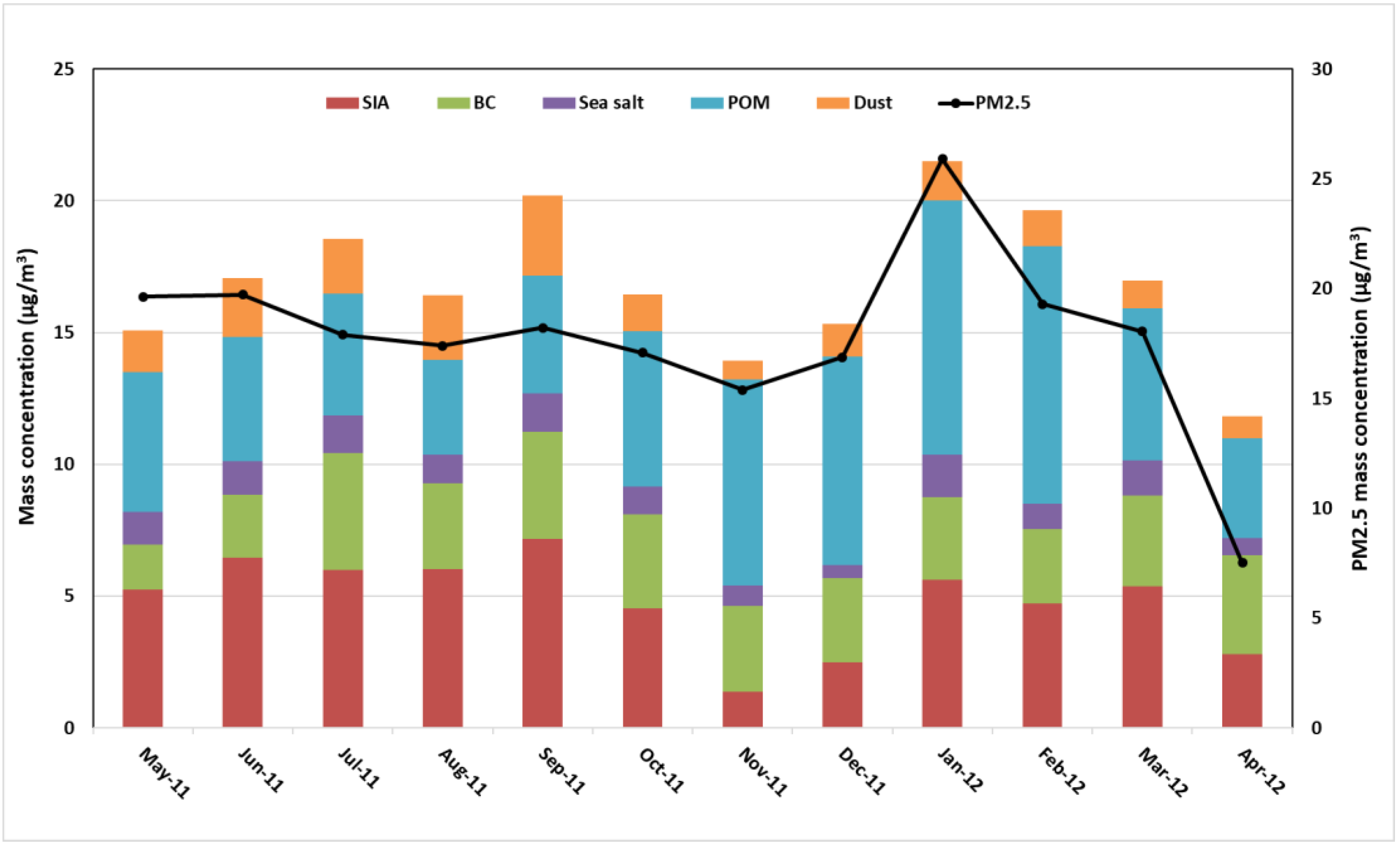
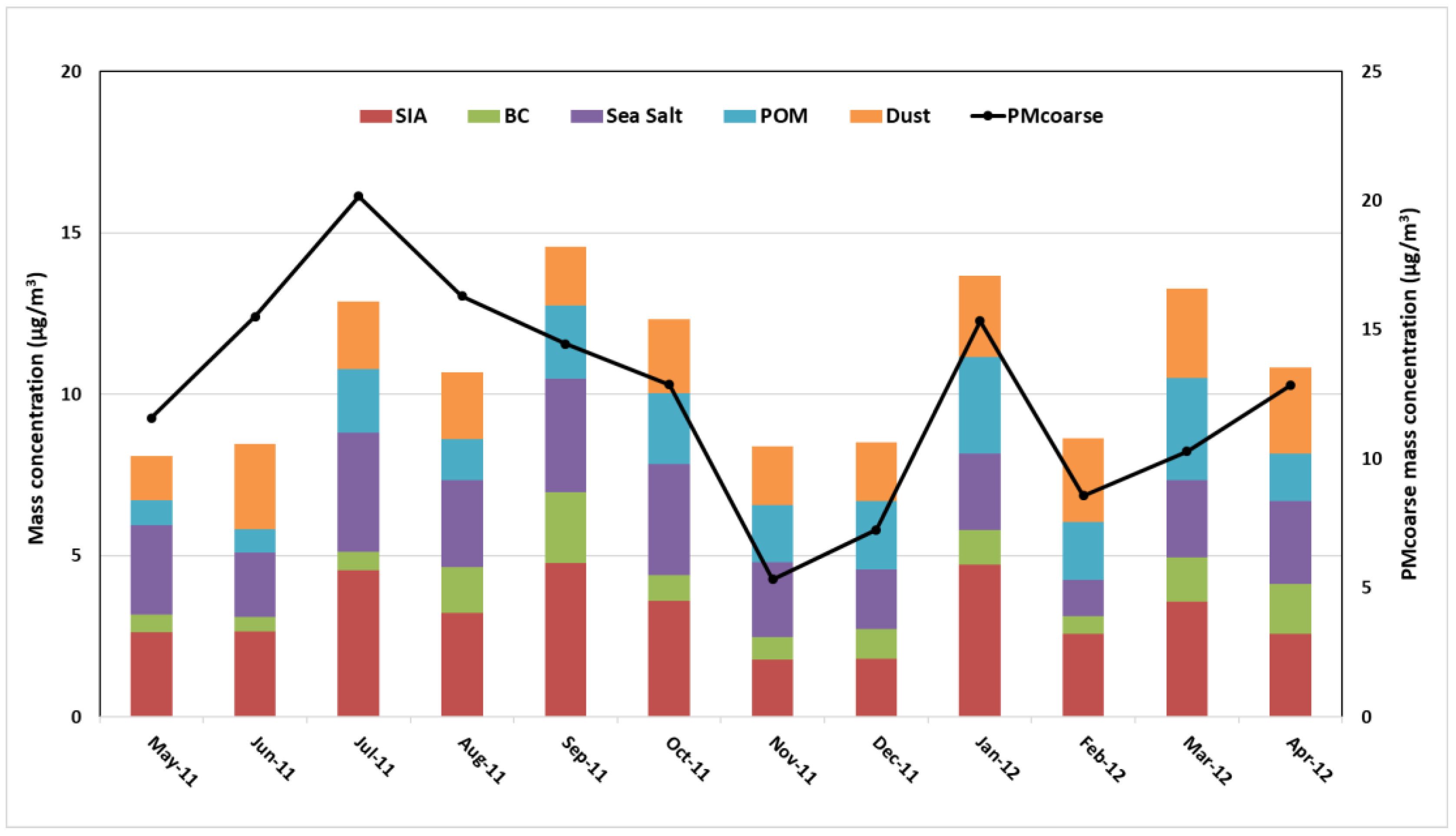
3.1.3. Seasonal Variability of the Reconstructed PM_2.5 and PM_coarse

The outcomes of the mass closure exercise on a monthly basis are shown in Figure 3. Regarding the role of local carbonaceous species found in the fine aerosol fraction of the investigated area, high POM concentrations were observed in January and February, accounting for 9.65 and 9.77 μg/m³, respectively. This abundance of organic matter throughout the October–February cold period was likely due to lower temperatures (Table S3) that favored the aerosol particle phase of organic compounds and low boundary layer heights that induced accumulation of gaseous precursors and acceleration of secondary organic aerosol formation [67]. In addition, seasonal activities can also contribute to the increase in POM in winter. However, significant amounts of mineral dust were registered over the summer period, ranging from 2.07 µg/m³ in July to 3.03 µg/m³ in September. Ion concentrations also show a summer maximum with monthly averages reaching 6.71 and 7.51 μg/m³ in June and September, respectively, indicating a large contribution from photochemistry.

PM_coarse mass concentrations were lower in colder months, which are characterized by high relative humidity and a high ventilation coefficient, as shown in Table S3. Despite the lower PM_coarse mass concentrations, the mineral dust contributions in winter (20%) were similar to or lower than those in spring (20%) and summer (22%). The lowest contribution was recorded during autumn (17%). Furthermore, with a few exceptions during the winter months (December to February) when sea salt concentration (contribution in %) was lower (1.78 µg/m³ (14%) on average), mineral dust (2.32 µg/m³ (20%)) and SIA (3.04 µg/m³ (19%)), including nss-SO₄²⁻, NO₃⁻, and NH₄⁺, were the most abundant species in coarse-mode aerosols. The inorganic aerosol formation was more prevalent in all the summer months, leading to high SIA and dust contributions which averaged 3.74 µg/m³ (24%) and 2.27 µg/m³ (17%), respectively, indicating the significant contribution of the dust matter to the PM_coarse. The contribution of SIA to PM_coarse was 26% on average, with nitrate being the major component (13%). Sea-salt sulfate origins contributed to approximately 5% of the total measured sulfate in this study, which is not included in the SIA category. The highest contribution was in summer, decreasing through autumn and tending to be lowest during winter and spring. Maximum values were observed in September (5.09 µg/m³ on average), whereas the minimum values were in November (1.96 µg/m³) and December (1.86 µg/m³).

3.1.4. Non-Determined Mass

As mentioned earlier, the gravimetric measurements were compared to the reconstructed PM mass concentrations (Figure S2). In the different size fractions, the results were highly correlated, with r² values of 0.96, and 0.97 for PM_2.5, and PM_coarse, respectively. The contributions of the non-determined components ranged from 0.67 to 0.89%. Tian et al. [68] concluded that this contribution increased as the size fractions increased. This unidentified mass is usually attributed to the amount of water associated with aerosol particles [2] and/or to approximations associated with both inorganic species (sulfate and nitrate) and the composition of crustal matter [69], as well as to random and possibly systematic errors [70]. The PM_coarse reconstructed mass is slightly higher than weighed mass because of calculation uncertainties. Thus, according to Sciare et al. [39], the total uncertainties in mass reconstruction derived from chemical analysis can be estimated by error propagation. Accordingly, the obtained relative uncertainty is of the order of 20%.

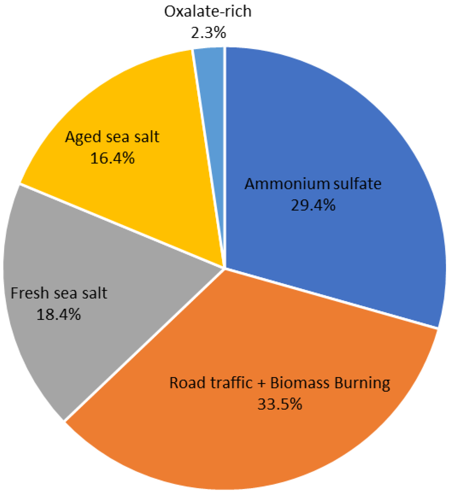
3.2. Source Apportionment of PM_2.5: Source Profiles and Seasonal Variation

As discussed previously, the PMF model was run numerous times with varied factor numbers (4–8) to determine the most physically meaningful solution and the best model diagnostics (Table S1). The Q values, scaled residuals, and consequent source profiles were investigated. Five factors were obtained during the whole year, including: (1) ammonium sulfate, (2) road traffic and biomass burning emissions, (3) fresh sea salt, (4) aged sea salt, and (5) oxalate-rich factors. The PM_2.5 concentrations predicted by the PMF correlated well with the measured ones (slope = 0.90 and r² = 0.79), indicating that the PMF analysis results were reasonably accurate. Figure 4 illustrates the distinguished source profiles, whereas Figure 4 and Figure 5 depict annual average source contributions (in %) from each PMF-resolved source to PM_2.5 mass concentrations and their time variation, respectively. Table S2 show factor profiles (concentration and percentage of species total) obtained from the PMF analysis. Figure S3 presents seasonal mean contributions (in %) of the identified source to PM_2.5 mass concentrations. PMF-resolved sources and their specific tracers are summarized in

Table 4. Summary of PMF-resolved sources and their specific tracers.

Factor	Identified Factors	Specific Tracers
1	Ammonium sulfate	SO42−, NH4+, K+, NO3−
2	Road traffic and biomass burning	OC, BC
3	Fresh sea salt	Cl−, K+, NO3−
4	Aged sea salt	Mg2+, Na+, Ca2+
5	Oxalate-rich factors	Oxalate, NO3−

. The sections that follow discuss each source element and its contributions in detail.

Factor 1 is characterized by high contributions of sulfate (SO₄²⁻), ammonium (NH₄⁺), and potassium (K⁺), which is recommended as a fingerprint for ammonium sulfate [71]. This source constituted as high as 29.4% of the total PM_2.5 mass concentrations on an annual basis, accounting for 5.17 ± 3.94 μg/m³ (Figure 5). The average concentration ratio between SO₄²⁻ and NH₄⁺ in this factor is 2.16, which is consistent with the stoichiometric ratio for ammonium sulfate (i.e., 2.78 by mass). This means that the SO₄²⁻ is mainly in the form of (NH₄)₂SO₄. This factor contains an important contribution from nitrate (32.1%). Manousakas et al. [72] reported that the presence of nitrate (NO₃⁻) in the source profile suggests that this factor is present in general inorganic aerosols rather than exclusively secondary sulfates. In addition, the concentrations of the SO₄²⁻ and NO₃⁻ species show a low correlation (r = 0.37, p-value < 0.0004) as displayed in Figure S4, and they are likely to be apportioned in separate factors (Factor 5). The contributions of this factor were highest during summer (35.7% of total PM_2.5) (Figure 6 and Figure S3), which is quite common for other Mediterranean locations such as Msida station (Malta) [71] and Florence (Italy) [73]. The secondary aerosol component in this factor, sulfate, results from photochemical interactions with atmospheric SO₂, and the enhancement of photochemistry in the warm season favors these reactions [73]. The slow oxidation of SO₂ to SO₄²⁻ led to sulfates being part of aged air masses and hence more associated with transported and regional than local pollution [72].

The road traffic and biomass burning emissions factor (Factor 2) is dominated by high contributions of black carbon (BC, 64.1%) and organic carbon (OC, 64.3%) with the presence of a trace amount of calcium (Ca²⁺, 21.5%) and potassium (K⁺, 19.2%). This factor is found to contribute the most among all the identified factors to the PM_2.5 mass concentrations, accounting for 5.89 ± 3.34 μg/m³ (or 33.5%) of the total PM_2.5 on an annual basis. This factor showed a weak seasonality with clear winter and autumn-high patterns of 32.8% and 29.7%, respectively. The substantial proportion of BC could not be explained by direct emissions from traffic exhausts, which implied that it originated from other combustion sources such as biomass burning, waste burning, and forest fires. However, numerous studies have confirmed that OC and BC were the most abundant species in vehicle exhaust [74,75]. The low OC/BC ratio of 1.81 in the source profile, close to values found in urban areas, such as Milan (1.3) [76] and Metz (1.4) [77], suggests a relatively high contribution from traffic emissions and primary common combustion sources (e.g., combustion and resuspension of combustion particles). For instance, the OC/BC ratio values documented for various European cities showed OC/BC ratios of less than 2 at curbside sites, 2–9 at urban background sites, and increasing with decreasing fresh anthropogenic emissions, reaching values above 10 at rural sites [78,79]. Nevertheless, the presence of K⁺ in this source profile, a strong marker element of biomass burning, indicates possible mixing with other sources including local biomass burning [80]. Since the contributions of K⁺ in the factor profile is low (19.2%), this mixing uncertainty should have had only a minor effect on the estimated factor concentrations. In contrast, 21.5% of Ca²⁺ was apportioned to this factor, implying the contribution of traffic emissions via resuspension of combustion particles. Indeed, Ca²⁺ in an urban setting can arise from a variety of sources, including building activities and global resuspended dust from numerous activities (from biomass burning and traffic) [81]. Since ship emissions have an impact on the Tetouan site, as illustrated in Benchrif et al. [28], we could not rule out the possibility of contributions from shipping emissions. Conversely, the difficulty in identifying accurate sources linked with this factor reflects the fact that, despite the large dataset, distinctive source tracers are lacking in the input data.

The third source factor is assigned as fresh sea salt. It accounts for 18.4% (3.23 ± 3.66 µg/m³) of PM_2.5 mass, with high explained variations for Cl⁻ (89.0%), K⁺ (33.5%), NO₃⁻ (30.7%), and Na⁺ (11.8%). Its significantly higher Cl⁻/Na⁺ ratio (5.7) compared to sea water (1.8) indicates significant ageing, but it still had a substantial contribution from Cl⁻ unlike aged sea salt (discussed in Factor 4 section). Hien et al. [82] stated that a high Cl⁻/Na⁺ ratio suggests that other sources of chloride may have existed but were not resolved by the sea salt factor in the PMF model. It is noteworthy that the sampling site location, somewhat far from the coast (about 10 km), is likely to receive fresh marine contributions. Moreover, this factor also includes NO₃⁻ and OC, accounting for 54.2% of the species sum. The presence of nitrate suggests that sodium nitrate was formed on sea salt particles during aerosol transport from the sea as a consequence of the substitution of chloride by nitrate [83,84]. The contribution from OC in this factor indicates that fresh sea salt is mixed with anthropogenic plumes, while the lack of ammonium indicates that nitrate has been neutralized by sodium. The peak seasonal mass contributions of fresh sea salt sources were seen in the winter (48.0%). This might be linked to high sea breezes or favorable weather conditions for sea salt formation and transport to the study area.

Factor 4 represents aged sea salt. In contrast to fresh sea salt, this factor contributed more to a large number of species—Mg²⁺ (81.7%), Na⁺ (77.8%), and Ca²⁺(54.7%)—in addition to providing a negligible contribution to Cl⁻. The Mg²⁺ to Na⁺ mass concentration ratio was around 0.18, which is very close to the expected value of 0.12 based on sea water composition [34]. In contrast, the observed Cl⁻/Na⁺ ratio of 0.11 differs from the estimated value of 1.8 for fresh sea salt, revealing a strong Cl⁻ shortage compared to the original sea water composition. The observed minimal loadings of chloride in this factor, while sulfate was overabundant, resulted from an ageing process in the atmosphere by acid–base interactions between particulate sea salt and acidic compounds (e.g., nitric and sulfuric acid) [15,77,81]. The high SO₄²⁻/Na⁺ ratio of 2.74 (0.084 in sea water) clearly supports this assumption. This source factor accounted for 16.41% (2.89 ± 2.28 µg/m³) of the total mass of PM_2.5 on an annual scale. A strong seasonality was observed in this factor, with up to 41.3% of the total PM_2.5 mass on average in summer (Figure 6 and Figure S3), which may reflect the seasonality of air mass origins. This latter assumption is supported by a high sulfate/BC ratio (1.4) indicating inputs from sulfur-rich sources, especially from ship emissions. Moreover, Pérez et al. [85] stated that, although sulfate is often associated with regional and long-range transport, its enhanced contributions at an urban site indicate a major intra-urban formation.

One of the originalities of this study is the identification of oxalate-rich factors that have been assumed to be mostly composed of secondary organics. This source factor accounted for 2.3% (0.42 ± 0.44 µg/m³) of the total mass of PM_2.5 on an annual scale. It is dominated by oxalate (91.7%), the most prevalent dicarboxylic acid in the atmosphere, which contributes greatly to secondary organic aerosol [77]. Oxalate can be produced secondarily from photochemical oxidation of anthropogenic, biogenic, and biomass burning emissions [86,87], whereas the primary traffic emissions are reported as low [88]. This factor tended to be higher in the winter months (47.6% of total PM_2.5) than in summer (4.4% of PM_2.5), reflecting the less abundant photochemical production of oxalate in summer. The presence of an amount of NO₃⁻ (23.0%) indicates the contribution of secondary aerosols. A good correlation was found between oxalate and NO₃⁻ in winter (r = 0.72, p-value < 0.00001), providing evidence that vehicular emission was a major secondary source for these two compounds in Tetouan. In fact, the atmospheric precursors of NO₃⁻ and oxalate are among the tracers of vehicular exhausts, namely, NOx and volatile organic matter (VOCs), respectively. In addition, Tetouan aerosol oxalate showed a strong correlation with nss-sulfate in winter (r = 0.84, p-value < 0.03). Jiang et al. [89] argued that the relationships of aerosol oxalate with the two source-indicating species, nss-SO₄²⁻ and NO₃⁻, could provide a hint to the secondary formation pathways of aerosol oxalate. On the other hand, the low correlation between oxalate and K⁺ (r = 0.35, p-value < 0.0004) confirms that the combustion of fossil fuels probably took over biomass burning in the contribution of oxalate in this factor [90]. Further, the average oxalate/K⁺ ratio of 1.19 appeared to be largely higher than the reported values for oxalate measured directly in biomass burning plumes (0.03–0.1) [91], indicating a secondary formation of oxalate.

On the other hand, a noticeable seasonality of the PMF-resolved factor contributions was observed from the previous PMF analyses. With about 48% of the PM_2.5 mass during winter and less than 8% and 5% during summer, the fresh sea salt and oxalate-rich factors, respectively, showed the strongest seasonality among all factors identified (Figure 6 and Figure S3). However, ammonium sulfate and aged sea salt factors can contribute to a significant amount of PM_2.5 during the summer months, with an average contribution of 35.7% and 41.3%, respectively. Conversely, the road traffic and biomass burning factor does not present a clear seasonality pattern.

4. Conclusions

A one-year PM_2.5 chemical characterization and source apportionment study were carried out in the southwestern Mediterranean urban area of Tetouan city, northern Morocco, Chemical characterization was achieved using chemical mass closure calculations for the fine size fraction. The PM_2.5 chemical components were categorized into inorganic ions, particulate organic matter (POM), black carbon (BC), mineral dust, and sea salt. Our findings highlight that Tetouan aerosols have mixed and coexisting sources in which the fine fraction originates primarily from anthropogenic secondary sources. Overall, mass closure exercise reveals that POM (34%), SIA (28%), BC (18%), and to a lesser extent dust (9%) contribute the most to PM_2.5. The typical Ca²⁺-to-dust conversion factor in northern Morocco is estimated to be 0.229, while the ratio of converting organic carbon to particulate organic matter is 1.2. The percentage contribution of POM regarding the fine aerosol mass is in agreement with other study sites in the Mediterranean area, while secondary inorganic aerosols (which were 5.05 µg/m³ on average over the entire campaign) are about a factor of 1.2–1.7 lower.

A comprehensive dataset of chemical analyses was used to estimate the relative contribution of the main PM_2.5 sources with the application of positive matrix factorization (PMF). The modeled and observed PM_2.5 concentrations show high correlations (slope = 0.90 and r² = 0.79) indicating a good fit, which describes well the real contribution of the PM_2.5 sources in the study area. To support the stability of the PMF optimum solution, three diagnostic tests (bootstrap, displacement, and bootstrap–displacement) were completed. One of the originalities of this study is the identification of a factor that is assumed to be mostly composed of secondary organics, recognized here as oxalate-rich factors. PMF analyses identified five source-related factors contributing to PM_2.5 mass at Tetouan, which were named according to their characteristic tracers, including ammonium sulfate (SO₄²⁻, NH₄⁺, K⁺, NO₃⁻), road traffic and biomass burning emissions (OC, BC), fresh sea salt (Cl⁻, K⁺, NO₃⁻), aged sea salt (Mg²⁺, Na⁺, Ca²⁺), and oxalate-rich factors (oxalate, NO₃⁻). We concluded that both the ammonium sulfate and road traffic and biomass burning factors were the dominant sources, representing 62.9% of the PM_2.5, followed by fresh sea salt (18.4%), aged sea salt (16.4%), and oxalate-rich factors (2.4%). A clear seasonality pattern was noticed among the different identified PMF-resolved factors. During the summer months, a high contribution of ammonium sulfate and aged sea salt was observed, together with the road traffic and biomass burning factor from early autumn (September) until winter (end of February). In winter, the fresh sea salt and oxalate-rich factors present important contributions from fresh marine contributions mixed with anthropogenic plumes and secondary aerosols (vehicular exhausts), respectively.

Finally, this study showed that the PMF source apportionment and mass closure results are highly correlated. Both techniques concluded that secondary aerosols such as ammonium sulfate, organics, and black carbon account for the largest drivers of the fine aerosol size fraction in northern Morocco. This indicates that the complementarity of the chemical mass closure and positive matrix factorization is very useful in the identification of emission source contributions for PM_2.5 levels and compositions. Although the identification of distinct seasonal patterns of the source factors was achieved, which could be explained by various sources and meteorological conditions, the objective of a future study could be focused on the parameters influencing the picture of the aerosols of the SW Mediterranean area and their regional or local characteristics in connection with the prevailing meteorological conditions.

References

1. Boucher, O.; Randall, D.; Artaxo, P.; Bretherton, C.; Feingold, G.; Forster, P.; Kerminen, V.-M.; Kondo, Y.; Liao, H.; Lohmann, U.; et al. Clouds and Aerosols. In Climate Change 2013: The Physical Science Basis. Contribution of Working Group I to the Fifth Assessment Report of the Intergovernmental Panel on Climate Change; Stocker, T.F., Qin, D., Plattner, G.-K., Tignor, M., Allen, S.K., Boschung, J., Nauels, A., Xia, Y., Bex, V., Midgley, P.M., Eds.; Cambridge University Press: Cambridge, UK; New York, NY, USA, 2013. [Google Scholar]
2. Terzi, E.; Argyropoulos, G.; Bougatioti, A.; Mihalopoulos, N.; Nikolaou, K.; Samara, C. Chemical composition and mass closure of ambient PM10 at urban sites. Atmos. Environ. 2010, 44, 2231–2239. [Google Scholar] [CrossRef]
3. Niessner, R. Chemical characterization of aerosols. Fresenius J. Anal. Chem. 1990, 337, 565–576. [Google Scholar] [CrossRef]
4. Pey, J.; Querol, X.; Alastuey, A. Variations of levels and composition of PM10 and PM2.5 at an insular site in the Western Mediterranean. Atmos. Res. 2009, 94, 285–299. [Google Scholar] [CrossRef]
5. Rogula-Kozłowska, W.; Klejnowski, K.; Rogula-Kopiec, P.; Ośródka, L.; Krajny, E.; Błaszczak, B.; Mathews, B. Spatial and seasonal variability of the mass concentration and chemical composition of PM2.5 in Poland. Air Qual. Atmos. Health 2013, 7, 41–58. [Google Scholar] [CrossRef] [Green Version]
6. Perrino, C.; Catrambone, M.; Dalla Torre, S.; Rantica, E.; Sargolini, T.; Canepari, S. Seasonal variations in the chemical composition of particulate matter: A case study in the Po Valley. Part I: Macro-components and mass closure. Environ. Sci. Pollut. Res. 2013, 21, 3999–4009. [Google Scholar] [CrossRef]
7. Samara, C.; Kantiranis, N.; Kollias, P.S.; Planou, S.; Kouras, A.; Besis, A.; Manoli, E.; Voutsa, D. Spatial and seasonal variations of the chemical, mineralogical and morphological features of quasi-ultrafine particles (PM0.49) at urban sites. Sci. Total Environ. 2016, 553, 392–403. [Google Scholar] [CrossRef]
8. Almeida, S.M.; Pio, C.; Freitas, M.C.; Reis, M.A.; Trancoso, M.A. Approaching PM2.5 and PM2.5—10 source apportionment by mass balance analysis, principal component analysis and particle size distribution. Sci. Total Environ. 2006, 368, 663–674. [Google Scholar] [CrossRef]
9. Bardouki, H.; Liakakou, H.; Economou, C.; Sciare, J.; Smolík, J.; Zdimal, V.; Eleftheriadis, K.; Lazaridis, M.; Dye, C.; Mihalopoulos, N. Chemical composition of size-resolved atmospheric aerosols in the eastern Mediterranean during summer and winter. Atmos. Environ. 2003, 37, 195–208. [Google Scholar] [CrossRef]
10. Clemente, Á.; Yubero, E.; Galindo, N.; Crespo, J.; Nicolás, J.F.; Santacatalina, M.; Carratalá, A. Quantification of the impact of port activities on PM10 levels at the port-city boundary of a mediterranean city. J. Environ. Manag. 2020, 281, 111842. [Google Scholar] [CrossRef]
11. Lemou, A.; Rabhi, L.; Merabet, H.; Ladji, R.; Nicolas, J.B.; Bonnaire, N.; Mustapha, M.A.; Dilmi, R.; Sciare, J.; Mihalopoulos, N.; et al. Chemical characterization of fine particles (PM2.5) at a coastal site in the South Western Mediterranean during the ChArMex experiment. Environ. Sci. Pollut. Res. 2020, 27, 20427–20445. [Google Scholar] [CrossRef]
12. Perrino, C.; Catrambone, M.; Farao, C.; Canepari, S. Assessing the contribution of water to the mass closure of PM10. Atmos. Environ. 2016, 140, 555–564. [Google Scholar] [CrossRef]
13. Sciare, J.; Cachier, H.; Oikonomou, K.; Ausset, P.; Sarda-Estève, R.; Mihalopoulos, N. Characterization of carbonaceous aerosols during the MINOS campaign in Crete, July–August 2001: A multi-analytical approach. Atmos. Chem. Phys. 2003, 3, 1743–1757. [Google Scholar] [CrossRef] [Green Version]
14. Chow, J.C.; Lowenthal, D.H.; Chen, L.A.; Wang, X.; Watson, J.G. Mass reconstruction methods for PM2.5: A review. Air Qual. Atmos. Health 2015, 8, 243–263. [Google Scholar] [CrossRef] [Green Version]
15. Masiol, M.; Squizzato, S.; Formenton, G.; Khan, M.B.; Hopke, P.K.; Nenes, A.; Pandis, S.N.; Tositti, L.; Benetello, F.; Visin, F.; et al. Hybrid multiple-site mass closure and source apportionment of PM2.5 and aerosol acidity at major cities in the Po Valley. Sci. Total Environ. 2020, 704, 135287. [Google Scholar] [CrossRef]
16. Guinot, B.; Cachier, H.; Oikonomou, K. Geochemical perspectives from a new aerosol chemical mass closure. Atmos. Chem. Phys. 2006, 7, 1657–1670. [Google Scholar] [CrossRef] [Green Version]
17. Naila, S.; Shahida, W. Source apportionment using reconstructed mass calculations. J. Environ. Sci. Health Part A Toxic/Hazard. Subst. Environ. Eng. 2014, 49, 463–477. [Google Scholar] [CrossRef]
18. Belis, C.A.; Favez, O.; Mircea, M.; Diapouli, E.; Manousakas, M.-I.; Vratolis, S.; Gilardoni, S.; Paglione, M.; Decesari, S.; Mocnik, G.; et al. European Guide on Air Pollution Source Apportionment with Receptor Models—Revised Version 2019; EUR 29816 EN; Publications Office of the European Union: Luxembourg, 2019. [Google Scholar] [CrossRef]
19. Diapouli, E.; Manousakas, M.I.; Vratolis, S.; Vasilatou, V.; Pateraki, S.; Bairachtari, K.A.; Querol, X.; Amato, F.; Alastuey, A.; Karanasiou, A.; et al. AIRUSE-LIFE +: Estimation of natural source contributions to urban ambient air PM 10 and PM 2. 5 concentrations in southern Europe—Implications to compliance with limit values. Atmos. Chem. Phys. 2016, 17, 3673–3685. [Google Scholar] [CrossRef] [Green Version]
20. Paatero, P.; Eberly, S.I.; Brown, S.; Norris, G.A. Methods for estimating uncertainty in factor analytic solutions. Atmos. Meas. Technol. 2014, 7, 781–797. [Google Scholar] [CrossRef] [Green Version]
21. Souto-Oliveira, C.E.; Kamigauti, L.Y.; Andrade, M.D.; Babinski, M. Improving Source Apportionment of Urban Aerosol Using Multi-Isotopic Fingerprints (MIF) and Positive Matrix Factorization (PMF): Cross-Validation and New Insights. Front. Environ. Sci. 2021, 9, 623915. [Google Scholar] [CrossRef]
22. Bove, M.C.; Massabò, D.; Prati, P. PMF5.0 vs. CMB8.2: An inter-comparison study based on the new European SPECIEUROPE database. Atmos. Res. 2018, 201, 181–188. [Google Scholar] [CrossRef]
23. Merabet, H.; Kerbachi, R.; Mihalopoulos, N.; Stavroulas, I.; Kanakidou, M.; Yassaa, N. Measurement of atmospheric black carbon in some South Mediterranean cities. Clean Air J. 2019, 29, 1–19. [Google Scholar] [CrossRef] [Green Version]
24. Dammak, R.; Chabbi, I.; Bahloul, M.; Azri, C. PM10 temporal variation and multi-scale contributions of sources and meteorology in Sfax, Tunisia. Air Qual. Atmos. Health 2020, 13, 617–628. [Google Scholar] [CrossRef]
25. Abu-Allaban, M.M.; Lowenthal, D.H.; Gertler, A.W.; Labib, M. Sources of PM10 and PM2.5 in Cairo’s ambient air. Environ. Monit. Assess. 2007, 133, 417–425. [Google Scholar] [CrossRef]
26. Khedidji, S.; Müller, K.; Rabhi, L.; Spindler, G.; Fomba, K.W.; Pinxteren, D.V.; Yassaa, N.; Herrmann, H. Chemical Characterization of Marine Aerosols in a South Mediterranean Coastal Area Located in Bou Ismaïl, Algeria. Aerosol Air Qual. Res. 2020, 20, 2448–2473. [Google Scholar] [CrossRef]
27. Saad, M.H.; Masmoudi, M.M.; Chevaillier, S.; Laurent, B.; Lafon, S.; Alfaro, S.C. Variability of the elemental composition of airborne mineral dust along the coast of Central Tunisia. Atmos. Res. 2018, 209, 170–178. [Google Scholar] [CrossRef]
28. Benchrif, A.; Guinot, B.; Bounakhla, M.; Cachier, H.; Damnati, B.; Baghdad, B. Aerosols in Northern Morocco: Input pathways and their chemical fingerprint. Atmos. Environ. 2018, 174, 140–147. [Google Scholar] [CrossRef]
29. Metternich, P.; Georgii, H.; Groeneveld, K.O. Long range transport of atmospheric aerosol particles over the Mediterranean and Atlantic Ocean. Nucl. Instrum. Methods Phys. Res. Sect. B-Beam Interact. Mater. At. 1984, 3, 475–478. [Google Scholar] [CrossRef]
30. Al-Momani, I.; Güllü, G.; Ölmez, I.; Eler, Ü.; Örtel, E.; Şirin, G.; Tuncel, G. Chemical composition of eastern Mediterranean aerosol and precipitation: Indications of long-range transport. Pure Appl. Chem. 1997, 69, 41–46. [Google Scholar] [CrossRef]
31. Ancellet, G.; Pelon, J.; Totems, J.; Chazette, P.; Bazureau, A.; Sicard, M.; Iorio, T.D.; Dulac, F.; Mallet, M.D. Long range transport and mixing of aerosol sources during the 2013 North American biomass burning episode: Analysis of multiple lidar observations in the Western Mediterranean basin. Atmos. Chem. Phys. 2015, 16, 4725–4742. [Google Scholar] [CrossRef]
32. Cachier, H.; Bremond, M.P.; Buat-Ménard, P. Determination of atmospheric soot carbon with a simple thermal method. Tellus B 1989, 41, 379–390. [Google Scholar] [CrossRef] [Green Version]
33. Genga, A.; Ielpo, P.; Siciliano, T.; Siciliano, M. Carbonaceous particles and aerosol mass closure in PM2.5 collected in a port city. Atmos. Res. 2017, 183, 245–254. [Google Scholar] [CrossRef]
34. Seinfeld, J.H.; Pandis, S.N. Atmospheric Chemistry and Physics: From Air Pollution to Climate Change; Wiley: Hoboken, NJ, USA, 1997. [Google Scholar] [CrossRef]
35. Cesari, D.; Genga, A.; Ielpo, P.; Siciliano, M.; Mascolo, G.; Grasso, F.M.; Contini, D. Source apportionment of PM(2.5) in the harbour-industrial area of Brindisi (Italy): Identification and estimation of the contribution of in-port ship emissions. Sci. Total Environ. 2014, 497–498, 392–400. [Google Scholar] [CrossRef] [PubMed]
36. Cheung, K.; Daher, N.; Kam, W.; Shafer, M.M.; Ning, Z.; Schauer, J.J.; Sioutas, C. Spatial and temporal variation of chemical composition and mass closure of ambient coarse particulate matter (PM10-2.5) in the Los Angeles area. Atmos. Environ. 2011, 45, 2651–2662. [Google Scholar] [CrossRef]
37. Zhang, Y.; Sartelet, K.; Zhu, S.; Wang, W.; Wu, S.Y.; Zhang, X.; Wang, K.; Tran, P.; Seigneur, C.; Wang, Z. Application of WRF/Chem-MADRID and WRF/Polyphemus in Europe—Part 2: Evaluation of chemical concentrations and sensitivity simulations. Atmos. Chem. Phys. 2013, 13, 6845–6875. [Google Scholar] [CrossRef] [Green Version]
38. Watson, J.G.; Chow, J.C.; Chen, L.A. Summary of Organic and Elemental Carbon/Black Carbon Analysis Methods and Intercomparisons. Aerosol Air Qual. Res. 2005, 5, 65–102. [Google Scholar] [CrossRef] [Green Version]
39. Sciare, J.; Oikonomou, K.; Cachier, H.; Mihalopoulos, N.; Andreae, M.O.; Maenhaut, W.; Sarda-Estève, R. Aerosol mass closure and reconstruction of the light scattering coefficient over the Eastern Mediterranean Sea during the MINOS campaign. Atmos. Chem. Phys. 2005, 5, 2253–2265. [Google Scholar] [CrossRef] [Green Version]
40. Turpin, B.J.; Lim, H. Species Contributions to PM2.5 Mass Concentrations: Revisiting Common Assumptions for Estimating Organic Mass. Aerosol Sci. Technol. 2001, 35, 602–610. [Google Scholar] [CrossRef]
41. Guieu, C.; Loÿe-Pilot, M.; Ridame, C.; Thomas, C. Chemical characterization of the Saharan dust end-member: Some biogeochemical implications for the western Mediterranean Sea. J. Geophys. Res. 2002, 107, 4258. [Google Scholar] [CrossRef]
42. Malm, W.C.; Sisler, J.F.; Huffman, D.; Eldred, R.A.; Cahill, T.A. Spatial and seasonal trends in particle concentration and optical extinction in the United States. J. Geophys. Res. 1994, 99, 1347–1370. [Google Scholar] [CrossRef]
43. Chow, J.C.; Watson, J.G.; Fujita, E.M.; Lu, Z.; Lawson, D.R.; Ashbaugh, L.L. Temporal and spatial variations of PM2.5 and PM10 aerosol in the Southern California air quality study. Atmos. Environ. 1994, 28, 2061–2080. [Google Scholar] [CrossRef]
44. Malm, W.C.; Schichtel, B.A.; Pitchford, M.L. Uncertainties in PM2.5 Gravimetric and Speciation Measurements and What We Can Learn from Them. J. Air Waste Manag. Assoc. 2011, 61, 1131–1149. [Google Scholar] [CrossRef] [PubMed] [Green Version]
45. Chiapello, I.; Bergametti, G.; Châtenet, B.; Bousquet, P.; Dulac, F.; Soares, E.S. Origins of African dust transported over the northeastern tropical Atlantic. J. Geophys. Res. 1997, 102, 13701–13709. [Google Scholar] [CrossRef] [Green Version]
46. Kelly, K.E.; Kotchenruther, R.; Kuprov, R.; Silcox, G.D. Receptor model source attributions for Utah’s Salt Lake City airshed and the impacts of wintertime secondary ammonium nitrate and ammonium chloride aerosol. J. Air Waste Manag. Assoc. 2013, 63, 575–590. [Google Scholar] [CrossRef] [PubMed] [Green Version]
47. Tian, Y.; Shi, G.; Han, B.; Wang, W.; Zhou, X.; Wang, J.; Li, X.; Feng, Y. The accuracy of two- and three-way positive matrix factorization models: Applying simulated multisite data sets. J. Air Waste Manag. Assoc. 2014, 64, 1122–1129. [Google Scholar] [CrossRef] [Green Version]
48. Paatero, P.; Tapper, U. Positive matrix factorization: A non-negative factor model with optimal utilization of error estimates of data values. Environmetrics 1994, 5, 111–126. [Google Scholar] [CrossRef]
49. Sara, C.; Luisa, C.; Bernd, G. Positive Matrix Factorisation (PMF)—An Introduction to the Chemometric Evaluation of Environmental Monitoring Data Using PMF; Joint Research Centre: Brussels, Belgium, 2009. [Google Scholar] [CrossRef]
50. Kim, E.; Hopke, P.K. Improving source identification of fine particles in a rural northeastern U.S. area utilizing temperature-resolved carbon fractions. J. Geophys. Res. 2004, 109, D09204. [Google Scholar] [CrossRef]
51. Norris, G.; Duvall, R.; Brown, S.; Bai, S. EPA Positive Matrix Factorization (PMF) 5.0 Fundamentals and User Guide; Technical Report; U.S. Environmental Protection Agency, National Exposure Research Laboratory: Washington, DC, USA, 2014.
52. Brown, S.G.; Eberly, S.I.; Paatero, P.; Norris, G.A. Methods for estimating uncertainty in PMF solutions: Examples with ambient air and water quality data and guidance on reporting PMF results. Sci. Total Environ. 2015, 518–519, 626–635. [Google Scholar] [CrossRef]
53. Farahmandkia, Z.; Moattar, F.; Zayeri, F.; Sadegh Sekhavatjou, M.; Mansouri, N. Contribution of point and small-scaled sources to the PM10 emission using positive matrix factorization model. J. Environ. Health Sci. Eng. 2017, 15, 2. [Google Scholar] [CrossRef] [PubMed] [Green Version]
54. Weber, S.; Salameh, D.; Albinet, A.; Alleman, L.Y.; Waked, A.; Besombes, J.L.; Jacob, V.; Guillaud, G.; Meshbah, B.; Rocq, B.; et al. Comparison of PM10 Sources Profiles at 15 French Sites Using a Harmonized Constrained Positive Matrix Factorization Approach. Atmosphere 2019, 10, 310. [Google Scholar] [CrossRef] [Green Version]
55. Veld, M.I.; Alastuey, A.; Pandolfi, M.; Amato, F.; Pérez, N.; Reche, C.; Via, M.; Minguillón, M.C.; Escudero, M.; Querol, X. Compositional changes of PM2.5 in NE Spain during 2009–2018: A trend analysis of the chemical composition and source apportionment. Sci. Total Environ. 2021, 795, 148728. [Google Scholar] [CrossRef] [PubMed]
56. Salameh, D.; Detournay, A.; Pey, J.; Pérez, N.; Liguori, F.; Saraga, D.; Bove, M.C.; Brotto, P.; Cassola, F.; Massabò, D.; et al. PM2.5 chemical composition in five European Mediterranean cities: A 1-year study. Atmos. Res. 2015, 155, 102–117. [Google Scholar] [CrossRef]
57. Pérez, N.; Pey, J.; Querol, X.; Alastuey, A.; López, J.M.; Viana, M. Partitioning of major and trace components in PM10–PM2.5–PM1 at an urban site in Southern Europe. Atmos. Environ. 2008, 42, 1677–1691. [Google Scholar] [CrossRef]
58. Putaud, J.; Dingenen, R.V.; Alastuey, A.; Bauer, H.; Birmili, W.; Cyrys, J.; Flentje, H.E.; Fuzzi, S.; Gehrig, R.; Hansson, H.; et al. A European aerosol phenomenology 3: Physical and chemical characteristics of particulate matter from 60 rural, urban, and kerbside sites across Europe. Atmos. Environ. 2010, 44, 1308–1320. [Google Scholar] [CrossRef]
59. Adon, A.J.; Liousse, C.; Doumbia, E.H.; Baeza-Squiban, A.; Cachier, H.; Léon, J.F.; Yoboué, V.; Akpo, A.B.; Galy-Lacaux, C.; Guinot, B.; et al. Physico-chemical characterization of urban aerosols from specific combustion sources in West Africa at Abidjan in Côte d’Ivoire and Cotonou in Benin in the frame of the DACCIWA program. Atmos. Chem. Phys. 2020, 20, 5327–5354. [Google Scholar] [CrossRef]
60. Remoundaki, E.; Kassomenos, P.A.; Mantas, E.; Mihalopoulos, N.; Tsezos, M. Composition and Mass Closure of PM2.5 in Urban Environment (Athens, Greece). Aerosol Air Qual. Res. 2013, 13, 72–82. [Google Scholar] [CrossRef] [Green Version]
61. Rogula-Kozłowska, W.; Klejnowski, K.; Rogula-Kopiec, P.; Mathews, B.; Szopa, S. A Study on the Seasonal Mass Closure of Ambient Fine and Coarse Dusts in Zabrze, Poland. Bull. Environ. Contam. Toxicol. 2012, 88, 722–729. [Google Scholar] [CrossRef] [PubMed]
62. Putaud, J.P.; Raes, F.; Van Dingenen, R.; Brüggemann, E.; Facchini, M.C.; Decesari, S.; Fuzzi, S.; Gehrig, R.; Hüglin, C.; Laj, P.; et al. A european aerosol phenomenology—2: Chemical characteristics of particulate matter at kerbside, urban, rural and background sites in Europe. Atmos. Environ. 2004, 38, 2579–2595. [Google Scholar] [CrossRef]
63. Myhre, G.; Myhre, C.E.L.; Samset, B.H.; Storelvmo, T. Aerosols and their Relation to Global Climate and Climate Sensitivity. Nat. Educ. Knowl. 2013, 4, 7. [Google Scholar]
64. Hidy, G.M. Chapter 7—Atmospheric Aerosols. In Aerosols; Academic Press: Cambridge, MA, USA, 1984. [Google Scholar] [CrossRef]
65. Babar, Z.B.; Park, J.; Lim, H. Influence of NH 3 on secondary organic aerosols from the ozonolysis and photooxidation of α-pinene in a flow reactor. Atmos. Environ. 2017, 164, 71–84. [Google Scholar] [CrossRef]
66. Dasgupta, P.K.; Campbell, S.W.; Al-Horr, R.S.; Ullah, S.M.; Li, J.; Amalfitano, C.; Poor, N.D. Conversion of sea salt aerosol to NaNO3 and the production of HCl: Analysis of temporal behavior of aerosol chloride/nitrate and gaseous HCl/HNO3 concentrations with AIM. Atmos. Environ. 2007, 41, 4242–4257. [Google Scholar] [CrossRef]
67. Vecchi, R.; Chiari, M.; D’Alessandro, A.; Fermo, P.; Lucarelli, F.; Mazzei, F.; Nava, S.; Piazzalunga, A.; Prati, P.; Silvani, F.; et al. A mass closure and PMF source apportionment study on the sub-micron sized aerosol fraction at urban sites in Italy. Atmos. Environ. 2008, 42, 2240–2253. [Google Scholar] [CrossRef]
68. Tian, S.; Pan, Y.; Wang, Y. Size-resolved source apportionment of particulate matter in urban Beijing during haze and non-haze episodes. Atmos. Chem. Phys. 2016, 16, 1–19. [Google Scholar] [CrossRef] [Green Version]
69. Speer, R.E.; Edney, E.O.; Kleindienst, T.E. Impact of organic compounds on the concentrations of liquid water in ambient PM2.5. J. Aerosol Sci. 2003, 34, 63–77. [Google Scholar] [CrossRef]
70. Dingenen, R.V.; Raes, F.; Putaud, J.; Baltensperger, U.; Charron, A.; Facchini, M.C.; Decesari, S.; Fuzzi, S.; Gehrig, R.; Hansson, H.; et al. A European aerosol phenomenology-1: Physical characteristics of particulate matter at kerbside, urban, rural and background sites in Europe. Atmos. Environ. 2004, 38, 2561–2577. [Google Scholar] [CrossRef]
71. Scerri, M.; Kandler, K.; Weinbruch, S.; Yubero, E.; Galindo, N.; Prati, P.; Caponi, L.; Massabò, D. Estimation of the contributions of the sources driving PM2.5 levels in a Central Mediterranean coastal town. Chemosphere 2018, 211, 465–481. [Google Scholar] [CrossRef] [PubMed]
72. Manousakas, M.; Papaefthymiou, H.; Diapouli, E.; Migliori, A.; Karydas, A.G.; Bogdanović-Radović, I.; Eleftheriadis, K. Assessment of PM2.5 sources and their corresponding level of uncertainty in a coastal urban area using EPA PMF 5.0 enhanced diagnostics. Sci. Total Environ. 2017, 574, 155–164. [Google Scholar] [CrossRef] [PubMed] [Green Version]
73. Nava, S.; Calzolai, G.; Chiari, M.; Giannoni, M.; Giardi, F.; Becagli, S.; Severi, M.; Traversi, R.; Lucarelli, F. Source Apportionment of PM2.5 in Florence (Italy) by PMF Analysis of Aerosol Composition Records. Atmosphere 2020, 11, 484. [Google Scholar] [CrossRef]
74. Wang, Y.; Jia, C.; Tao, J.; Zhang, L.; Liang, X.; Ma, J.; Gao, H.; Huang, T.; Zhang, K. Chemical characterization and source apportionment of PM2.5 in a semi-arid and petrochemical-industrialized city, Northwest China. Sci. Total Environ. 2016, 573, 1031–1040. [Google Scholar] [CrossRef]
75. Tan, J.; Zhang, L.; Zhou, X.; Duan, J.; Li, Y.; Hu, J.; He, K. Chemical characteristics and source apportionment of PM2.5 in Lanzhou, China. Sci. Total Environ. 2017, 601–602, 1743–1752. [Google Scholar] [CrossRef]
76. Lonati, G.; Giugliano, M.; Butelli, P.; Romele, L.; Tardivo, R. Major chemical components of PM2.5 in Milan (Italy). Atmos. Environ. 2005, 39, 1925–1934. [Google Scholar] [CrossRef]
77. Petit, J.; Pallarès, C.; Favez, O.; Alleman, L.Y.; Bonnaire, N.; Rivière, E.D. Sources and Geographical Origins of PM10 in Metz (France) Using Oxalate as a Marker of Secondary Organic Aerosols by Positive Matrix Factorization Analysis. Atmosphere 2019, 10, 370. [Google Scholar] [CrossRef] [Green Version]
78. Samara, C.; Voutsa, D.; Kouras, A.; Eleftheriadis, K.; Maggos, T.; Saraga, D.E.; Petrakakis, M.J. Organic and elemental carbon associated to PM10 and PM2.5 at urban sites of northern Greece. Environ. Sci. Pollut. Res. 2013, 21, 1769–1785. [Google Scholar] [CrossRef] [PubMed]
79. Manousakas, M.I.; Florou, K.; Pandis, S.N. Source Apportionment of Fine Organic and Inorganic Atmospheric Aerosol in an Urban Background Area in Greece. Atmosphere 2020, 11, 330. [Google Scholar] [CrossRef] [Green Version]
80. Jeong, C.; Herod, D.; Dabek-Złotorzyńska, E.; Ding, L.C.; McGuire, M.L.; Evans, G.J. Identification of the sources and geographic origins of black carbon using factor analysis at paired rural and urban sites. Environ. Sci. Technol. 2013, 47, 8462–8470. [Google Scholar] [CrossRef] [PubMed]
81. Borlaza, L.J.; Weber, S.; Uzu, G.; Jacob, V.; Cañete, T.; Micallef, S.; Trébuchon, C.; Slama, R.; Favez, O.; Jaffrezo, J.L. Disparities in particulate matter (PM10) origins and oxidative potential at a city scale (Grenoble, France)—Part 1: Source apportionment at three neighbouring sites. Atmos. Chem. Phys. 2021, 21, 5415–5437. [Google Scholar] [CrossRef]
82. Hien, P.D.; Bac, V.T.; Thinh, N.T.; Anh, H.L.; Thang, D.D.; Nghia, N.T. A Comparison Study of Chemical Compositions and Sources of PM1.0 and PM2.5 in Hanoi. Aerosol Air Qual. Res. 2021, 21, 210056. [Google Scholar] [CrossRef]
83. Pathak, R.; Yao, X.; Lau, A.K.H.; Chan, C.K. Acidity and concentrations of ionic species of PM2.5 in Hong Kong. Atmos. Environ. 2003, 37, 1113–1124. [Google Scholar] [CrossRef]
84. Crilley, L.R.; Lucarelli, F.; Bloss, W.J.; Harrison, R.M.; Beddows, D.C.; Calzolai, G.; Nava, S.; Valli, G.; Bernardoni, V.; Vecchi, R. Source apportionment of fine and coarse particles at a roadside and urban background site in London during the 2012 summer ClearfLo campaign. Environ. Pollut. 2017, 220, 766–778. [Google Scholar] [CrossRef] [Green Version]
85. Pérez, N.; Pey, J.; Reche, C.; Cortés, J.; Alastuey, A.; Querol, X. Impact of harbour emissions on ambient PM10 and PM2.5 in Barcelona (Spain): Evidences of secondary aerosol formation within the urban area. Sci. Total Environ. 2016, 571, 237–250. [Google Scholar] [CrossRef]
86. Martinelango, P.; Dasgupta, P.K.; Al-Horr, R.S. Atmospheric production of oxalic acid/oxalate and nitric acid/nitrate in the Tampa Bay airshed: Parallel pathways. Atmos. Environ. 2007, 41, 4258–4269. [Google Scholar] [CrossRef]
87. Xing, L.; Fu, T.; Cao, J.J.; Lee, S.; Wang, G.; Ho, K.F.; Cheng, M.; You, C.; Wang, T. Seasonal and spatial variability of the OM/OC mass ratios and high regional correlation between oxalic acid and zinc in Chinese urban organic aerosols. Atmos. Chem. Phys. 2013, 13, 4307–4318. [Google Scholar] [CrossRef] [Green Version]
88. Huang, X.; Yu, J. Is vehicle exhaust a significant primary source of oxalic acid in ambient aerosols? Geophys. Res. Lett. 2007, 34, L02808. [Google Scholar] [CrossRef]
89. Jiang, Y.; Zhuang, G.; Wang, Q.; Liu, T.; Huang, K.; Fu, J.S.; Li, J.; Lin, Y.; Zhang, R.; Deng, C. Characteristics, sources and formation of aerosol oxalate in an Eastern Asia megacity and its implication to haze pollution. Atmos. Chem. Phys. Discuss. 2011, 11, 22075–22112. [Google Scholar] [CrossRef]
90. Feng, J.; Guo, Z.; Zhang, T.; Yao, X.; Chan, C.K.; Fang, M. Source and formation of secondary particulate matter in PM2.5 in Asian continental outflow. J. Geophys. Res. 2012, 117, D03302. [Google Scholar] [CrossRef] [Green Version]
91. Yamasoe, M.A.; Artaxo, P.; Miguel, A.H.; Allen, A.G. Chemical composition of aerosol particles from direct emissions of vegetation fires in the Amazon Basin: Water-soluble species and trace elements. Atmos. Environ. 2000, 34, 1641–1653. [Google Scholar] [CrossRef]
Figure 1. Sampling site (35.57° N, 5.36° W) for measurement of the atmospheric aerosols in Tetouan city (red square), located in the Mediterranean region (bottom panel), close to the historical city center of Tetouan (upper right panel) and in an urban area (upper left panel). Note the different scales of the maps.
Atmosphere 13 01701 g001
Figure 2. Contributions (%) of different components to the total masses of PM2.5 and PMcoarse from a 12-month average of the Tetouan experiment.
Atmosphere 13 01701 g002
Figure 3. Monthly mass closure for PM2.5 (upper panel) and PMcoarse (bottom panel) samples collected at Tetouan.
Atmosphere 13 01701 g003aAtmosphere 13 01701 g003b
Figure 4. PM2.5 factor profiles obtained by PMF model using the BC, OC, and chemical concentrations in Tetouan for the 2011–2012 period. Blue bars show the normalized concentration of the species (µg/m3) in the factor, while the red dots show the percentage of that species in the factor.
Atmosphere 13 01701 g004
Figure 5. Percentage contribution of the different PMF-resolved factors to the modeled PM2.5 concentrations.
Atmosphere 13 01701 g005
Figure 6. Seasonal contribution of the PMF-resolved sources to the PM2.5 mass.
Atmosphere 13 01701 g006