Article

Multi-Scale Numerical Assessments of Urban Wind Resource Using Coupled WRF-BEP and RANS Simulation: A Case Study

1
School of Civil Engineering, Changsha University of Science and Technology, Changsha 410083, China
2
School of Civil Engineering, Changsha University, Changsha 410083, China
3
Department of Bridge Engineering, School of Transportation, Southeast University, Nanjing 211189, China
4
Department of Civil, Structural and Environmental Engineering, University at Buffalo, Buffalo, NY 14260, USA
*
Author to whom correspondence should be addressed.
Atmosphere 2022, 13(11), 1753; https://doi.org/10.3390/atmos13111753
Submission received: 9 September 2022 / Revised: 18 October 2022 / Accepted: 21 October 2022 / Published: 25 October 2022
(This article belongs to the Special Issue Feature Papers in Atmosphere Science)

Abstract

:
Urban wind resource assessments (WRAs) contribute to the effective exploitation of wind energy and thus are of significant importance to the sustainable development of cities. To improve the simulation accuracy of urban wind flow with high spatial resolution, this study implemented a multi-scale numerical assessment of the wind power potential in a highly-urbanized region with realistic terrain conditions by integrating the Reynolds-averaged Navier-Stokes (RANS) equations into the Weather Research and Forecasting (WRF) model with Building Effect Parameterization (WRF-BEP). The sensitivity analyses are first conducted to obtain an appropriate combination of physical parameterization schemes in the WRF-BEP model. Then, the wind tunnel tests are performed to validate the computational accuracy of urban wind flow using the RANS equations. Based on a close examination of the urban wind flow resulting from the coupled WRF-BEP and RANS simulations, the integration of micro-wind turbines into the building skin is not recommended in the highly-urbanized region. Furthermore, five optimum roof installation locations with low turbulence intensities (smaller than 18%) and high wind power densities (approximately 220 W/m2, 260 W/m2, 270 W/m2, 300 W/m2 and 400 W/m2, respectively) are identified. Finally, the important effects of the terrain conditions, planetary boundary layer (PBL) parameterization schemes and turbulence models on WRAs are discussed. The results of WRAs in this multi-scale numerical case study presented a systemic approach to effectively determine the installation locations of micro-wind turbines that possess the greatest potential to harness wind energy in a realistic highly-urbanized area.

1. Introduction

To effectively mitigate environmental pollution, the expanding use of new energy to shift away from fossil fuel consumption is urgently needed [1,2,3]. As a clean, non-polluting renewable energy source, wind energy makes remarkable contributions to electricity production [4,5]. While urban wind energy plays a very important role in the green and sustainable development of cities, it is yet to be fully exploited due to complex wind characteristics, e.g., rapid change of wind speed and significant turbulence intensity (TI) around the buildings. An accurate description of urban wind flow is essential in wind resource assessments (WRAs) [6,7], and the appropriate installation locations of micro-wind turbines in urban areas can be accordingly selected. The on-site measurements have been widely utilized to estimate urban wind resources. For example, Karthikeya et al. [8] estimated the wind resource for urban renewable energy applications in Singapore using remote sensing and mobile Light Detection and Ranging (LiDAR) as the wind measurement system. Byrne et al. [9] assessed the multi-scale influences on wind turbine energy performance at a peri-urban coastal location from the Irish Wind Atlas and on-site LiDAR measurements. Olaofe et al. [10] derived the wind power curves from time-series weather data (5-min) measured at the height of 10 m for 24 months in Darling, South Africa. Although the above-mentioned studies suggested good performance of on-site measurements in WRAs, they are very expensive and time-consuming. In addition, the field-measurement approach cannot be used at the urban planning and architectural design stage.
An alternative approach to effectively estimate the urban wind resource is based on numerical simulations using meso-scale numerical weather prediction (NWP) and/or micro-scale computational fluid dynamics (CFD) models. As one of the widely used NWP models for atmospheric studies, the Weather Research and Forecasting (WRF) solves the equations of atmospheric motion (i.e., compressible, non-hydrostatic Euler equations) and outputs meso-scale wind maps at various heights with kilometer-scale spatial resolution. Numerous research has been performed to evaluate wind resources utilizing the WRF model. For example, Isidoro et al. [11] estimated the wind energy resources over Lesotho by employing the WRF yearly simulation. Meij et al. [12] implemented a 12-year WRF simulation (2000–2011) to analyze the wind power density (WPD) and annual energy production over the state of Palestine. Dayal et al. [13] conducted a meso-scale WRA of Fiji using the WRF model and provided reliable information on the wind resource for individual islands of the state of Fiji. For WRAs in dense urban areas, the WRF simulation accuracy for the wind field over and within the urban canopy layer is largely affected by the presence of buildings and structures. To address this issue, the local land-use types are parameterized into the WRF model based on the slab, single-layer or multi-layer representations of the canopy [14,15]. However, the numerical schemes that incorporate meso-scale WRF with these urban canopy models (UCMs) frequently ignore important information inside the city due to insufficient granularity at the individual building level, and significant errors still exist in the simulations of the urban wind flow. On the other hand, the micro-scale CFD models make it easy and effective to accurately simulate local wind flow around buildings. A large number of micro-scale CFD simulations have been conducted to estimate urban wind power with various modeling complexities of building geometries and arrangements [16,17,18]. These micro-scale CFD studies usually utilize idealized or synthetic inlet flow boundary conditions and hence cannot output realistic wind flow features of actual urban areas.
Recently, the meso-scale NWP and micro-scale CFD coupled models have attracted significant attention from researchers [19,20]. While the research results suggested improved simulation accuracy of the urban wind flow by using a meso/micro multi-scale coupled modeling framework, there is a lack of systematic analysis and validation of its performance in WRAs for realistic urban areas with the consideration of complex terrain conditions in a city. In this case study, the Building Effect Parameterization (BEP, a multi-layer UCM) of the WRF model was coupled with the RANS equations for wind resource assessments in a highly-urbanized area with actual terrain conditions. Specifically, the meso-scale WRF-BEP model was first implemented for the Generic Times International Community in Changsha, China, to obtain the inlet flow boundary conditions of micro-scale CFD simulations. Since the planetary boundary layer (PBL) parameterization scheme significantly impacts the performance of the WRF-BEP model, various PBL schemes were selected to perform sensitivity analyses. Then, the micro-scale CFD simulations considering all modeling details of this urban area were conducted to acquire the wind flow around the buildings. To validate the accuracy of the CFD numerical algorithm, wind tunnel tests involving the target area were performed. Lastly, the appropriate installation locations of the micro-wind turbines were selected based on the obtained urban wind flow from the coupled WRF-BEP and RANS simulations.

2. Meso-Scale WRF-BEP Model and Sensitivity Analysis
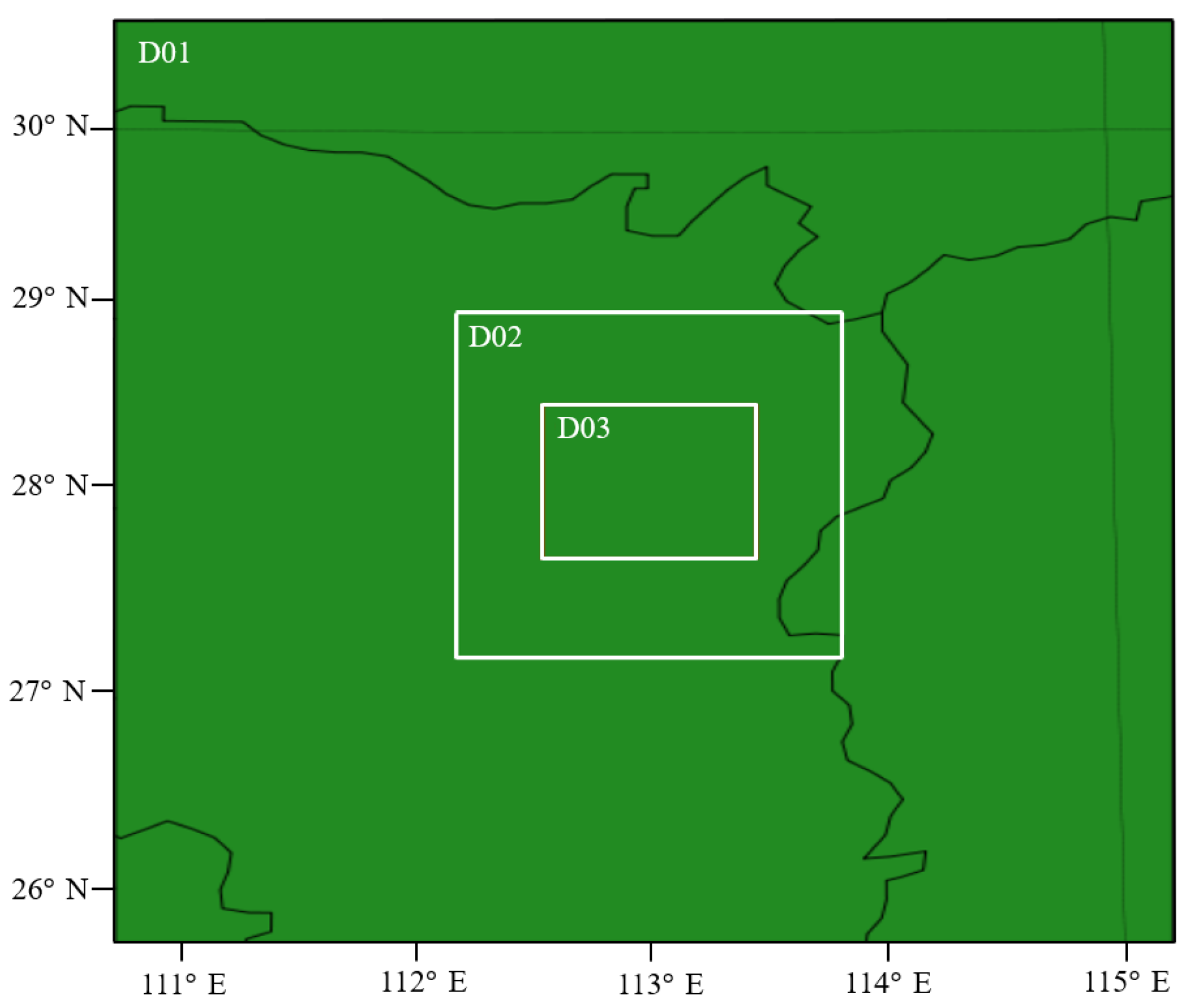
It is generally acknowledged that the parameterization schemes of the WRF model possess a vital significance to the simulation performance. Subsequently, sensitivity analyses for parameterization schemes were conducted via WRF-BEP simulations to accurately investigate the urban wind flow characteristics. The wind speed and direction extracted from the WRF-BEP simulations were compared with the field-measurement data from the National Weather Science Data Center, China.

2.1. Model Setup

The meso-scale WRF-BEP model was selected to simulate the wind flow from 19 March 2022 00:00:00 to 23:59:59. As shown in Figure 1, the WRF-BEP model adopts three nested domains with a spatial coverage of 450 km × 544.5 km for D01 (100 × 121 grid points with a horizontal resolution of 4.5 km), 163.5 km × 204 km for D02 (109 × 136 grid points with a horizontal resolution of 1.5 km) and 90.5 km × 90.5 km for D03 (181 × 181 grid points with a horizontal resolution of 0.5 km). The adjacent domains utilize a two-way coupling strategy for information transmission, and the center of the outermost domain (the study urban region) is located at 28.16° N, 112.98° E. A total of 45 vertical levels are utilized in the WRF-BEP model, with the first level of 10 m from the ground.
Considering the PBL parameterization scheme significantly influences the numerical performance of the WRF-BEP model, three PBL schemes were configured in the model setups, namely Yonsei University (YSU), Mellor-Yamada-Janjic (MYJ) and Bougeault–Lacarrere (BouLac). Other physical parameterization schemes are displayed in Table 1. Specifically, the land surface (LS), microphysics (MPH), surface layer (SL), cumulus (CU) and radiation (RA) are set as the Noah multi-physics (MP), single-moment 6-class (WSM6), revised MM5, Grell 3D and RRTMG, respectively.

2.2. Sensitivity Study of WRF-BEP Simulation

2.2.1. Evaluation Metric

Three commonly used statistical metrics were selected to evaluate the accuracy of WRF-BEP simulations, namely the mean absolute error (MAE), mean absolute percentage error (MAPE) and root-mean-square error (RMSE). Their calculation formulas are given as follows:
M A E = 1 N i = 1 N | v i v i ^ |
M A P E = 1 N i = 1 N | v i v i ^ v i |
R M S E = 1 N i = 1 N ( v i v i ^ ) 2
where N is the total number of sampling points while v i and v i ^ are the WRF simulated and observed wind speeds, respectively.

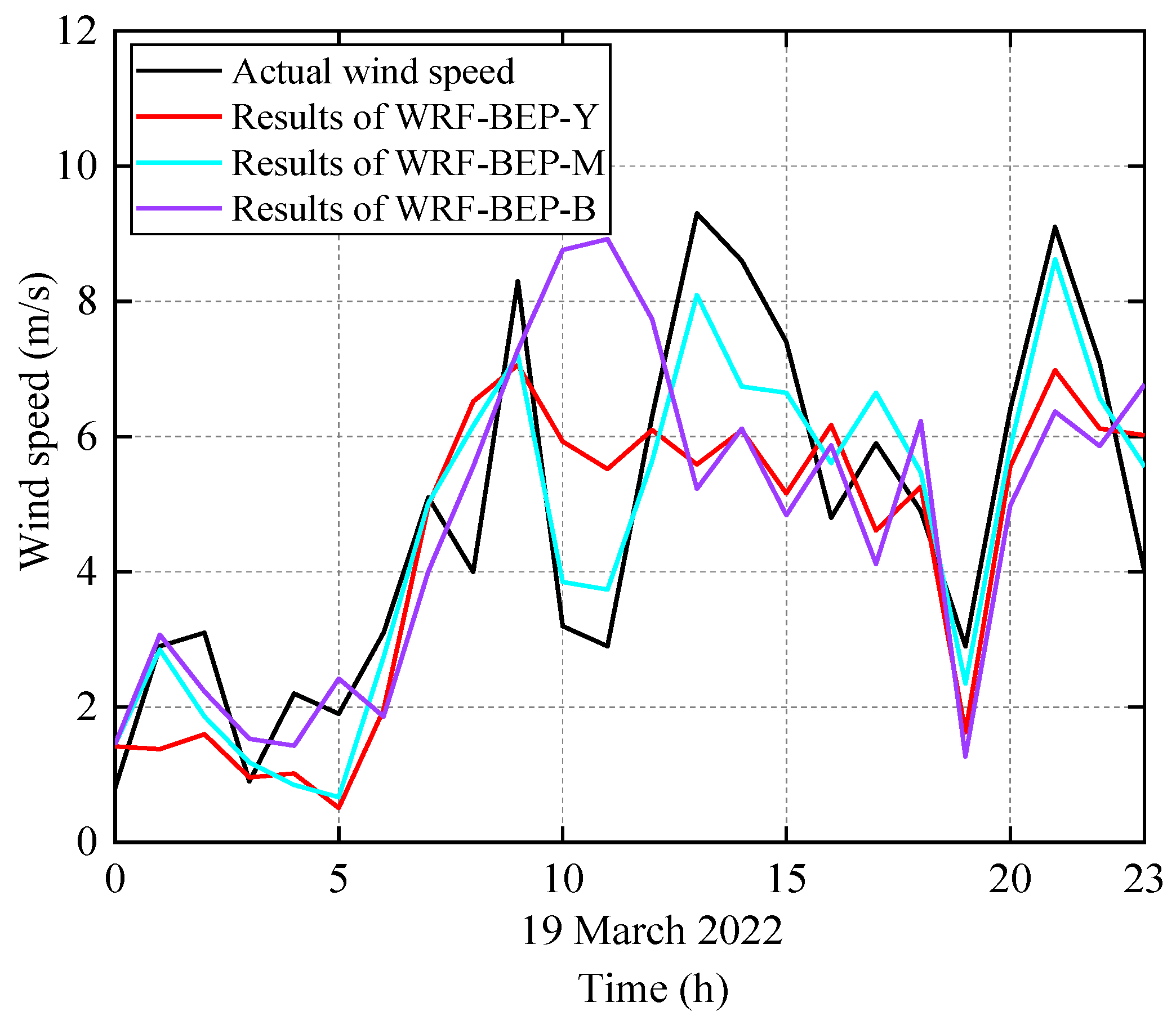
2.2.2. Results Analysis

The WRF-BEP simulation results were compared with the field-measurement (actual) wind speeds of the 10 m height from the National Weather Science Data Center, China, as depicted in Figure 2 (with a sampling interval of one hour). The evaluation metrics were accordingly calculated and are presented in Table 2. The wind speed time history in Figure 2 indicates that the simulated results of the WRF-BEP-M model best capture the trend of the observations. Additionally, the lowest values of RMSE, MAE and MAPE in Table 2 associated with the WRF-BEP-M scheme suggest it possessed the highest wind speed simulation accuracy. Therefore, the WRF-BEP-M scheme was used in all urban wind flow simulations of the current case study.

3. Micro-Scale CFD Simulation and Validation

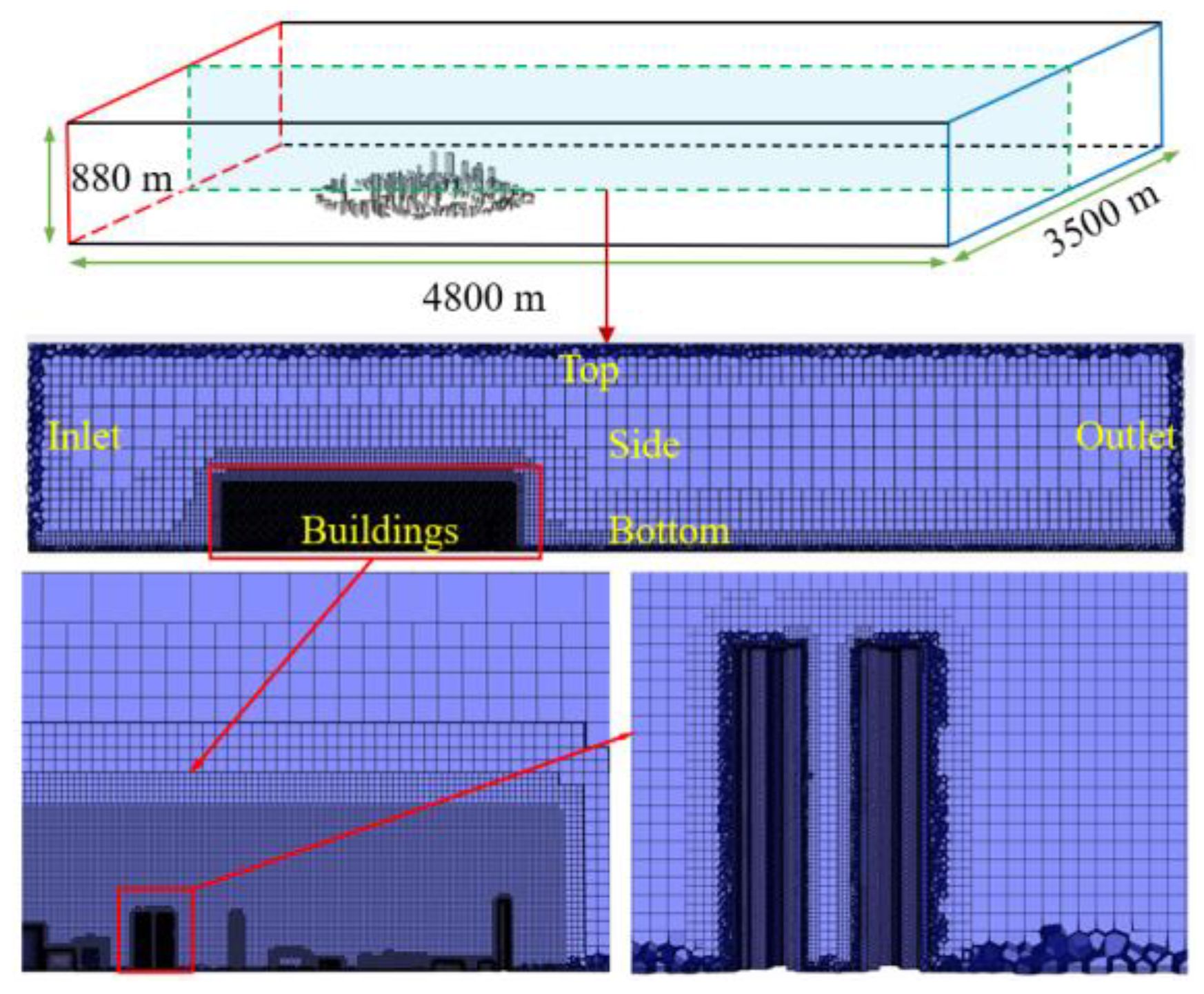
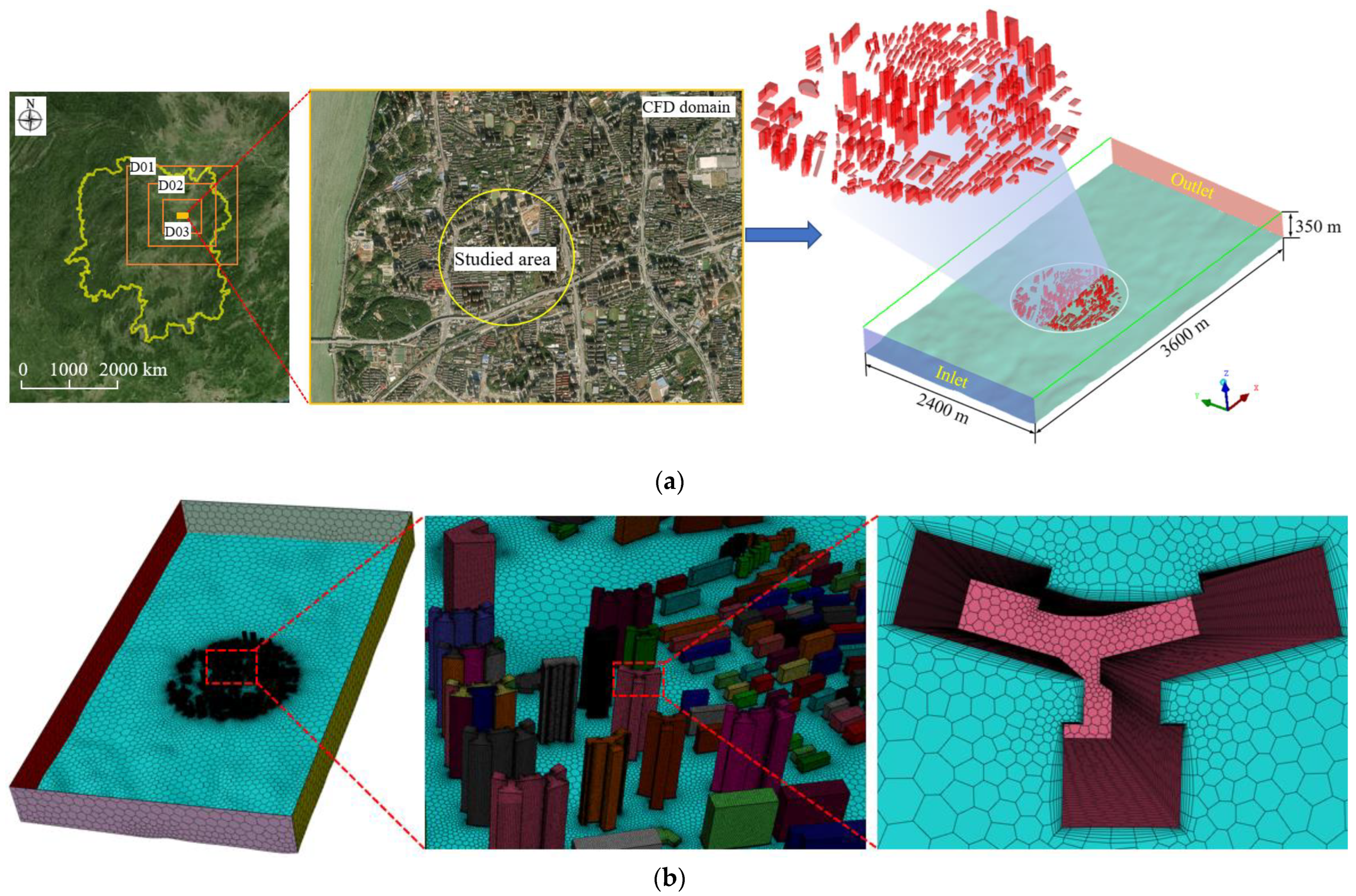
3.1. Computational Domain and Boundary Condition

A three-dimensional (3D) computational domain embedded with all actual building structures in the study area was established for the micro-scale CFD simulations, as shown in Figure 3. The polyhedral-hexahedral core grids are generated using Ansys Fluent Meshing, and the total cells of the computational domain is about 7.6 million. To better capture the flow field characteristics around the buildings, five mesh layers were utilized near the structural surface, with the grid size ranging from 0.7 m to 2 m. The largest grid size (far away from the buildings) was set to be 50 m, and the far-field boundary conditions are depicted in Table 3. Specifically, the variables of the inlet boundary condition, including the inlet wind velocity magnitude ( v ), turbulent kinetic energy ( k ) and specific dissipation rate ( ω ), are set based on the formulas below [21,22]:
v ( z ) = u * κ l n ( z + z 0 z 0 )
k ( z ) = u * 2 [ C u 1 l n ( z + z 0 z 0 ) + C u 2 ] 2
ω ( z ) = u * κ ( z + z 0 ) [ C u 1 l n ( z + z 0 z 0 ) + C u 2 ] 2
where z denotes the height above the ground; u * is the friction velocity; κ is the von Karman constant; z 0 is the roughness length; C u 1 and C u 2 represent turbulence boundary parameters.

3.2. Validation of Numerical Algorithm

To validate the simulation accuracy of the micro-scale CFD numerical algorithm, wind tunnel tests were conducted to obtain the wind speed and TI at selected locations. The experiment was performed in the wind tunnel at Changsha University of Science and Technology. The building models of all actual structures in the study urban region possessed a scale of 1:250, as shown in Figure 4a. A total of 144 monitoring points were selected to obtain the wind speed by the Irwin sensor and electronic pressure scanning module (PSI DTC Initium with an accuracy of 0.06% and sampling frequency of 350 Hz), and 64 of them were arranged in the core area as displayed in Figure 4b. It is noted that the circles in Figure 4b share the same center of the wind tunnel turntable.

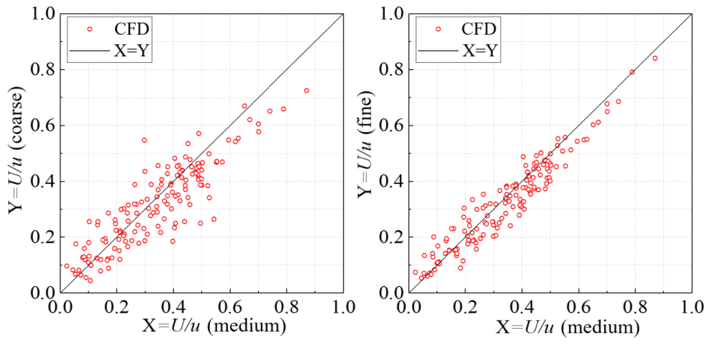
3.2.1. Grid Independence Study

In this grid independence study, the inlet velocity was set as 8 m/s, and the static pressure of the outlet was zero. The velocity-pressure coupling was accomplished based on the SIMPLEC algorithm, and the second-order discretization was applied to the momentum and turbulence transport equations. The shear stress transfer (SST) k-ω model is utilized to solve the closure problem of turbulence, and the governing equations are provided below [23,24]:
t ( ρ k ) + x j ( ρ k u j ) = x j ( Γ k k x j ) + G ¯ k Y k
t ( ρ ω ) + x j ( ρ ω u j ) = x j ( Γ ω ω x j ) + G ω Y ω
where u is the CFD simulated wind velocity; x i and x j denote the spatial coordinates; t is the time; ρ symbolizes the air density; Γ , Γ k and Γ ω represent the effective diffusion coefficients of u , k and ω , respectively; G ¯ k and G ω indicate the generations of k and ω , respectively; Y k and Y ω remain the dissipations of k and ω , respectively. The wind velocity (U) measured at 144 monitoring points in the wind tunnel was used to calculate the target indicator (U/ u ) for the grid-independent test. Specifically, the cell numbers of the three tested grid sets are 3.8 million, 7.6 million and 11 million (corresponding to coarse, medium and fine meshes), respectively. The simulation results with various grid numbers are compared in Figure 5. It can be concluded from Figure 5 that the target indicators obtained from the medium mesh are close to those from the fine mesh. On the other hand, the difference in the target indicators between the coarse and medium meshes remains large. Therefore, the medium mesh (7.6 million) was selected for all the CFD simulations of the current case study. It should be noted that the residual curves in all simulations converged below the value of 10−4.

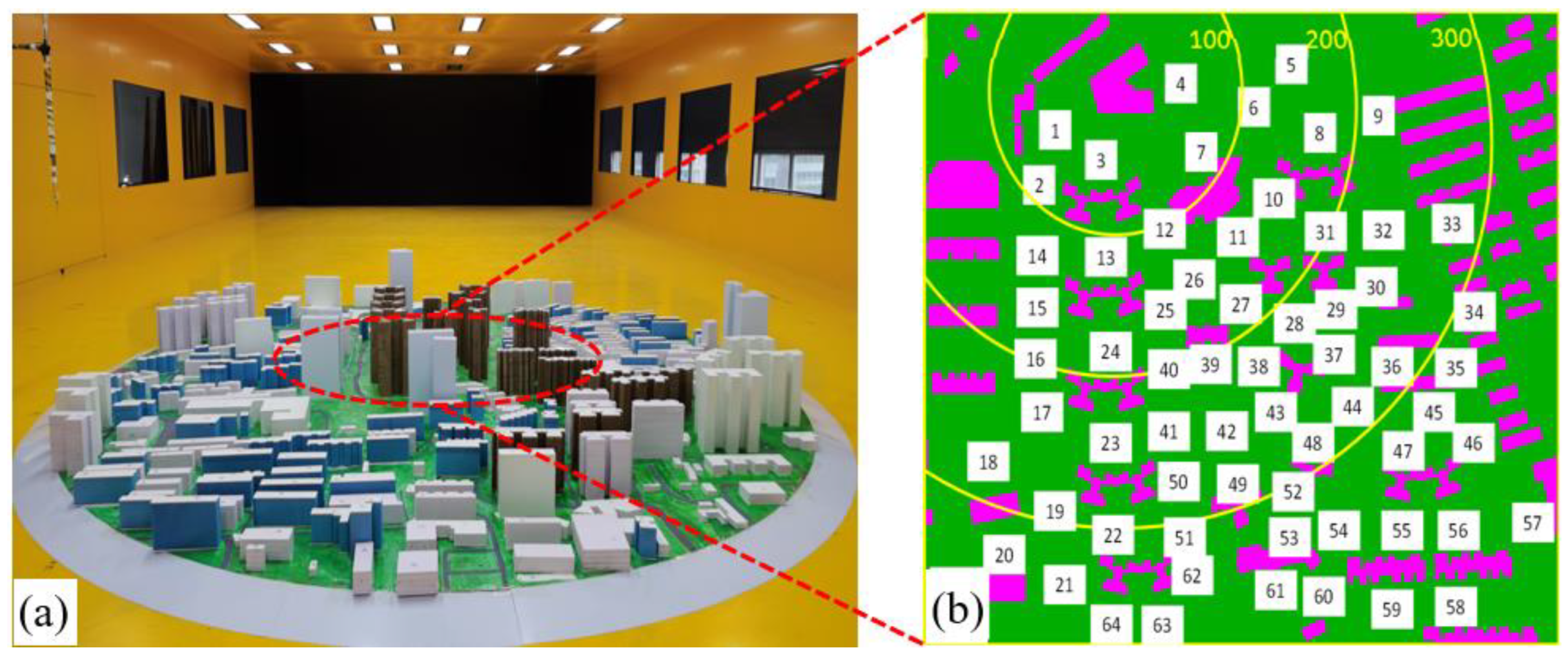
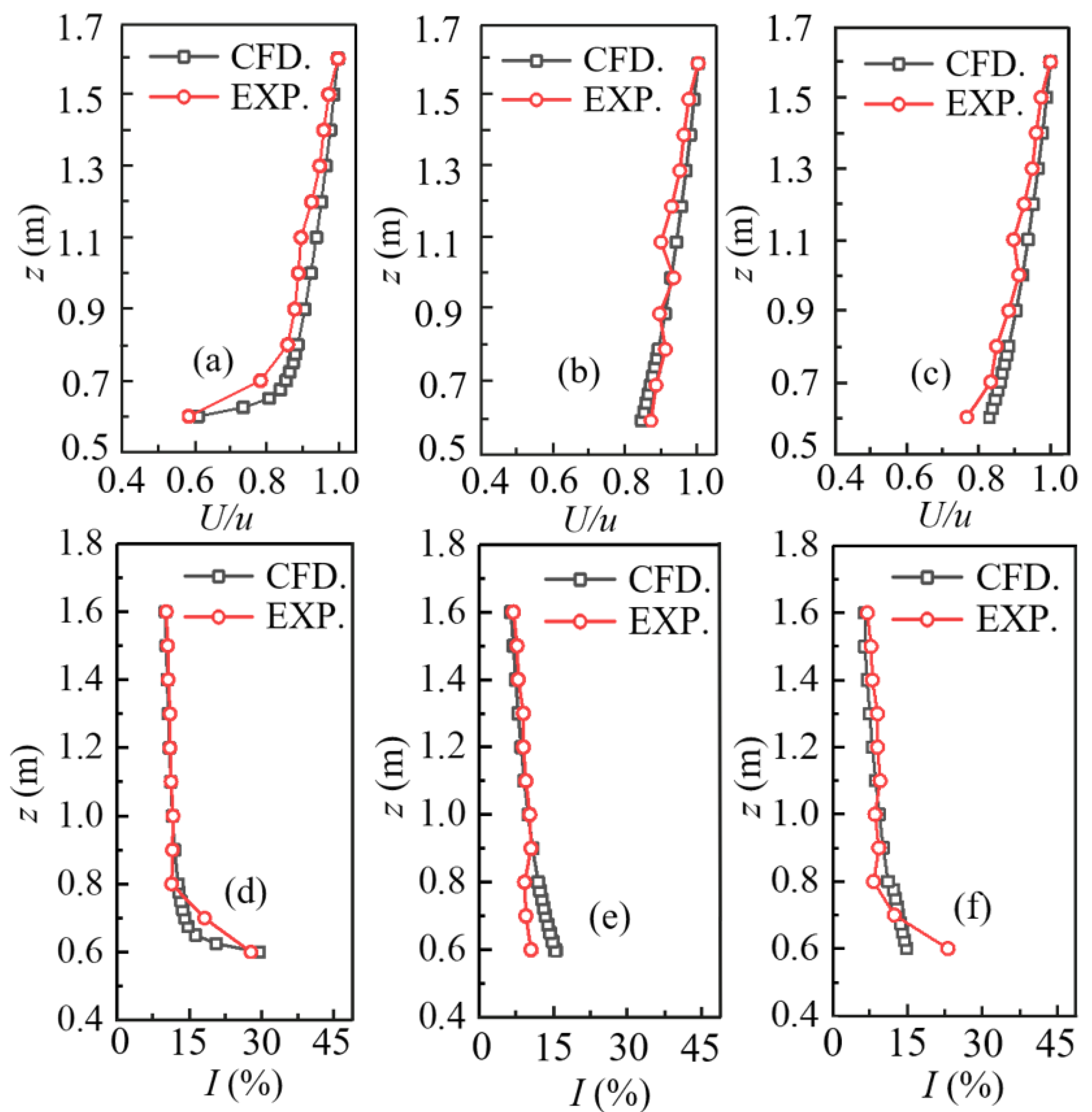
3.2.2. Validation Using Wind Tunnel Test

The micro-scale CFD simulations with the SST k-ω turbulence model were validated by comparing the numerically obtained wind speeds and TIs at monitoring points 4, 5 and 6 with those measured in the wind tunnel using the cobra probe (Turbulent Flow Instrumentation Australia with an accuracy of ±0.5 m/s and sampling frequency of 500 Hz). Figure 6 shows the comparison results of the wind speed ratio (U/u) and TI at various heights above the ground. The results in Figure 6 present a high agreement between the CFD simulations and wind tunnel measurements with a minimum deviation of 0.2%, maximum deviation of 8.1% and mean deviation of 4.9%, suggesting the micro-scale CFD numerical algorithm used in this case study was reliable with good simulation accuracy. It is noted that the U/u and TI profiles below 0.6 m are not depicted in Figure 6 due to the poor measurements of experimental data near the floor surface.

4. Wind Resource Assessments with Coupled WRF-BEP-RANS Simulation

4.1. Wind Resource Assessment Metric

The WPD and TI are two widely used metrics for effective WRAs. As an indicator for evaluating the available wind power for a certain period, the WPD is calculated as [18]:
W P D = 1 2 ρ u 3
The classification of WPD and relevant descriptions are depicted in Table 4 [18]. For the TI in the micro-scale CFD simulations, a convenient calculation is expressed as [18]:
I = 2 k 3 u
To ensure the wind turbine safety and power output, the TI of 18% is set as the maximum acceptable limit for selecting the potential installation locations of micro-wind turbines in the case study [18,25]. Obviously, the best installation location would target maximum WPD and minimum TI.

4.2. Wind Resource Assessment Procedure

The procedure of the proposed multi-scale wind resource assessments was composed of three main steps. A detailed description of each step is presented as follows.
Step 1: data collection. The local meteorological data and the building and terrain data were prepared for accurate evaluations of the urban wind resource. Specifically, the statistical wind data (including both speed and direction) for a long period (e.g., 10 years) was acquired to determine the dominant wind speed and direction of a specific site. According to the obtained building and terrain data, the numerical model can be established for coupled multi-scale simulations of urban wind flow.
Step 2: numerical wind resource estimation. The inlet conditions of the RANS simulations were first extracted from the WRF-BEP model on the basis of the dominant wind speed and direction from Step 1. Then, the numerical wind energy assessments were conducted based on the obtained values of WPD and TI. Specifically, the studied area possesses no potential for wind energy development if the WPD value is lower than 100 W/m2 or the TI value is higher than 18%. For locations with TI lower than 18%, the wind energy potential is further determined according to Table 4.
Step 3: installation arrangements of micro-wind turbines. Appropriate installation locations and the lowest installation heights for micro-wind turbines in the urban areas were determined based on the principles from Step 2.

5. Case Study

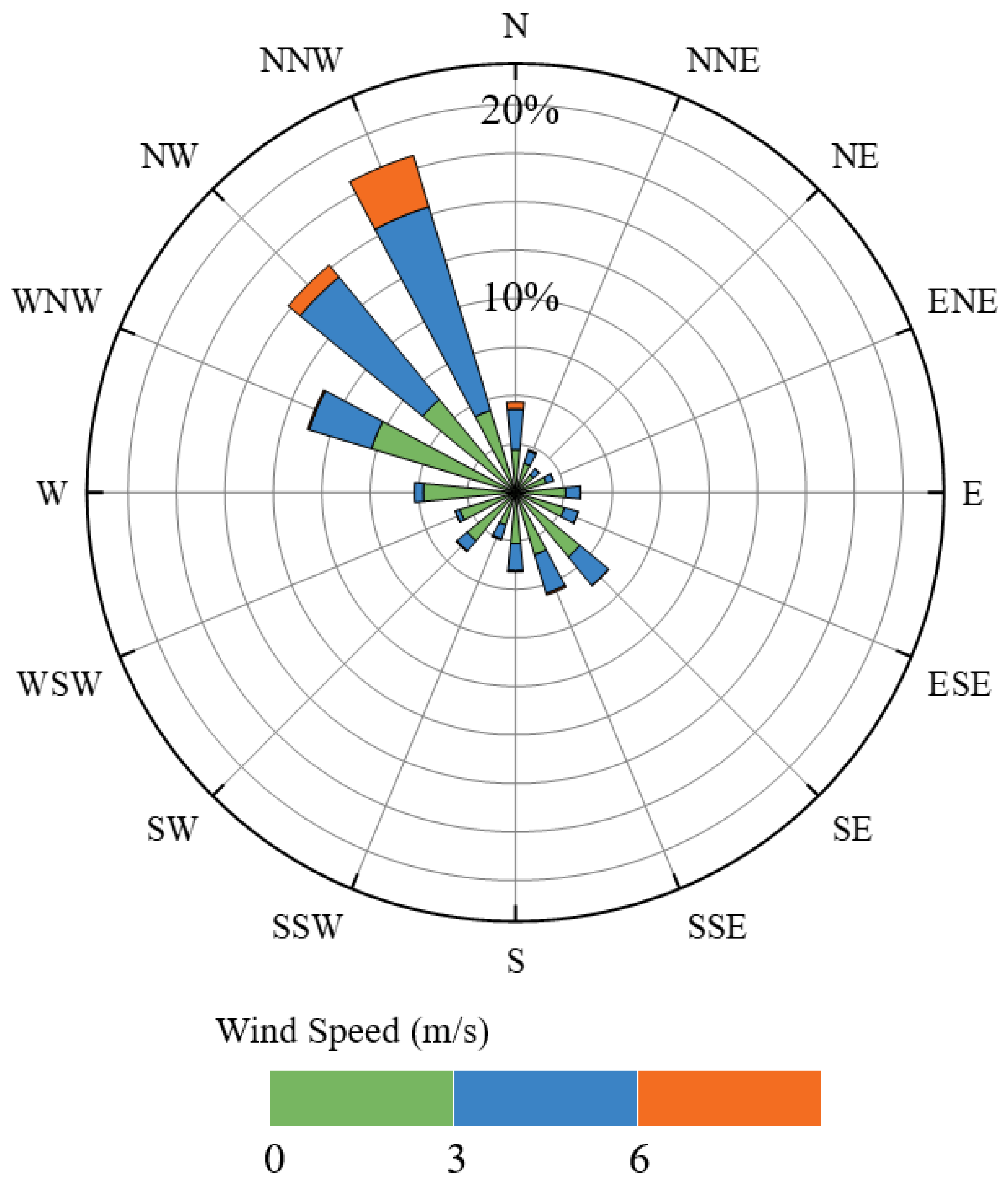
5.1. Local Meteorological Data and Numerical Setting

To obtain reliable results for wind resource assessments, 11 years of statistical wind data (including both speed and direction) from 2010 to 2021 at Changsha meteorological station was used. The yearly-period wind rose consisting of 16 sectors is presented in Figure 7. As suggested by Figure 7, the dominant wind direction of the study region is from the north-north-west (NNW) to the south-south-east (SSE) with an average speed of 2.51 m/s. The WRAs in the current case study were focused on such a wind condition.
A 3D numerical model for the WRAs of the study area with a diameter of 1.2 km was accordingly established (including detailed terrain conditions and realistic architectural structures), as shown in Figure 8a. Specifically, the complex terrain obtained from the Blender software was merged with buildings through the Ansys ICEM software. Then, the “dirty” model was imported into Ansys Fluent Meshing with the Fault-Tolerant Meshing Workflow to generate the polyhedral-hexahedral core grids, as displayed in Figure 8b. While the velocity-inlet boundary condition of the micro-scale CFD simulations was extracted from the meso-scale WRF-BEP model with the MYJ PBL scheme, other boundary conditions along with the grid setting and numerical algorithm were consistent with those validated in Section 3.

5.2. Wind Power Potential

Among all viable mounting schemes for wind turbines on or around high-rise buildings in a highly-urbanized area [3,17], the micro-wind turbine integration into building skin and installation on the building roof was selected for further analysis of the wind power potential in the target area.

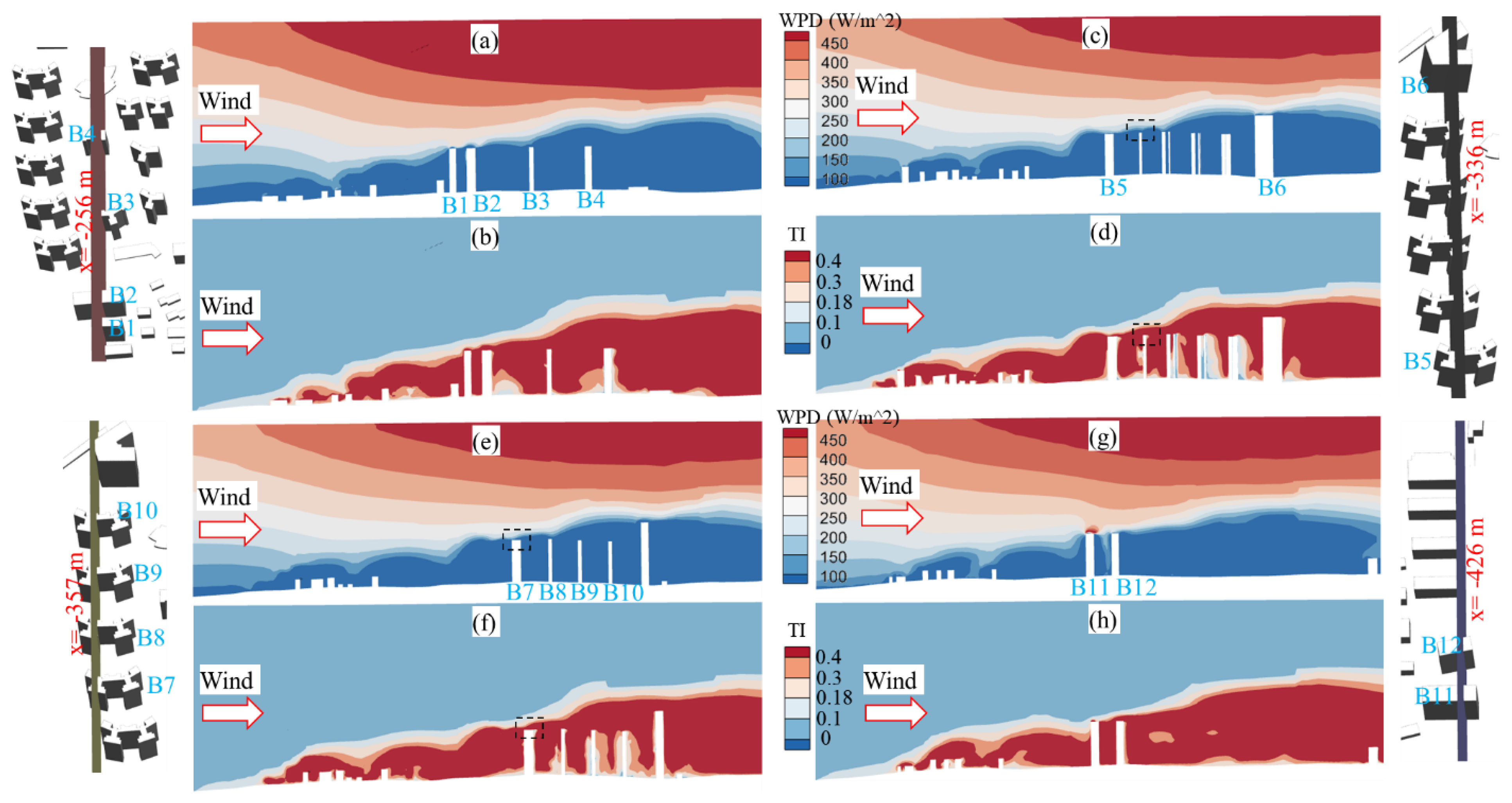
5.2.1. Wind Turbines Integrated into Building Skin

For the assessment of the wind power potential of wind turbines integrated into the building skin, it was important to characterize the flow features (in terms of WPD and TI) along the building height. Figure 9 depicts the simulated WPD and TI contours at z = 50 m, 100 m, 120 m and 140 m in the x-y plane for the study area, where z represents the height from the ground. Considering that most of the buildings are in an area with low WPDs (less than 100 W/m2) and high TIs (higher than 18%), it can be concluded that the integration of micro-wind turbines into the building skin is not recommended in this highly-urbanized region. The major reason may result from the shadow effects of front high-rise buildings. Specifically, a significant portion of the rear buildings were located in the wake flow region of the front buildings with low WPDs and high TIs.

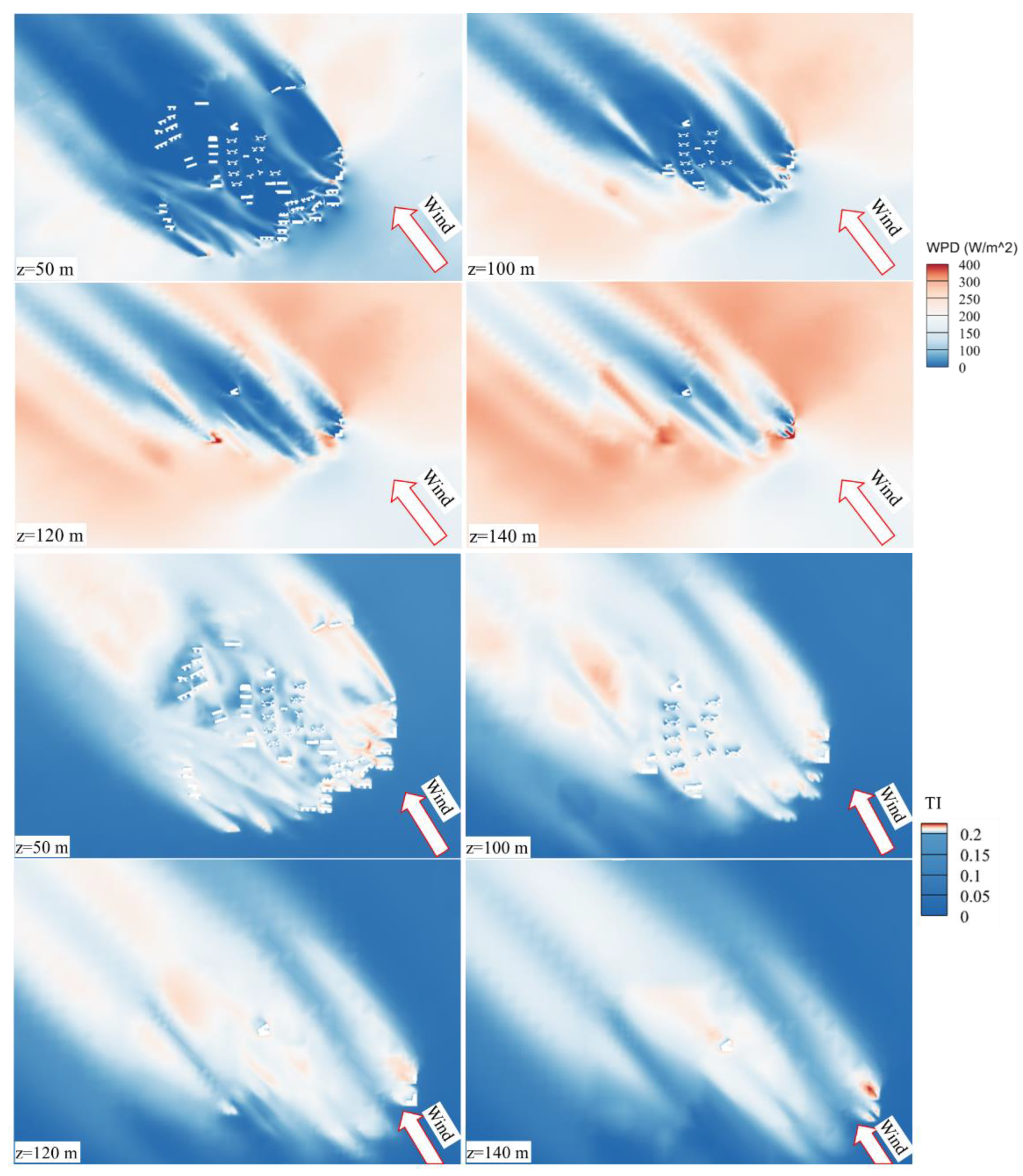
5.2.2. Wind Turbines Installed on Building Roof

For the assessment of the wind power potential of wind turbines installed on the building roof, it was important to characterize the flow features (in terms of WPD and TI) over the building top. Figure 10 depicts the simulated WPD and TI contours at x = −256 m, −336 m, −357 m and −426 m in the y-z plane, where the xyz coordinate origin is located at the center of the study area. It is noted that these locations are intentionally selected to include a good number of high-rise buildings, and these target buildings for WRAs are marked as B1–B12 in Figure 10. According to Figure 10a,b, the buildings B1–B4 generally possess an excellent developing capacity for wind energy, with WPDs around their roofs ranging from 200 W/m2 to 300 W/m2 and the corresponding TIs at a reasonable height above the roofs smaller than 18%. Compared to buildings B3 and B4, buildings B1 and B2 required relatively lower heights above the roof to limit the TI to the maximum allowable value for micro-wind turbine installation. Figure 10c,d suggest that buildings B5 and B6 also had outstanding wind power potential, with WPDs around their roofs exceeding 200 W/m2 and the corresponding TIs at a reasonable height above the roofs smaller than 18%. Compared to building B6, building B5 required a relatively lower height above the roof to limit the TI to the maximum allowable value for micro-wind turbine installation. Similar observations from Figure 10e–h suggest that buildings B7–B12 can also be utilized for rooftop wind energy harvesting due to their high WPDs and low TIs at a reasonable height above the roofs. Among them, buildings B7 and B11 require a relatively lower height above the roof to limit the TI to the maximum allowable value for micro-wind turbine installation.
Although it is widely recognized that the installation of micro-wind turbines on building roofs should generally avoid the separation bubble (associated with low WPDs and high TIs due to the complex flow characteristics), a close examination of the simulated WPDs and TIs along the x and y axes can facilitate accurate determination of the installation locations on each building roof. For example, Figure 10c–f present WPDs and TIs around the roof of building B7 (highlighted by the black dashed frame) at two different locations (with x = −336 m and −357 m, respectively). As shown in the figures, similar WPDs are observed for these two locations, while a lower height above the roof is required to limit the TI to the maximum allowable value for the location of x = −357 m compared with that for the location of x = −336 m. The major reason is that the front building B5 presented less aerodynamic interference effects on building B7 at the location of x = −357 m than at the location of x = −336 m. Hence, the location of x = −357 m on the roof of building B7 was more suitable for micro-wind turbine installation.
In addition to a close examination of the simulated WPDs and TIs along the x and y axes, their profiles along the height above the roof (Z) could also be utilized to refine the installation locations of micro-wind turbines. For buildings B1, B2, B5, B7 and B11 with a great roof wind power potential based on the above-mentioned discussion, the simulated WPD and TI profiles along Z for various roof locations are presented in Figure 11. For the selected four roof locations of building B1, Figure 11a suggests that the lowest wind turbine installation height for locations B1-1, B1-2 and B1-3 was approximately 8 m above the roof (with TIs smaller than 18%), and their WPDs were around 260 W/m2, 270 W/m2, 220 W/m2, respectively. On the other hand, the lowest wind turbine installation height for location B1–4 was approximately 13 m (with TIs smaller than 18%), and its WPD was slightly higher than 200 W/m2. For the selected locations of buildings B2, B5 and B7, Figure 11b–d indicate that the lowest turbine installation height for locations B5-1, B5-2, B5-3 and B5-4 was beyond 15 m (with the corresponding WPD around 200 W/m2) while this value for all other locations increased to around 20 m (with the corresponding WPD in the range between 150 W/m2 and 300 W/m2). For the selected five locations of building B11, Figure 11e shows the lowest turbine installation heights for locations B11-2 and B11-3 were around 5 m and 7 m, respectively (with the corresponding WPDS around 300 W/m2 and 400 W/m2, respectively). On the other hand, the lowest turbine installation heights for locations B11-1, B11-4 and B11-5 ranged from 10 m to 15 m (with a similar WPD value of about 300 W/m2). Accordingly, B1-1, B1-2, B1-3, B11-2 and B11-3 were the optimal roof wind turbine installation locations in this case study.

5.3. Discussion

For the five optimal wind turbine installation locations B1-1, B1-2, B1-3, B11-2 and B11-3 at building roofs, further numerical investigation was conducted to examine the influence of the terrain conditions, PBL parameterization schemes and turbulence models on WRAs based on the coupled meso-scale WRF-BEP and micro-scale CFD simulations.

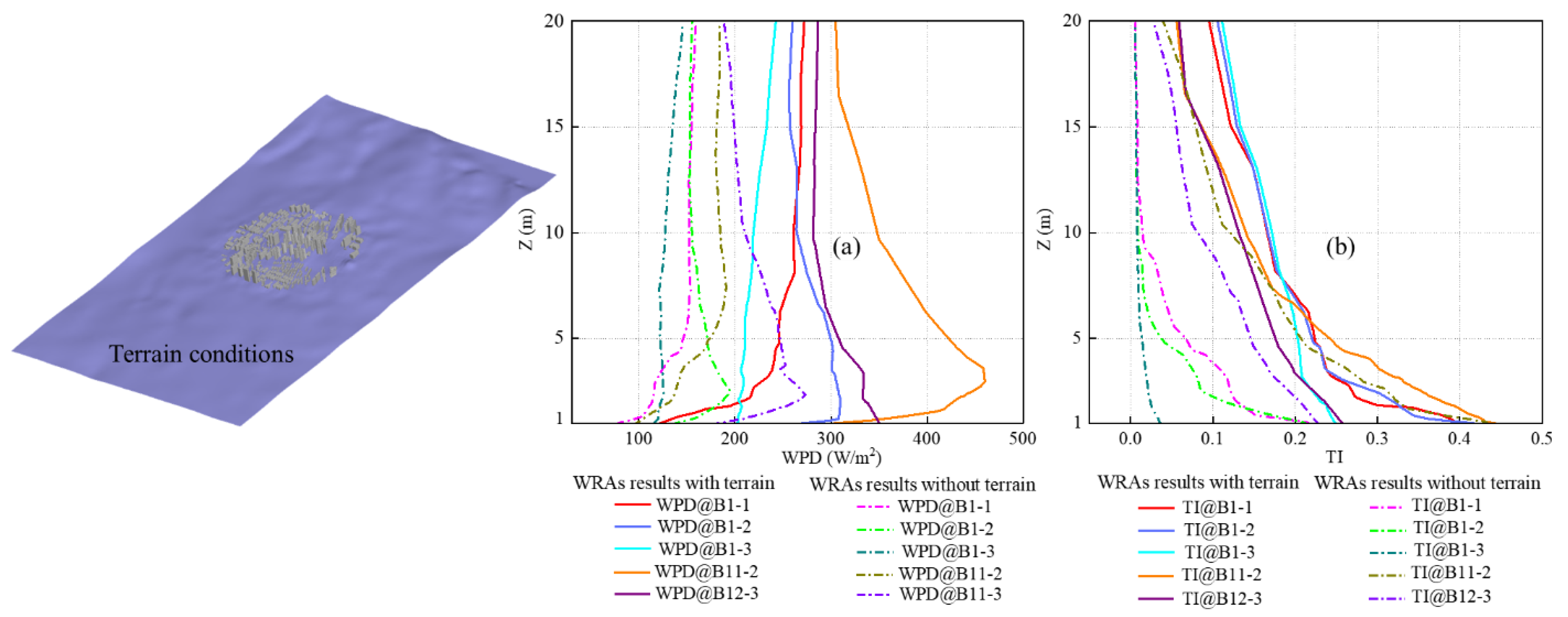
5.3.1. Terrain Condition

The simulated WPD and TI profiles with and without the considerations of terrain conditions are depicted in Figure 12. From Figure 12, it is obvious that both WPD and TI were underestimated for all five locations in the case that the terrain conditions are not considered in the multi-scale numerical simulations. For example, the WPD and TI values of B1-1 (at 8-m height from the roof) were 260 W/m2 and 17%, respectively, in the simulation with the terrain. However, they were reduced to 150 W/m2 and 3% in the simulation without the terrain. This observation suggests that the significant influence of the terrain conditions on the multi-scale numerical assessment of urban wind resource cannot be ignored.

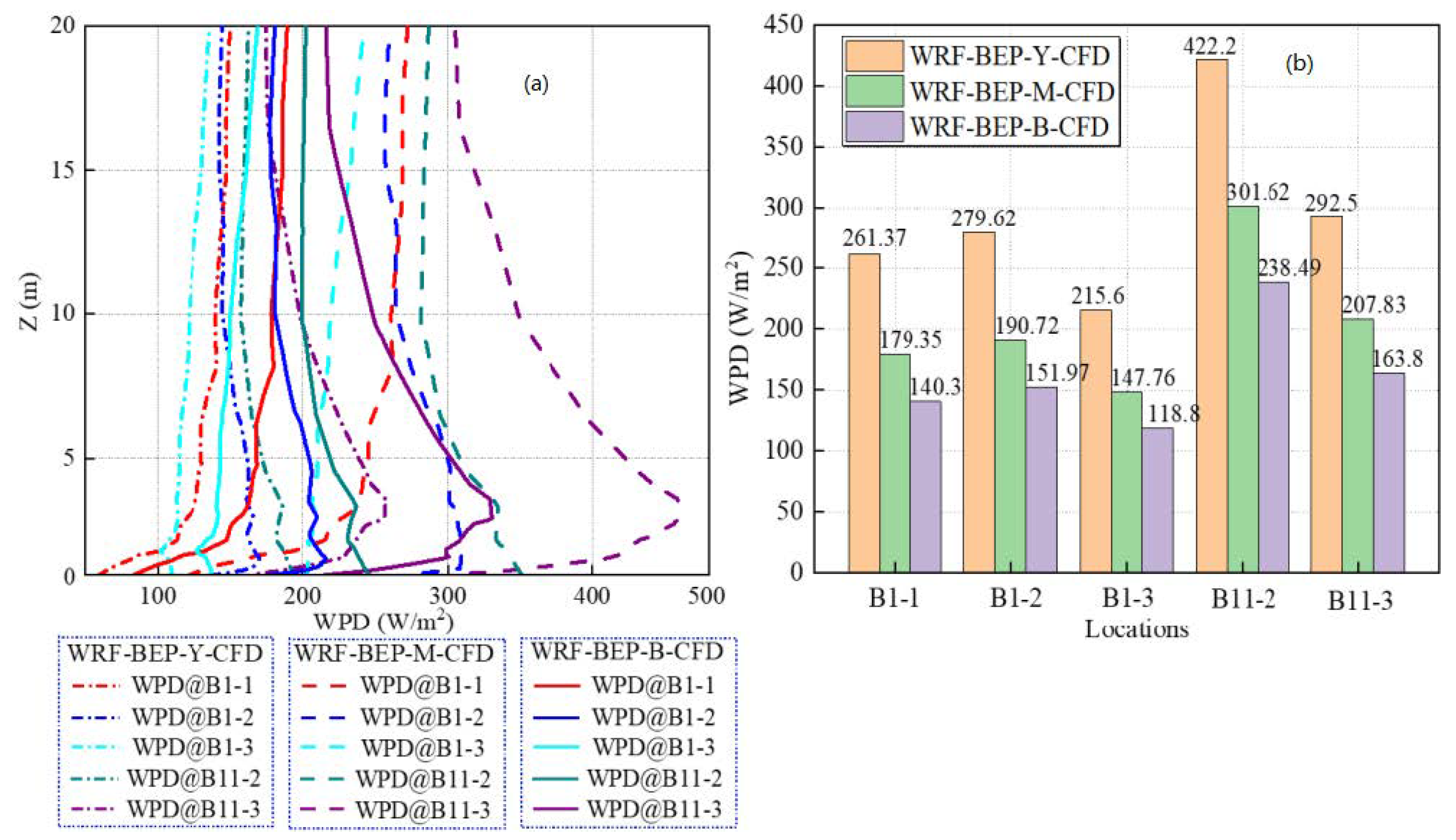
5.3.2. PBL Parameterization Scheme

The simulated WPD profiles based on three different PBL parameterization schemes in the WRF-BEP model are shown in Figure 13a. Compared to the simulated WPDs of WRF-BEP-M-CFD, those resulting from both WRF-BEP-B-CFD and WRF-BEP-Y-CFD decreased for all five optimal installation locations. Furthermore, the simulated WPDs using these PBL parameterization schemes for the five optimal locations at the lowest installation heights are depicted in Figure 13b. As shown in the figure, it can be clearly found that both WRF-BEP-B-CFD and WRF-BEP-Y-CFD cases significantly underestimated the simulated WPDs compared to those from WRF-BEP-M-CFD. For example, the simulated WPD of WRF-BEP-M-CFD for location B1-1 was 260 W/m2 and was 80 W/m2 and 120 W/m2 higher than those of WRF-BEP-B-CFD and WRF-BEP-Y-CFD, respectively. This observation suggests that the WPDs are very sensitive to the used PBL parameterization schemes. It is noted that the TI results are not discussed here because the WRF-BEP-Y scheme cannot provide the turbulent kinetic energy.

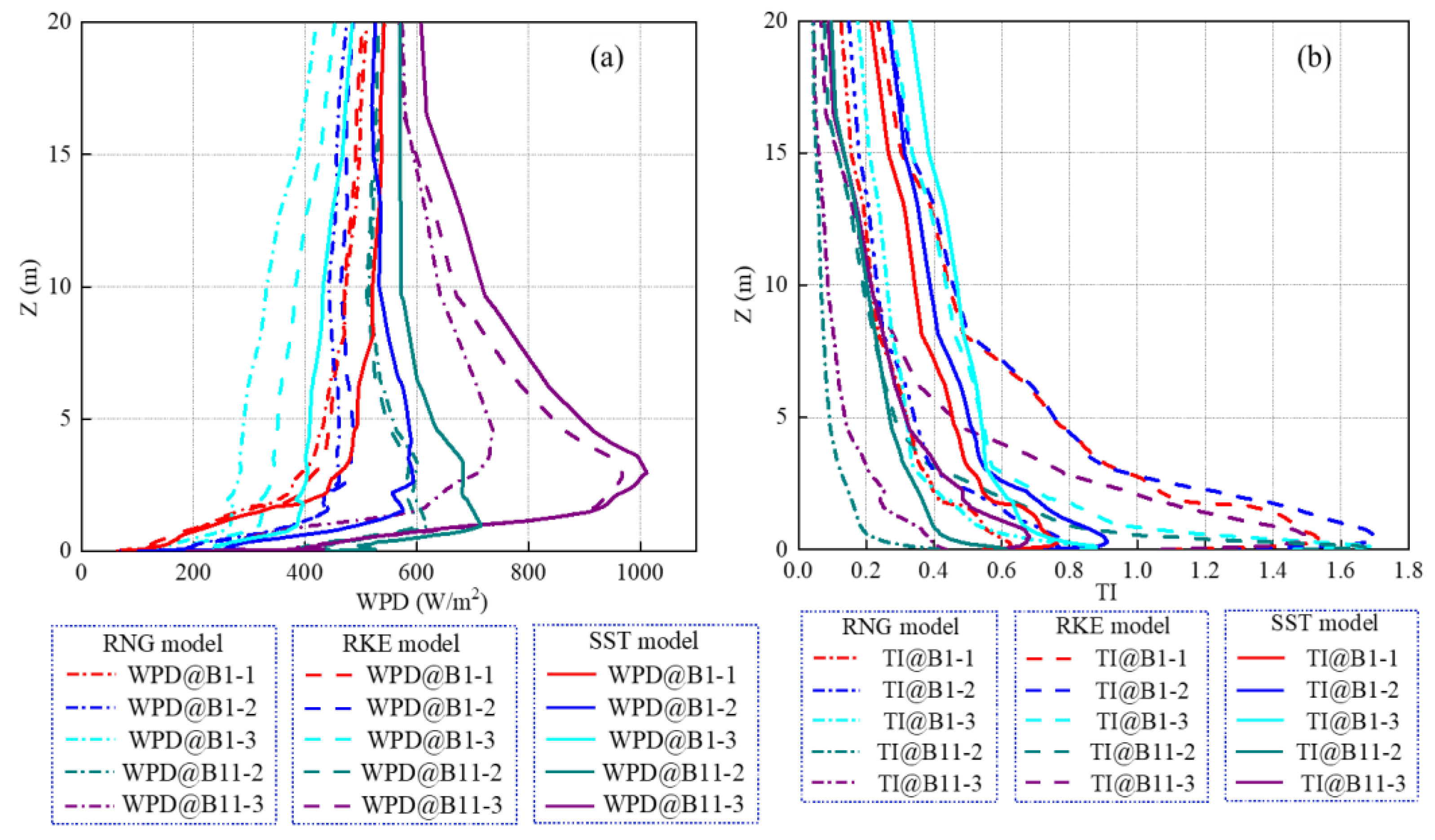
5.3.3. Turbulence Modeling

Three widely used turbulence models for urban wind simulations are discussed here to investigate their effects on WRAs, namely the realizable k-ε (RKE) [26], re-normalization group (RNG) k-ε [27] and SST k-ω [28] models. The simulated profiles of WPD and TI are presented in Figure 14. From Figure 14, it can be concluded that the SST and RKE models generally generated similar WPD and TI values, and they were significantly larger than those from the RNG model. For example, the simulated WPDs (and TIs) based on the SST, RKE and RNG models at 8-m height above the B1-3 roof were around 420 W/m2 (with TI of 49%), 380 W/m2 (with TI of 47%) and 310 W/m2 (with TI of 27%), respectively. Hence, it is important to systematically validate the used turbulence model under realistic meso-scale urban flow conditions (as the inlet velocity conditions of micro-scale CFD simulations).

6. Concluding Remarks

This case study presented a multi-scale numerical methodology coupling the WRF-BEP model and RANS equations to conduct WRAs in a highly-urbanized area (with realistic terrain conditions), namely the Generic Times International Community in Changsha, China. The wind simulations from the meso-scale NWP and micro-scale CFD models were validated by the on-site monitoring data and wind tunnel test data, respectively. A close examination of the coupled WRF-BEP and RANS simulation results was performed to identify the optimal locations (with high WPDs and low TIs) for the installation of micro-wind turbines on buildings. The significant impacts of terrain conditions, PBL parameterization schemes and turbulence models on WRAs were highlighted. The main conclusions are summarized as follows.
  • Both WPD and TI were underestimated in the case that the terrain conditions were not considered, and the significant influence of the terrain conditions on the multi-scale numerical assessment of urban wind resource cannot be ignored.
  • Compared to the simulated urban flow from PBL parameterization schemes of YSU and BouLac, the results from the MYJ scheme presented the minimum difference with the field-measured wind speeds from the National Weather Science Data Center, China. Specifically, the obtained values of RMSE, MAE and MAPE were 0.98, 0.83 and 24.18%, respectively. The WRF-BEP-RANS simulations with both the YSU and BouLac schemes underestimated the WPDs compared to those of the MYJ scheme.
  • The mean wind and TI profiles in RANS simulations with the SST k-ω turbulence model showed fairly good agreement with wind tunnel measurements. Compared to the SST turbulence model simulations, the RKE turbulence model generated similar WPDs and Tis, while the RNG turbulence model significantly underestimated these results.
  • Considering the intense negative aerodynamic interference among buildings of the highly-urbanized area in this case study, the integration of micro-wind turbines into building skin was not recommended. For the building roof, five optimal installation locations were identified by systematically examining the simulated WPDs and TIs.
Although the proposed multi-scale simulation methodology coupling the WRF-BEP model and RANS equations presented great promise for urban WRAs, research efforts are needed to significantly reduce the high computational demand (e.g., about one week for each WRF-BEP simulation and two days for each CFD simulation of current case study on the computer of Intel Xeon Gold 6226R CPU @ 2.9 GHz and 2.89 GHz) and perform uncertainty quantifications in the numerical assessments of the urban wind resource.

Author Contributions

L.M.: Conceptualization, data curation, formal analysis, funding acquisition, methodology, software, validation, writing—original draft, Writing—review and editing. Y.H.: Funding acquisition, methodology, project administration, resources, supervision, writing—review and editing. L.S.: Conceptualization, supervision, validation, writing—review and editing. C.C.: Funding acquisition, resources, supervision, writing—review and editing. T.W.: Methodology, resources, supervision, writing—review and editing. All authors have read and agreed to the published version of the manuscript.

Funding

This work was supported by the National Natural Science Foundation of China (Grant No. 51822803, 52178452, 51808059, 52108433), the Science and Technology Innovation Talent Project of Hunan Province (Grant No. 2021RC4031), the Science Fund for Creative Research Groups of Hunan Province (Grant No. 2020JJ1006), the Natural Science Foundation of Hunan Province (Grant No. 2021JJ40587), the Innovation-Driven Project of Central South University (No. 2020CX009) and the Postgraduate Research Innovation Project of Changsha University of Science and Technology (Grant No. CXCLY2022029).

Data Availability Statement

The data of wind speeds of the 10 m height are from the National Weather Science Data Center, China, which can be found here: data.cma.cn/. The rest data presented in this study are available on request from the corresponding author.

Conflicts of Interest

The authors declare that they have no conflict of interest or personal relationships that could affect the work reported in this paper.

Nomenclature

BEPbuilding effect parameterization C u 1 ,   C u 2 turbulence boundary parameters
BouLacBougeault-Lacarrere G ¯ k ,   G ω generation of k ,   ω
CFDcomputational fluid dynamics k turbulent kinetic energy
CUcumulus t time
LiDARlight detection and ranging u CFD simulated wind speed
LSland surface u * friction velocity
MAEmean absolute errorUmeasured wind velocity
MAPEmean absolute percentage error v WRF simulated wind speed
MPNoah multi-physics x i ,   x j spatial coordinates
MPHmicrophysics Y k ,   Y ω dissipation of k ,   ω
MYJMellor-Yamada-Janjiczheight from the ground
NWPnumerical weather prediction z 0 roughness length
PBLplanetary boundary layerZheight above the building roof
RANSReynolds-averaged Navier–Stokes ρ air density
RMSEroot-mean-square error ω specific dissipation rate
RNGre-normalization group k-ε model κ von Karman constant
SLsurface layer Γ k ,   Γ ω diffusion coefficient of k ,   ω
SSTshear stress transfer
TIturbulence intensity
UCMurban canopy model
WPDwind power density
WRAwind resource assessment
WRFweather research and forecasting
WSM6single-moment 6-class
WTwind tunnel
YSUYonsei University

References

  1. Higgins, S.; Stathopoulos, T. Application of artificial intelligence to urban wind energy. Build. Environ. 2021, 197, 107848. [Google Scholar] [CrossRef]
  2. Silva, F.T.; Kono, T.; Peralta, C.; Garcia, O.L.; Chen, J. A review of computational fluid dynamics (CFD) simulations of the wind flow around buildings for urban wind energy exploitation. J. Wind Eng. Ind. Aerod. 2018, 180, 66–87. [Google Scholar] [CrossRef]
  3. Stathopoulos, T.; Alrawashdeh, H.; Quraan, A.A.; Blocken, B.; Dilimulati, A.; Paraschivoiu, M.; Pilay, P. Urban wind energy: Some views on potential and challenges. J. Wind Eng. Ind. Aerod. 2018, 179, 146–157. [Google Scholar] [CrossRef]
  4. Han, Y.; Mi, L.H.; Shen, L.; Cai, C.S.; Liu, Y.C.; Li, K.; Xu, G.J. A short-term wind speed prediction method utilizing novel hybrid deep learning algorithms to correct numerical weather forecasting. Appl. Energy 2022, 312, 118777. [Google Scholar] [CrossRef]
  5. Han, Y.; Mi, L.H.; Shen, L.; Cai, C.S.; Liu, Y.C.; Li, K. A short-term wind speed interval prediction method based on WRF simulation and multivariate line regression for deep learning algorithms. Energy Convers. Manag. 2022, 258, 115540. [Google Scholar] [CrossRef]
  6. Wang, B.; Cot, L.D.; Adolphe, L.; Geoffroy, S.; Morchain, J. Estimation of wind energy over roof of two perpendicular buildings. Energy Build. 2015, 88, 57–67. [Google Scholar] [CrossRef]
  7. Yang, A.; Su, Y.; Wen, C.; Juan, Y.; Wang, W.; Cheng, C. Estimation of wind power generation in dense urban area. Appl. Energy 2016, 171, 213–230. [Google Scholar] [CrossRef]
  8. Karthikeya, B.R.; Negi, P.S.; Srikanth, N. Wind resource assessment for urban renewable energy application in Singapore. Renew. Energy 2016, 87, 403–414. [Google Scholar] [CrossRef]
  9. Byrne, R.; Hewitt, N.J.; Griffiths, P.; MacArtain, P. An assessment of the mesoscale to microscale influences on wind turbine energy performance at a peri-urban coastal location from the Irish wind atlas and onsite LiDAR measurements. Sustain. Energy Technol. Assess. 2019, 36, 100537. [Google Scholar] [CrossRef]
  10. Olaofe, Z.O.; Folly, K.A. Wind energy analysis based on turbine and developed site power curves: A case-study of Darling City. Renew. Energy 2013, 53, 306–318. [Google Scholar] [CrossRef]
  11. Isidoro, M.D.; Briganti, G.; Vitali, L.; Righini, G.; Adani, M.; Guarnieri, G.; Moretti, L.; Raliselo, M.; Mahahabisa, M.; Ciancarella, L.; et al. Estimation of solar and wind energy resources over Lesotho and their complementarity by means of WRF yearly simulation at high resolution. Renew. Energy 2020, 158, 114–129. [Google Scholar] [CrossRef]
  12. Meij, A.D.; Vinuesa, J.F.; Maupas, V.; Waddle, J.; Price, I.; Yaseen, B.; Ismail, A. Wind energy resource mapping of Palestine. Renew. Sustain. Energy Rev. 2016, 56, 551–562. [Google Scholar] [CrossRef]
  13. Dayal, K.K.; Bellon, G.; Cater, J.E.; Kingan, M.J.; Sharma, R.N. High-resolution mesoscale wind-resource assessment of Fiji using the Weather Research and Forecasting (WRF) model. Energy 2021, 232, 121047. [Google Scholar] [CrossRef]
  14. Sharma, A.; Fernando, H.J.S.; Hamlet, A.F.; Hellmann, J.J.; Barlage, M.; Chen, F. Urban meteorological modeling using WRF: A sensitivity study. Int. J. Climatol. 2017, 37, 1885–1900. [Google Scholar] [CrossRef]
  15. Jandaghian, Z.; Berardi, U. Comparing urban canopy models for microclimate simulations in Weather Research and Forecasting Models. Sustain. Cities Soc. 2020, 55, 102025. [Google Scholar] [CrossRef]
  16. Dai, S.F.; Liu, H.J.; Chu, Y.J.; Lam, H.F.; Peng, H.Y. Impact of corner modification on wind characteristics and wind energy potential over flat roofs of tall buildings. Energy 2022, 241, 122920. [Google Scholar] [CrossRef]
  17. Rezaeiha, A.; Montazeri, H.; Blocken, B. A framework for preliminary large-scale urban wind energy potential assessment: Roof-mounted wind turbines. Energy Convers. Manag. 2020, 214, 112770. [Google Scholar] [CrossRef]
  18. Juan, Y.H.; Wen, C.Y.; Chen, W.Y.; Yang, A.S. Numerical assessments of wind power potential and installation arrangements in realistic highly urbanized areas. Renew. Sustain. Energy Rev. 2021, 135, 110165. [Google Scholar] [CrossRef]
  19. Temel, O.; Bricteux, L.; Beecka, J.V. Coupled WRF-OpenFOAM study of wind flow over complex terrain. J. Wind Eng. Ind. Aerod. 2018, 174, 152–169. [Google Scholar] [CrossRef]
  20. Castorrini, A.; Gentile, S.; Geraldi, E.; Bonfiglioli, A. Increasing spatial resolution of wind resource prediction using NWP and RANS simulation. J. Wind Eng. Ind. Aerod. 2021, 210, 104499. [Google Scholar] [CrossRef]
  21. Wilcox, D.C. Turbulence Modeling for CFD; DCW Industries: La Canada, CA, USA, 1998. [Google Scholar]
  22. Hao, J.; Wu, T. Downburst-induced transient response of a long-span bridge: A CFD-CSD-based hybrid approach. J. Wind Eng. Ind. Aerod. 2018, 179, 273–286. [Google Scholar] [CrossRef]
  23. Menter, F.R. Two-equation eddy-viscosity turbulence models for engineering applications. AIAA J. 1994, 32, 1598–1605. [Google Scholar] [CrossRef] [Green Version]
  24. Xu, F.; Wu, T.; Ying, X.; Kareem, A. Higher-order self-excited drag forces on bridge decks. J. Eng. Mech. 2016, 142, 06015007. [Google Scholar] [CrossRef]
  25. IEC 61400-1; Wind Turbines-Part 1: Design Requirements. International Electrotechnical Commission: Geneva, Switzerland, 2005.
  26. Wang, Q.; Wang, J.; Hou, Y.; Yuan, R.; Luo, K.; Fan, J. Micrositing of roof mounting wind turbine in urban environment: CFD simulations and lidar measurements. Renew. Energy 2018, 115, 1118–1133. [Google Scholar] [CrossRef]
  27. Lu, L.; Sun, K. Wind power evaluation and utilization over a reference high-rise building in urban area. Energy Build. 2014, 68, 339–350. [Google Scholar] [CrossRef]
  28. Hassanli, S.; Hu, G.; Kwok, K.C.S.; Fletcher, D.F. Utilizing cavity flow within double skin façade for wind energy harvesting in buildings. J. Wind Eng. Ind. Aerod. 2017, 167, 114–127. [Google Scholar] [CrossRef]
Figure 1. Model domains of the case study.
Atmosphere 13 01753 g001
Figure 2. Wind speed time history of simulations and observations.
Atmosphere 13 01753 g002
Figure 3. Computational domain with mesh configuration.
Atmosphere 13 01753 g003
Figure 4. Wind tunnel tests: (a) building models in the study area; (b) locations of selected monitoring points.
Atmosphere 13 01753 g004
Figure 5. Grid independence study.
Atmosphere 13 01753 g005
Figure 6. Comparisons of experiment and simulation results: (a) wind speed at point 4; (b) wind speed at point 5; (c) wind speed at point 6; (d) TI at point 4; (e) TI at point 5; (f) TI at point 6.
Atmosphere 13 01753 g006
Figure 7. Wind rose chart at Changsha meteorological station.
Atmosphere 13 01753 g007
Figure 8. Numerical model of study area: (a) computation domain; (b) mesh configuration.
Atmosphere 13 01753 g008
Figure 9. Contours of WPD and TI at various heights in the x-y plane.
Atmosphere 13 01753 g009
Figure 10. Contours of WPD and TI at various locations in the y-z plane.
Atmosphere 13 01753 g010
Figure 11. Simulated WPD and TI profiles at various roof locations.
Atmosphere 13 01753 g011
Figure 12. WRAs with and without terrain conditions: (a) WPD profiles; (b) TI profiles.
Atmosphere 13 01753 g012
Figure 13. WPDs of five optimal installation locations based on three PBL parameterization schemes: (a) profiles along Z; (b) values at the lowest installation heights.
Atmosphere 13 01753 g013
Figure 14. WRAs with three turbulence models: (a) WPD profiles; (b) TI profiles.
Atmosphere 13 01753 g014
Table 1. Physical Scheme Combinations Used for WRF-BEP Simulations.
NO.PBLLSMPHSLCURA (Short/Longwave)
WRF-BEP-YYSUNoah MPWSM6Revised MM5Grell 3DRRTMG
WRF-BEP-MMYJNoah MPWSM6Revised MM5Grell 3DRRTMG
WRF-BEP-BBouLacNoah MPWSM6Revised MM5Grell 3DRRTMG
Table 2. Results of Evaluation Metrics for Three PBL Schemes (24 samples).
NO.RMSEMAEMAPE (%)
WRF-BEP-Y2.371.8647.76
WRF-BEP-M0.980.8324.18
WRF-BEP-B1.741.4837.89
Table 3. CFD Boundary Conditions.
LocationType
InletVelocity inlet
Side and topSymmetry
BottomNo-slipping wall
OutletPressure outlet
Table 4. WPD Classification.
Wind Power ClassRanges of WPD (W/m2)Wind Energy Potential
Class ILess than 100Unsuitable for wind power development
Class IIFrom 100 to 150Moderate potential
Class IIIFrom 150 to 200Great potential
Class IVMore than 200Excellent developing capacity
Publisher’s Note: MDPI stays neutral with regard to jurisdictional claims in published maps and institutional affiliations.

