
Multivariable Characterization of Atmospheric Environment with Data Collected in Flight
 , ,
, ,
Abstract
:1. Introduction
2. Materials and Methods
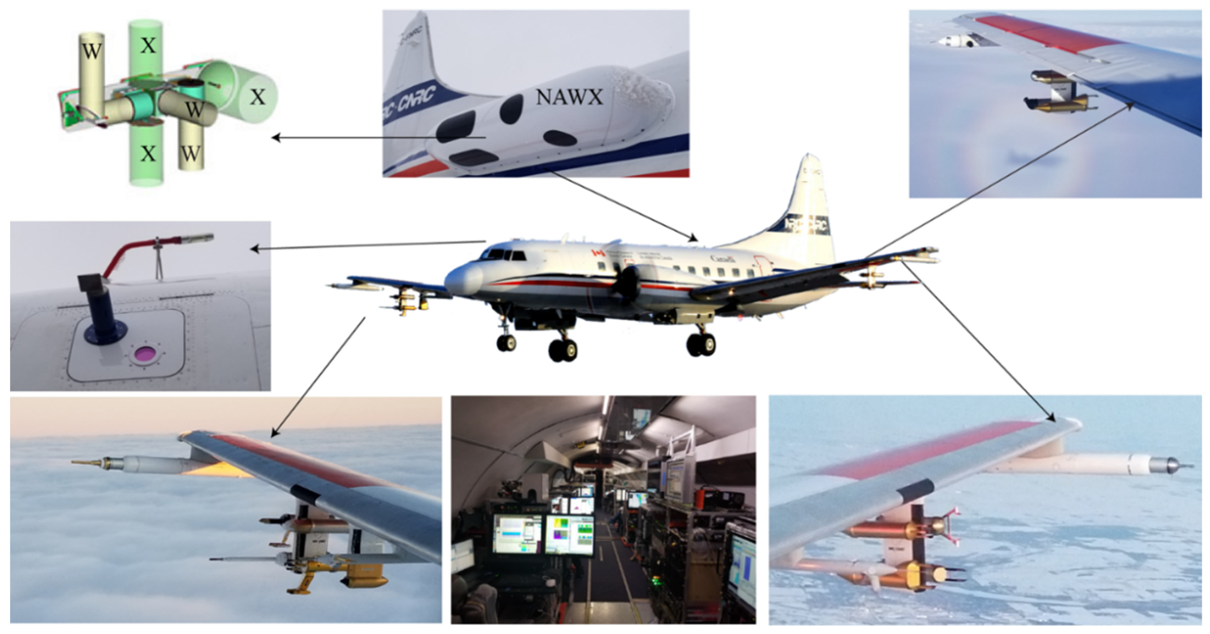
2.1. NRC Convair-580 Research Aircraft
2.1.1. Aircraft Instruments
Nevzorov
Rosemount Icing Detector
OAP and Scattering Probes
Rosemount Temperature Sensor
UHSAS
NAW
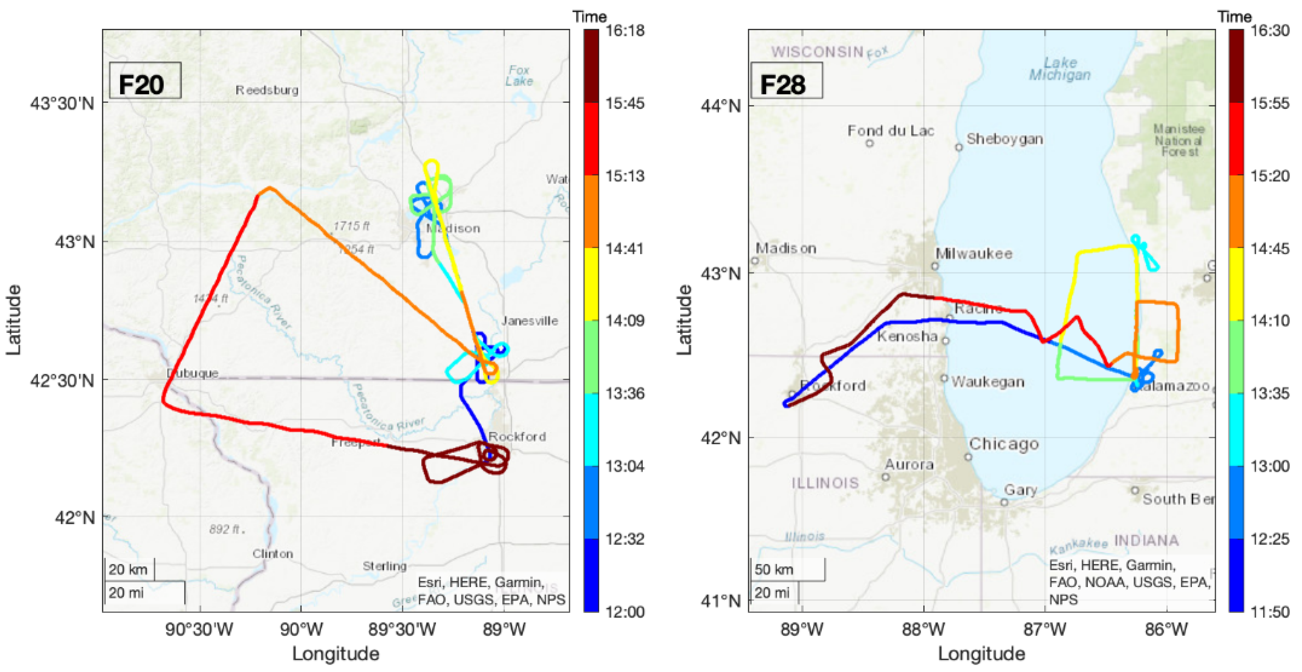
2.2. ICICLE Flight Campaign
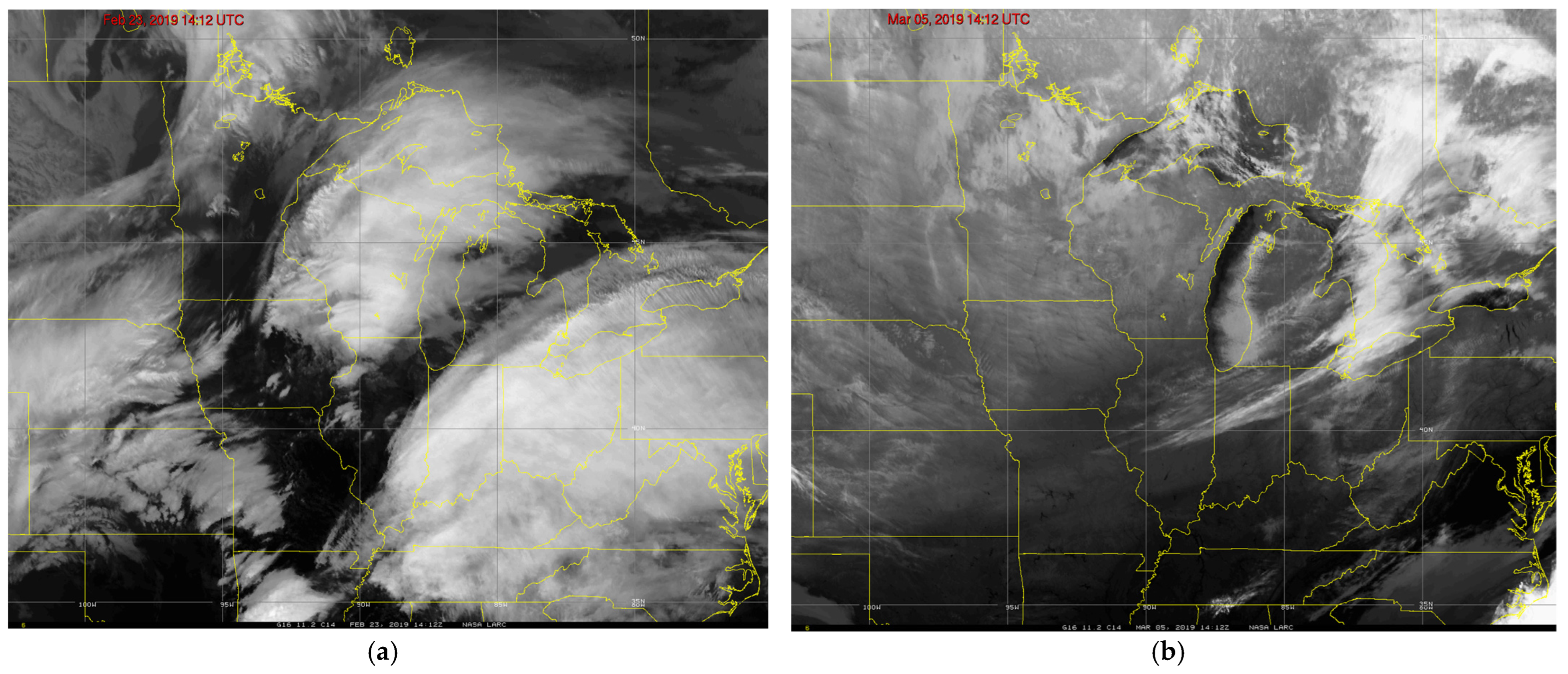
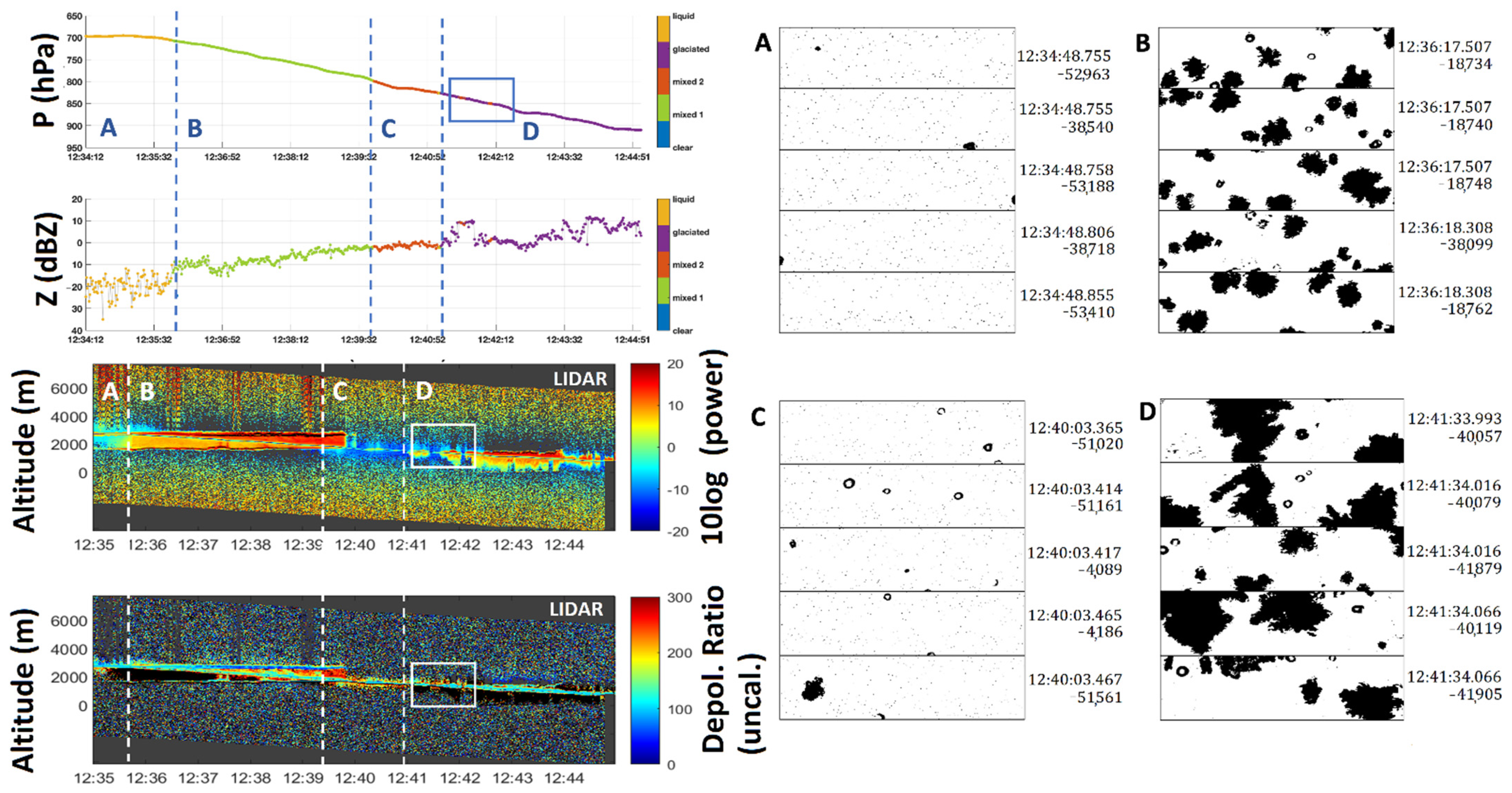
2.2.1. Flight 20, 23 February 2019
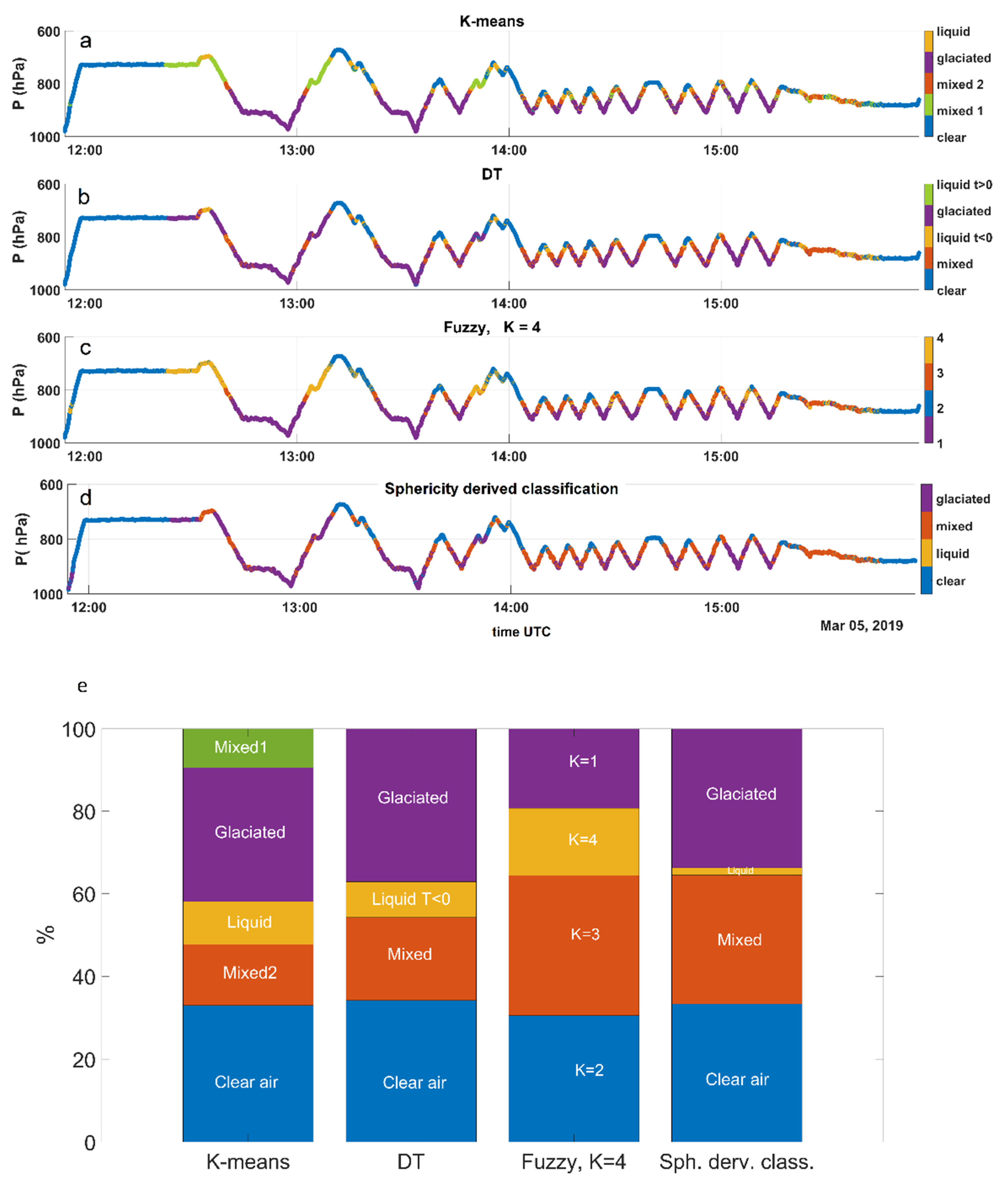
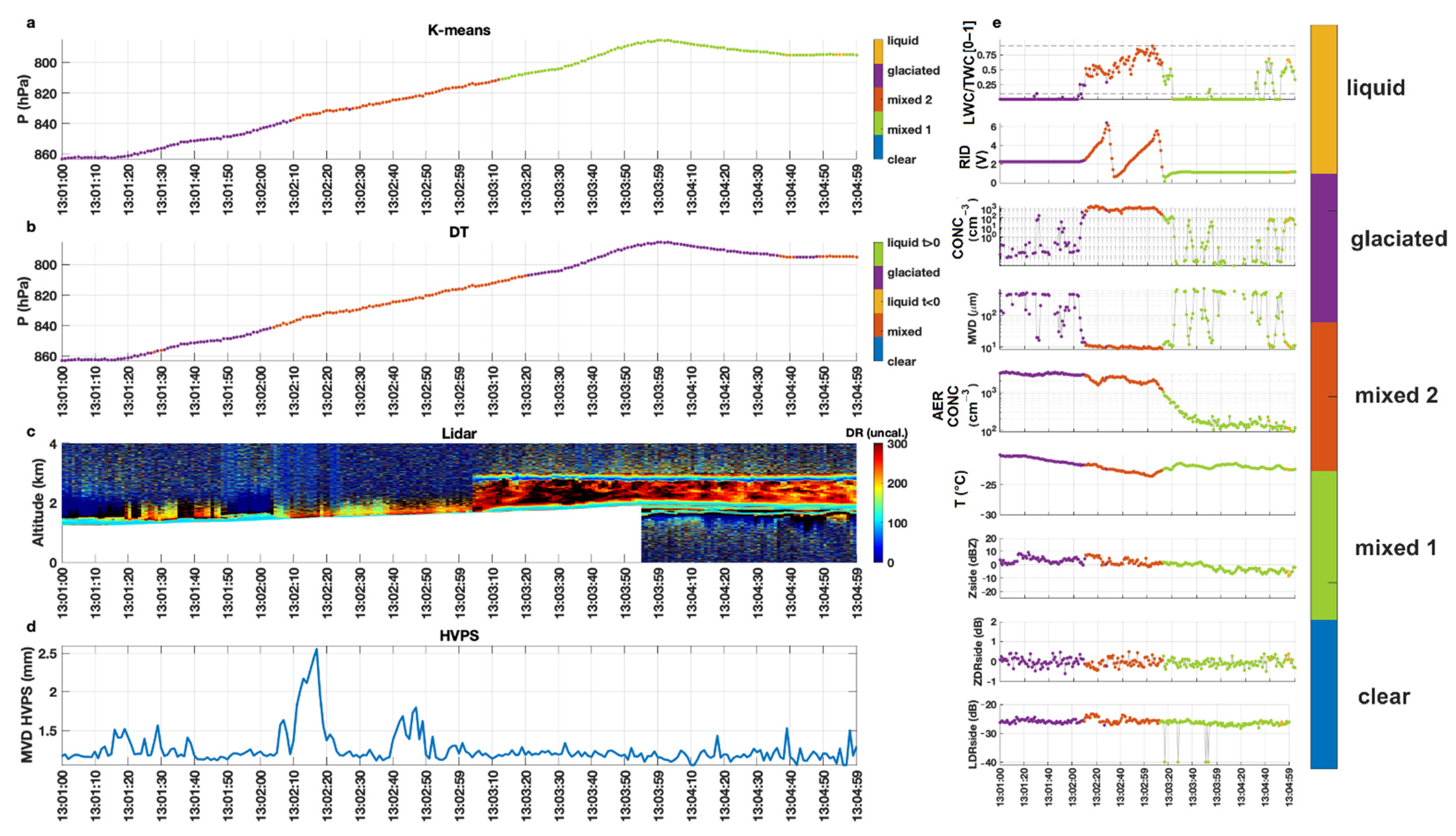
2.2.2. Flight 28, 5 March 2019
2.3. Classification Approaches
2.3.1. Clustering Methods
K-Means
Fuzzy Clustering
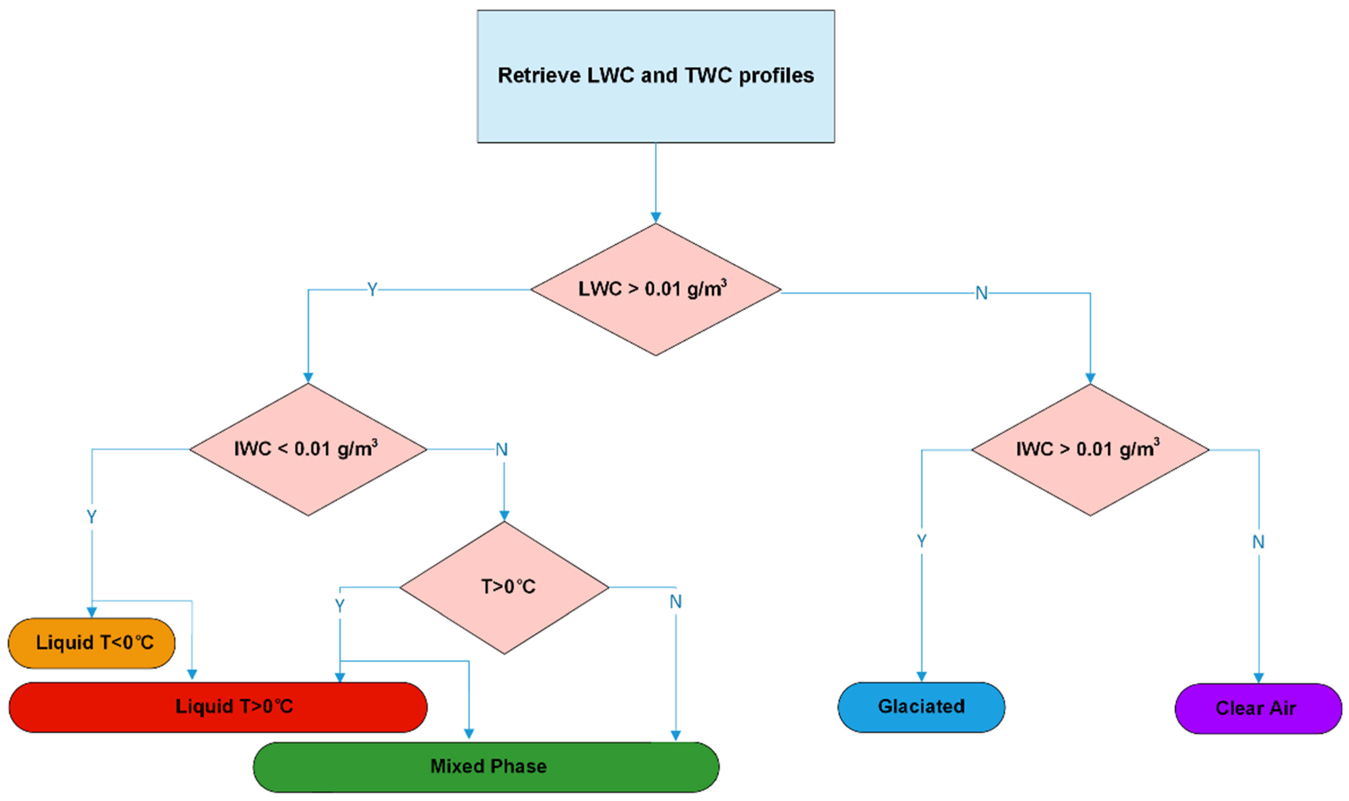
Decision Tree Dendrogram Classification Method
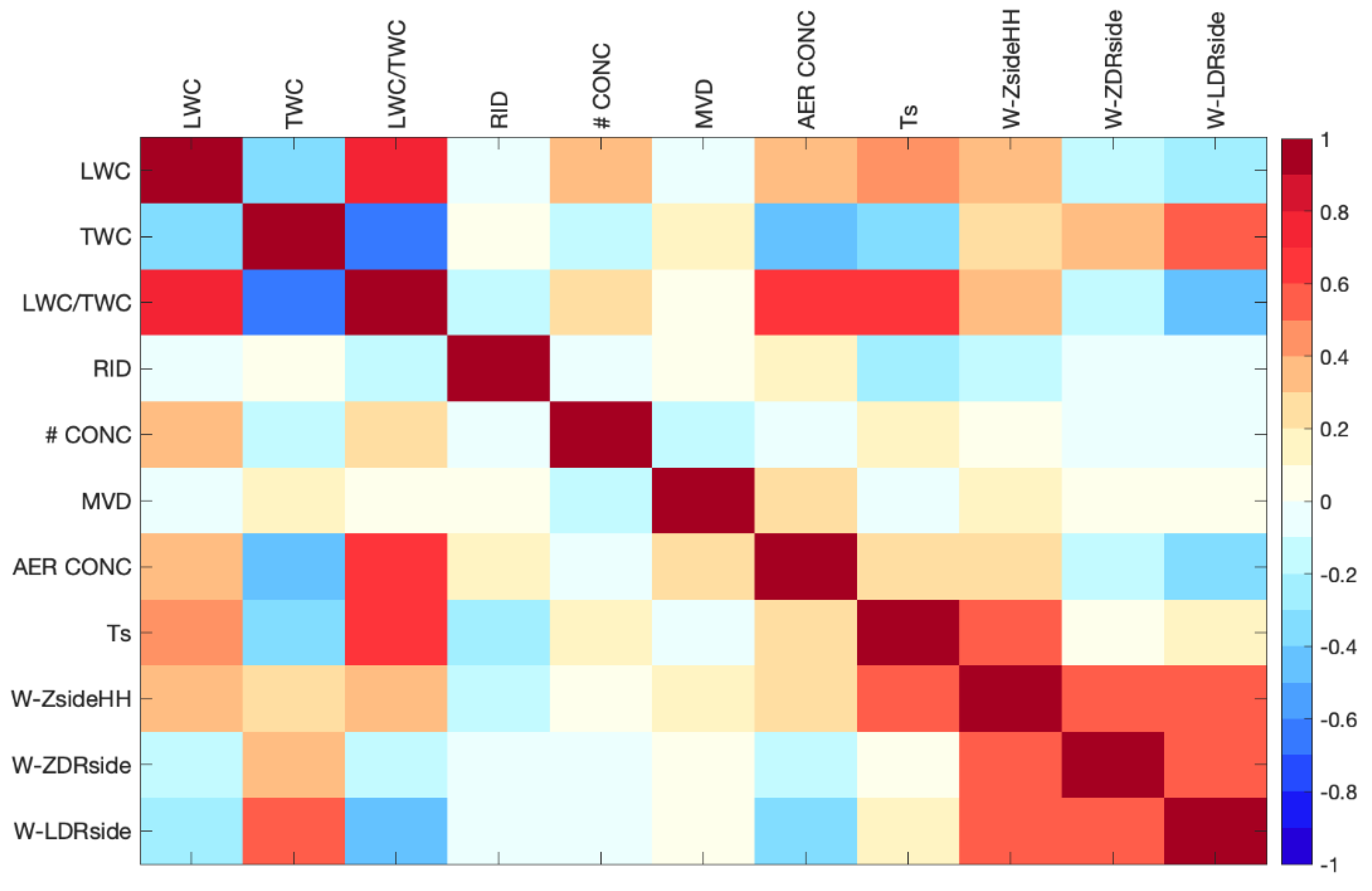
2.3.2. Data Preparation
3. Results
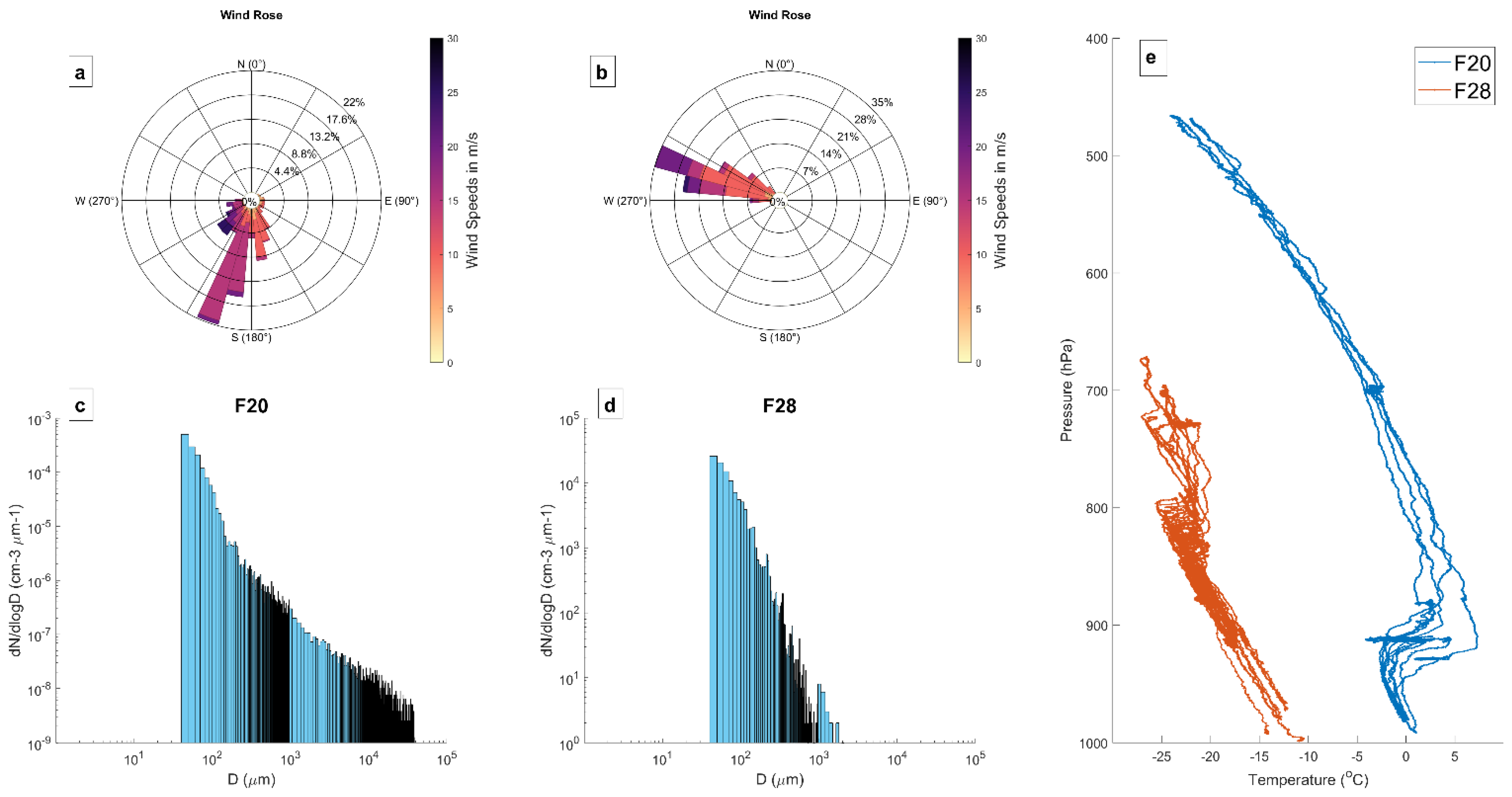
3.1. Variety of Conditions in Flight
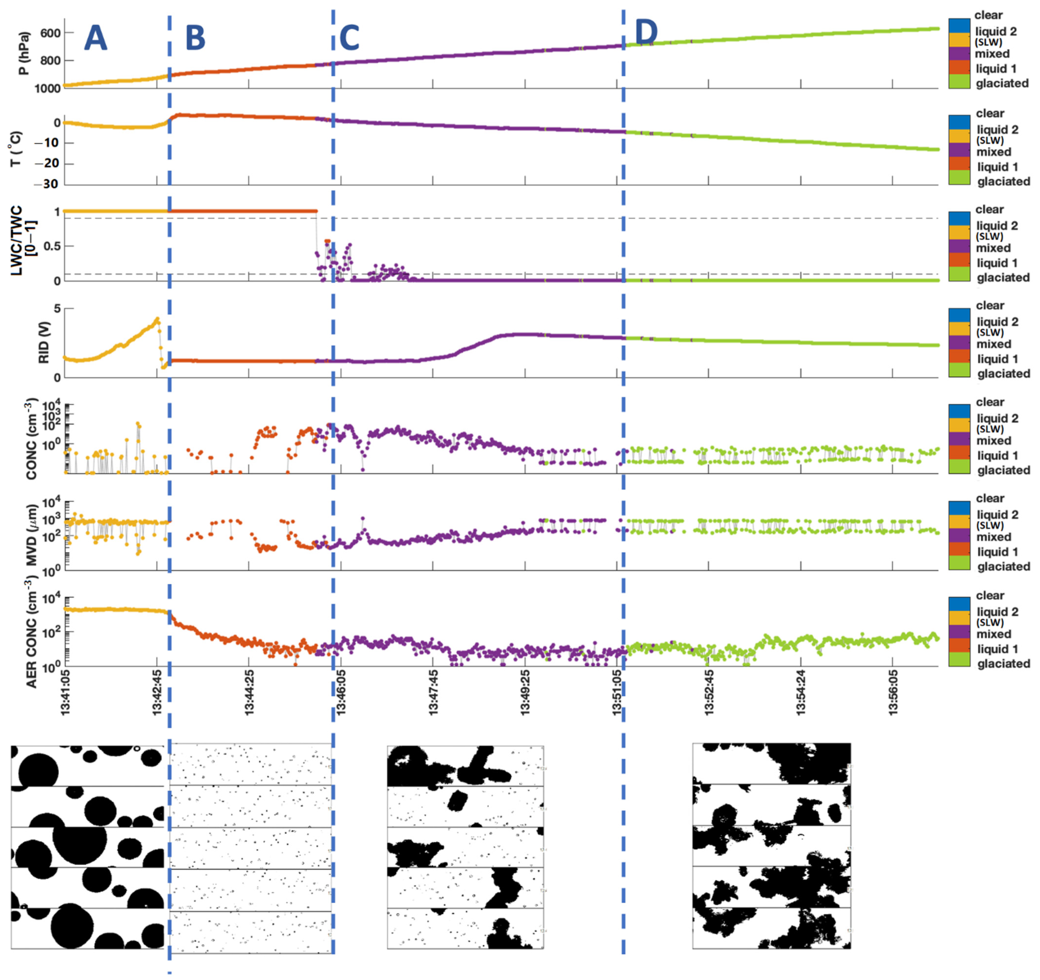
3.2. Flight 20
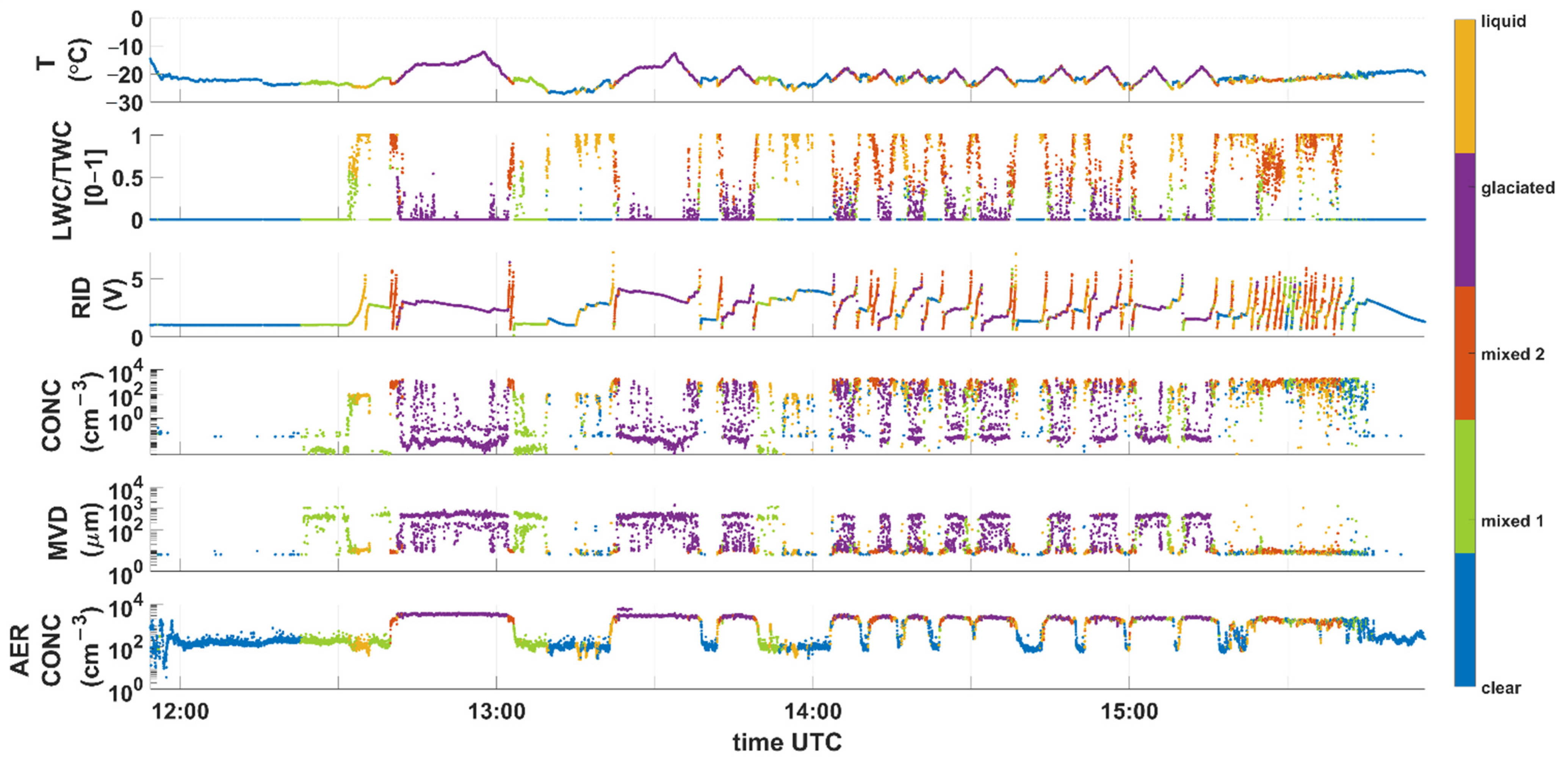
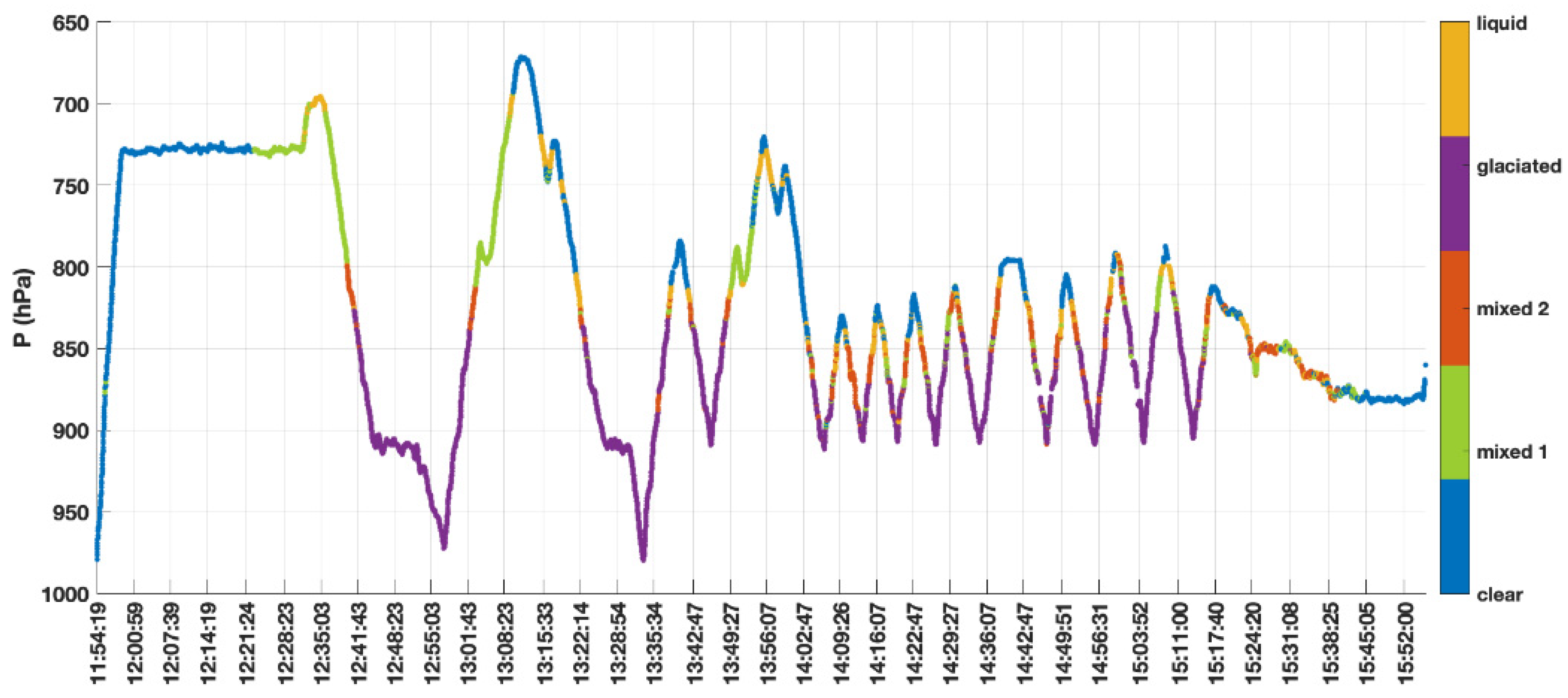
3.3. Flight 28
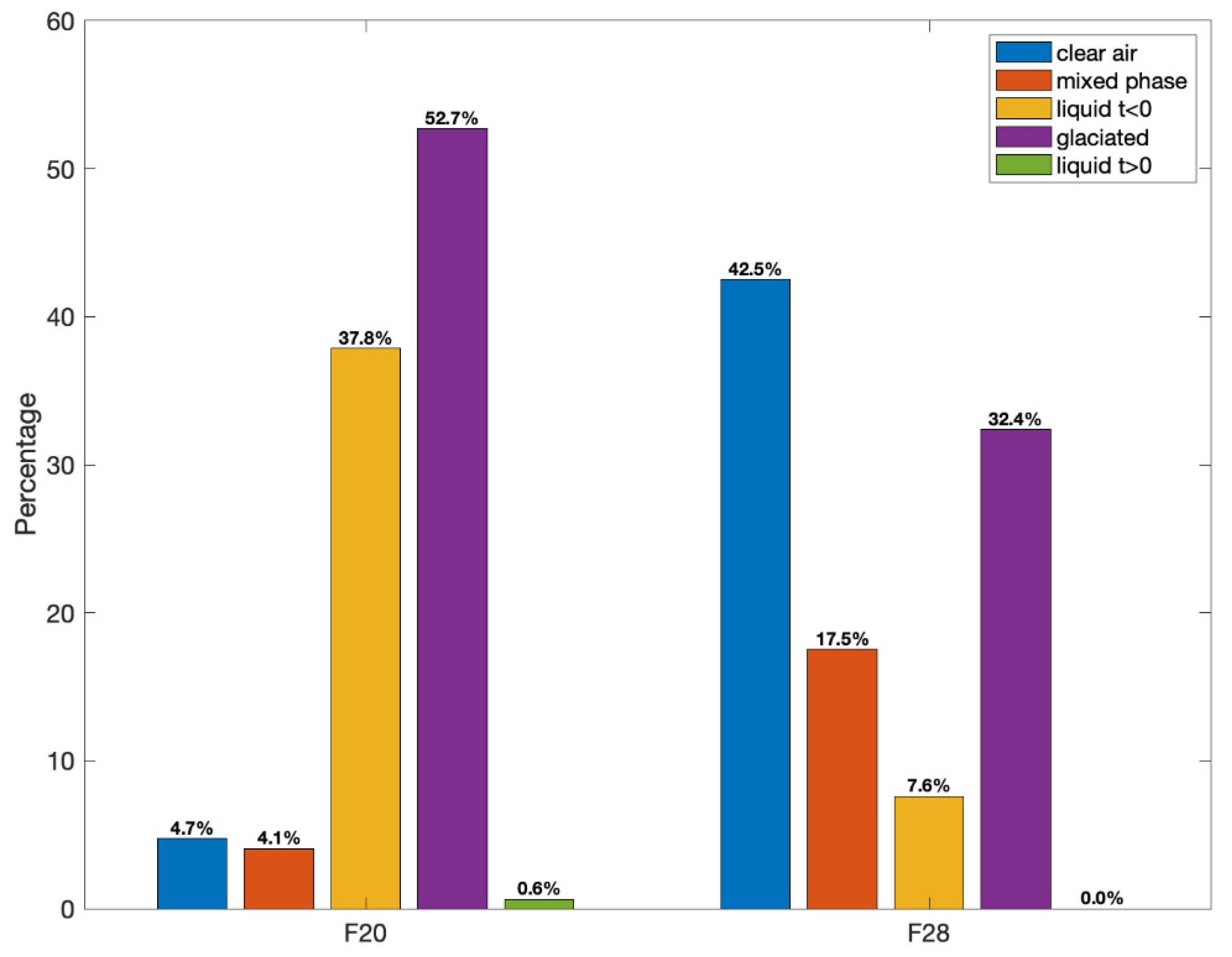
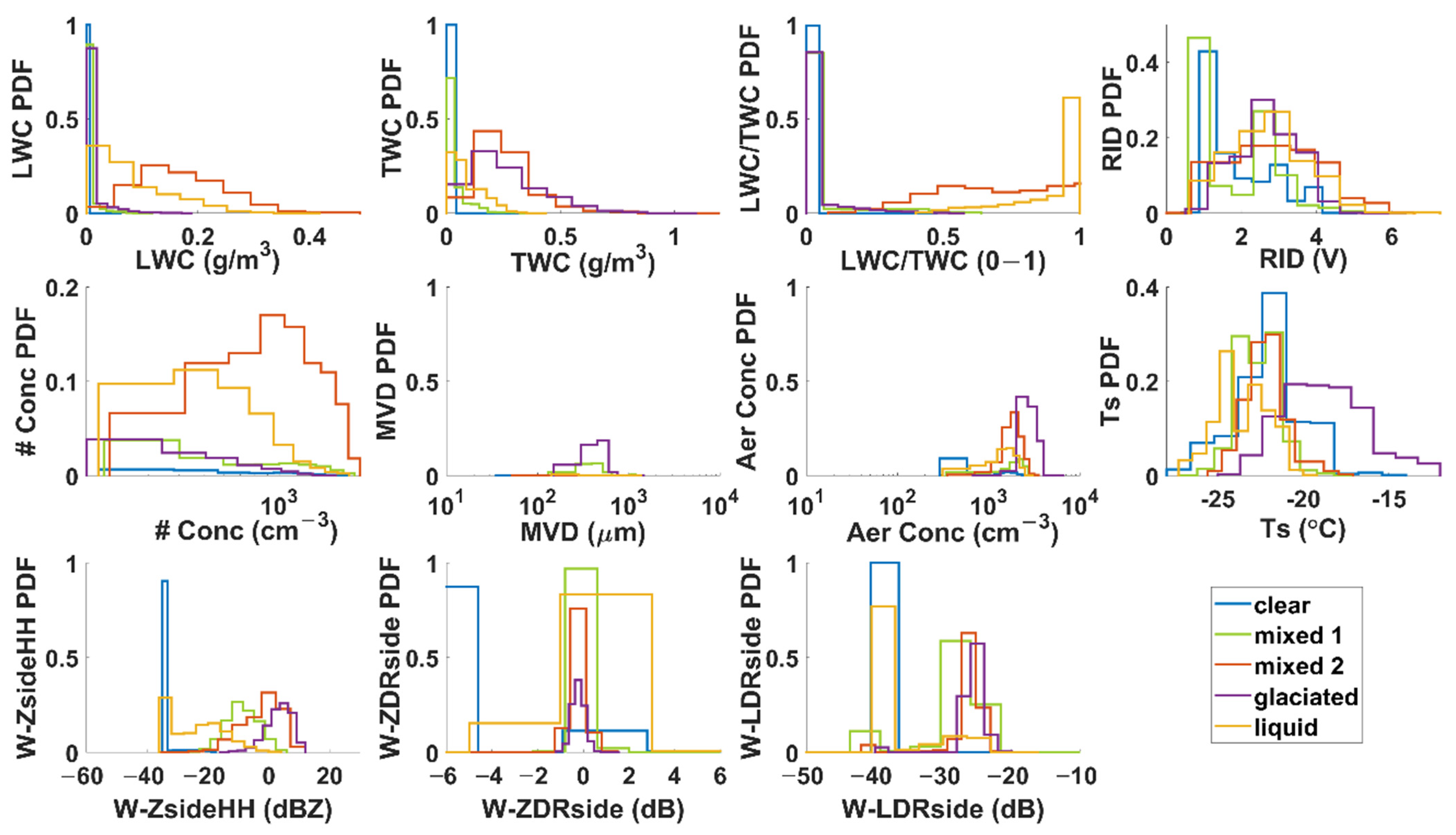
3.4. Classification Intercomparison
4. Discussion and Practical Applications
5. Conclusions
Author Contributions
Funding
Data Availability Statement
Acknowledgments
Conflicts of Interest
References
- Jayde, M.K.; Blickensderfer, B.; Guinn, T.; Kleber, J.L. The Effects of Display Type, Weather Type, and Pilot Experience on Pilot Interpretation of Weather Products. Atmosphere 2021, 12, 143. [Google Scholar] [CrossRef]
- Williams, E.R.; Donovan, M.F.; Smalley, D.J.; Hallowell, R.G.; Griffin, E.; Hood, K.T.; Bennett, B.J. The 2013 Buffalo Area Icing and Radar Study; Project Report ATC-419; MIT Lincoln Laboratory: Lexington, MA, USA, 2015. [Google Scholar]
- Williams, E.R.; Smalley, D.J.; Donovan, M.F. Recommendations for ICICLE and Other Future Icing Hazard Campaigns Based on Experience with In Situ Validation and NEXRAD Dual Polarimetric Radar Assessments of Icing Conditions; Document 43PM-Wx-0182; MIT Lincoln Laboratory: Lexington, MA, USA, 2018. [Google Scholar]
- Williams, E.R.; Donovan, M.F.; Smalley, D.J.; Kurdzo, J.M.; Bennett, B.J. The 2017 Buffalo Area Icing and Radar Study (BAIRS II); Report ATC-447; MIT Lincoln Laboratory: Lexington, MA, USA, 2020. [Google Scholar]
- DiVito, S.; Riley, J.; Landolt, S.D.; Bernestein, B.; Green, S.; Bracken, J. An Update of the Federal Aviation Administration Terminal Area Icing Weather Information for NextGen (TAIWIN) Project. In Proceedings of the 21st Conference on Aviation, Range, and Aerospace Meteorology, American Meteorological Society 101st Annual Meeting, 10.1, Virtual, 14 January 2021; Available online: https://ams.confex.com/ams/101ANNUAL/meetingapp.cgi/Paper/384097 (accessed on 1 January 2022).
- Öktem, R.; Romps, D.M. Prediction for cloud spacing confirmed using stereo cameras. J. Atmos. Sci. 2021, 78, 3717–3725. [Google Scholar] [CrossRef]
- Cesana, G.; Chepfer, H.; Winker, D.; Getzewich, B.; Cai, X.; Jourdan, O.; Mioche, G.; Okamoto, H.; Hagihara, Y.; Noel, V.; et al. Using in situ airborne measurements to evaluate three cloud phase products derived from CALIPSO. J. Geophys. Res. Atmos. 2016, 121, 5788–5808. [Google Scholar] [CrossRef] [Green Version]
- Hu, J.; Rosenfeld, D.; Zhu, Y.; Lu, X.; Carlin, J. Multi-channel Imager Algorithm (MIA): A novel cloud-top phase classification algorithm. Atmos. Res. 2021, 261, 105767. [Google Scholar] [CrossRef]
- Smith, W.L., Jr.; Minnis, P.; Fleeger, C.; Spangenberg, D.; Palikonda, R.; Nguyen, L. Determining the Flight Icing Threat to Aircraft with Single-Layer Cloud Parameters Derived from Operational Satellite Data. J. Appl. Meteorol. Climatol. 2012, 51, 1794–1810. [Google Scholar] [CrossRef]
- Doulgeris, K.-M.; Komppula, M.; Romakkaniemi, S.; Hyvärinen, A.-P.; Kerminen, V.-M.; Brus, D. In situ cloud ground-based measurements in the Finnish sub-Arctic: Intercomparison of three cloud spectrometer setups. Atmos. Meas. Tech. 2020, 13, 5129–5147. [Google Scholar] [CrossRef]
- McFarquhar, G.M.; Baumgardner, D.; Bansemer, A.; Abel, S.J.; Crosier, J.; French, J.; Rosenberg, P.; Korolev, A.V.; Schwarzoenboeck, A.; Leroy, D.; et al. Processing of Ice Cloud in Situ Data Collected by Bulk Water, Scattering, and Imaging Probes: Fundamentals, Uncertainties, and Efforts toward Consistency. Meteorol. Monogr. 2017, 58, 11.1–11.33. [Google Scholar] [CrossRef] [Green Version]
- Straka, J.M.; Zrnić, D.S.; Ryzhkov, A.V. Bulk Hydrometeor Classification and Quantification Using Polarimetric Radar Data: Synthesis of Relations. J. Appl. Meteorol. 2000, 39, 1341–1372. [Google Scholar] [CrossRef]
- Liu, H.; Chandrasekar, V. Classification of Hydrometeors Based on Polarimetric Radar Measurements: Development of Fuzzy Logic and Neuro-Fuzzy Systems, and In Situ Verification. J. Atmos. Ocean. Technol. 2000, 17, 140–164. [Google Scholar] [CrossRef]
- Korolev, A.V.; Isaac, G.A.; Cober, S.G.; Strapp, J.W.; Hallett, J. Microphysical characterization of mixed-phase clouds. Q. J. R. Meteorol. Soc. 2003, 129, 39–65. [Google Scholar] [CrossRef]
- D’Alessandro, J.J.; McFarquhar, G.M.; Wu, W.; Stith, J.L.; Jensen, J.B.; Rauber, R.M. Characterizing the occurrence and spatial heterogeneity of liquid, ice and mixed phase low-level clouds over the Southern Ocean using in situ observations acquired during SOCRATES. J. Geophys. Res. Atmos. 2021, 126, 11. [Google Scholar] [CrossRef]
- Holroyd, E.W. Some Techniques and Uses of 2D-C Habit Classification Software for Snow Particles. J. Atmos. Ocean. Technol. 1987, 4, 498–511. [Google Scholar] [CrossRef]
- Korolev, A.; Sussman, B. A Technique for Habit Classification of Cloud Particles. J. Atmos. Ocean. Technol. 2000, 17, 1048–1057. [Google Scholar] [CrossRef]
- Korolev, A. Reconstruction of the Sizes of Spherical Particles from Their Shadow Images. Part I: Theoretical Considerations. J. Atmos. Ocean. Technol. 2007, 24, 376–389. [Google Scholar] [CrossRef]
- Cober, S.G.; Isaac, G.A.; Korolev, A.V.; Strapp, J.W. Assessing Cloud-Phase Conditions. J. Appl. Meteorol. 2001, 40, 1967–1983. [Google Scholar] [CrossRef]
- Bernstein, B.; DiVito, S.; Riley, J.T.; Landolt, S.; Sims, D.; Haggerty, J.; Korolev, A.; Heckman, I.; Wolde, M.; Nichman, L.; et al. Overview of NRC Convair-580 In situ Flight Observations Made during ICICLE. In Proceedings of the 21st Conference on Aviation, Range, and Aerospace Meteorology, American Meteorological Society 101st Annual Meeting 10.4A, Virtual, 14 January 2021. [Google Scholar]
- Dilmi, M.D.; Mallet, C.; Barthes, L.; Chazottes, A. Data-driven clustering of rain events: Microphysics information derived from macro-scale observations. Atmos. Meas. Tech. 2017, 10, 1557–1574. [Google Scholar] [CrossRef] [Green Version]
- Belacel, N.; Hansen, P.; Mladenovic, N. Fuzzy J-Means: A New Heuristic for Fuzzy Clustering. Pattern Recognit. 2002, 35, 2193–2200. [Google Scholar] [CrossRef]
- He, S.; Belacel, N.; Chan, A.; Hamam, H.; Bouslimani, Y. A hybrid artificial fish swarm simulated annealing optimization algorithm for automatic identification of clusters. Int. J. Inf. Tech. Decis. 2016, 15, 949–974. [Google Scholar] [CrossRef]
- Bernstein, B.; DiVito, S.; Riley, J.T.; Landolt, S.; Haggerty, J.; Thompson, G.; Adriaansen, D.; Serke, D.; Kessinger, C.; Tessendorf, S.; et al. The In-Cloud Icing and Large-Drop Experiment Science and Operations Plans [DOT/FAA/TC-21/29]; Atlantic City International Airport, Federal Aviation Administration: Egg Harbor Township, NJ, USA, 2021. [Google Scholar] [CrossRef]
- Wolde, M.; Nguyen, C.; Korolev, A.; Bastian, M. Characterization of the Pilot X-band radar responses to the HIWC environment during the Cayenne HAIC-HIWC 2015 Campaign. In Proceedings of the 8th AIAA Atmospheric and Space Environments Conference, AIAA 2016-4201, Washington, DC, USA, 13–17 June 2016; Available online: https://arc.aiaa.org/doi/10.2514/6.2016-4201 (accessed on 1 January 2022).
- Nichman, L.; Bliankinshtein, N.; Wolde, M.; Davison, C.; Fuleki, D.; Orchard, D.; Nolan, C.; Keating, D.; Jackson, D.; Olvhamma, S.; et al. Advanced techniques for airborne measurements tested onboard NRC’s Convair-580 Aircraft. In Proceedings of the International Conference on Clouds and Precipitation (ICCP), Pune, India, 2–6 August 2021; Available online: https://tinyurl.com/iccpconvair (accessed on 1 January 2022).
- Korolev, A.V.; Strapp, J.W.; Isaac, G.A.; Nevzorov, A.N. The Nevzorov Airborne Hot-Wire LWC-TWC Probe: Principle of Operation and Performance Characteristics. J. Atmos. Ocean. Technol. 1998, 15, 1495–1510. [Google Scholar] [CrossRef]
- Baumgardner, D.; Rodi, A. Laboratory and wind tunnel evaluations of the Rosemount Icing Detector. J. Atmos. Ocean. Technol. 1989, 6, 971–979. [Google Scholar] [CrossRef]
- Heymsfield, A.J.; Miloshevich, L.M. Evaluation of Liquid Water Measuring Instruments in Cold Clouds Sampled during FIRE. J. Atmos. Ocean. Technol. 1989, 6, 378–388. [Google Scholar] [CrossRef]
- Cober, S.G.; Isaac, G.A.; Korolev, A.V. Assessing the Rosemount icing detector with in situ measurements. J. Atmos. Ocean. Technol. 2001, 18, 515–528. [Google Scholar] [CrossRef]
- Nguyen, C.M.; Wolde, M.; Battaglia, A.; Nichman, L.; Bliankinshtein, N.; Haimov, S.; Bala, K.; Schuettemeyer, D. Coincident in situ and triple-frequency radar airborne observations in the Arctic. Atmos. Meas. Tech. 2022, 15, 775–795. [Google Scholar] [CrossRef]
- Baumgardner, D.; Abel, S.J.; Axisa, D.; Cotton, R.; Crosier, J.; Field, P.; Gurganus, C.; Heymsfield, A.; Korolev, A.V.; Krämer, M.; et al. Cloud Ice Properties: In Situ Measurement Challenges. Meteorol. Monogr. 2017, 58, 9.1–9.23. [Google Scholar] [CrossRef] [Green Version]
- Stickney, T.M.; Shedlov, M.W.; Thompson, D.I. Goodrich Total Temperature Sensors; Technical Report 5755; Revision, C., Ed.; Rosemount Aerospace Inc.: Burnsville, MN, USA, 1994. [Google Scholar]
- Droplet Measurement Technologies. Ultra-High Sensitivity Aerosol Spectrometer (UHSAS), Operator Manual, DOC-0210, Rev E-4; Software Version 4.1.0; Droplet Measurement Technologies: Longmont, CO, USA, 2013. [Google Scholar]
- Wolde, M.; Pazmany, A. NRC dual-frequency airborne radar for atmospheric research. In Proceedings of the 32nd Conference on Radar Meteorology, Albuquerque, NM, USA, 24–29 October 2005. P1R.9. [Google Scholar]
- Baibakov, K.; Wolde, M.; Nguyen, C.; Korolev, A.; Wang, Z.; Wechsler, P. Performance of a compact elastic 355 nm airborne lidar in tropical and mid-latitude clouds. In Proceedings of the SPIE 10006, Lidar Technologies, Techniques, and Measurements for Atmospheric Remote Sensing XII, 100060C, Edinburgh, UK, 24 October 2016. [Google Scholar] [CrossRef]
- Lawson, R.P.; Baker, B.A.; Schmitt, C.G.; Jensen, T.L. An overview of microphysical properties of Arctic clouds observed in May and July during FIRE ACE. J. Geophys. Res. 2001, 106, 14989–15014. [Google Scholar] [CrossRef] [Green Version]
- Rugg, A.; Bernstein, B.C.; Haggerty, J.A.; Korolev, A.; Nguyen, C.; Wolde, M.; Heckman, I.; DiVito, S. High Ice Water Content Conditions Associated with Wintertime Elevated Convection in the Midwest. J. Appl. Meteorol. Climatol. 2022, 61, 559–575. [Google Scholar] [CrossRef]
- Xu, D.; Tian, Y. A Comprehensive Survey of Clustering Algorithms. Ann. Data. Sci. 2015, 2, 165–193. [Google Scholar] [CrossRef] [Green Version]
- Belacel, N.; Wang, C.; Cupelovic-Culf, M. Clustering: Unsupervised Learning in Large Biological Data. In Statistical Bioinformatics: A Guide for Life and Biomedical Science Researchers; Wiley Online Library: Hoboken, NJ, USA, 2010; Chapter 5; pp. 89–127. [Google Scholar] [CrossRef]
- Bezdek, J.C. Pattern Recognition with Fuzzy Objective Function Algorithms; Plenum Press: New York, NY, USA, 1981. [Google Scholar] [CrossRef]
- Lloyd, S.P. Least Squares Quantization in PCM. IEEE Trans. Inf. Theory 1982, 28, 129–137. [Google Scholar] [CrossRef] [Green Version]
- David, A.; Vassilvitskii, S. K-Means++: The Advantages of Careful Seeding. In Proceedings of the Eighteenth Annual ACM-SIAM Symposium on Discrete Algorithms; Society for Industrial and Applied Mathematics: Philadelphia, PA, USA, 2007; pp. 1027–1035. [Google Scholar] [CrossRef]
- Fränti, P.; Sieranoja, S. How much can k-means be improved by using better initialization and repeats? Pattern Recognit. 2019, 93, 95–112. [Google Scholar] [CrossRef]
- Tibshirani, R.; Walther, G.; Hastie, T. Estimating the number of clusters in a data set via the gap statistic. J. R. Stat. Soc. Ser. B (Stat. Methodol.) 2001, 63, 411–423. [Google Scholar] [CrossRef]
- Belacel, N.; Čuperlović-Culf, M.; Laflamme, M.; Ouellette, R. Fuzzy J-Means and VNS methods for clustering genes from microarray data. Bioinformatics 2004, 22, 1690–1701. [Google Scholar] [CrossRef] [PubMed] [Green Version]
- Duda, R.; Hart, P.; Stork, D. Pattern Classification, 2nd ed.; Wiley: New York, NY, USA, 2001; ISBN 978-0-471-05669-0. [Google Scholar]
- Brodley, C.E.; Utgoff, P.E. Multivariate Decision Trees. Mach. Learn. 1995, 19, 45–77. [Google Scholar] [CrossRef] [Green Version]
- Kohavi, R.; John, G. Wrappers for feature selection. Artif. Intell. 1997, 97, 273–324. [Google Scholar] [CrossRef] [Green Version]
- Blum, A.; Langley, P. Selection of relevant features and examples in machine learning. Artif. Intell. 1997, 97, 245–271. [Google Scholar] [CrossRef] [Green Version]
- Guyon, I.; Elisseeff, A. An introduction to variable and feature selection. J. Mach. Learn. Res. 2003, 3, 1157–1182. [Google Scholar] [CrossRef]
- Kreidenweis, S.M.; Petters, M.; Lohmann, U. 100 Years of Progress in Cloud Physics, Aerosols, and Aerosol Chemistry Research. Meteorol. Monogr. 2019, 59, 11.1–11.72. [Google Scholar] [CrossRef]
- Fontaine, E.; Schwarzenboeck, A.; Leroy, D.; Delanoë, J.; Protat, A.; Dezitter, F.; Strapp, J.W.; Lilie, L.E. Statistical analysis of ice microphysical properties in tropical mesoscale convective systems derived from cloud radar and in situ microphysical observations. Atmos. Chem. Phys. 2020, 20, 3503–3553. [Google Scholar] [CrossRef] [Green Version]
- Yachao, H.; McFarquhar, G.M.; Wu, W.; Huang, Y.; Schwarzenboeck, A.; Protat, A.; Korolev, A.; Rauber, R.M.; Wang, H. Dependence of Ice Microphysical Properties on Environmental Parameters: Results from HAIC-HIWC Cayenne Field Campaign. J. Atmos. Sci. 2021, 78, 2957–2981. [Google Scholar] [CrossRef]
- Korolev, A.; Field, P.R. Assessment of the performance of the inter-arrival time algorithm to identify ice shattering artifacts in cloud particle probe measurements. Atmos. Meas. Tech. 2015, 8, 761–777. [Google Scholar] [CrossRef] [Green Version]
- Wu, W.; McFarquhar, G.M. On the Impacts of Different Definitions of Maximum Dimension for Nonspherical Particles Recorded by 2D Imaging Probes. J. Atmos. Ocean. Technol. 2016, 33, 1057–1072. [Google Scholar] [CrossRef]
- Mazin, I.P.; Korolev, A.V.; Heymsfield, A.; Isaac, G.A.; Cober, S.G. Thermodynamics of Icing Cylinder for Measurements of Liquid Water Content in Supercooled Clouds. J. Atmos. Ocean. Technol. 2001, 18, 543–558. [Google Scholar] [CrossRef]
- Schwarzenboeck, A.; Mioche, G.; Armetta, A.; Herber, A.; Gayet, J.-F. Response of the Nevzorov hot wire probe in clouds dominated by droplet conditions in the drizzle size range. Atmos. Meas. Tech. 2009, 2, 779–788. [Google Scholar] [CrossRef] [Green Version]
- Korolev, A.; McFarquhar, G.; Field, P.R.; Franklin, C.; Lawson, P.; Wang, Z.; Williams, E.; Abel, S.J.; Axisa, D.; Borrmann, S.; et al. Mixed-Phase Clouds: Progress and Challenges. Meteorol. Monogr. 2017, 58, 5.1–5.50. [Google Scholar] [CrossRef]
- Sadouk, L. CNN Approaches for Time Series Classification. In Time Series Analysis-Data, Methods, and Applications; Ngan, C.-K., Ed.; IntechOpen: London, UK, 2019. [Google Scholar] [CrossRef] [Green Version]
- Cober, S.G.; Isaac, G.A.; Strapp, J.W. Aircraft Icing Measurements in East Coast Winter Storms. J. Appl. Meteorol. Climatol. 1995, 34, 88–100. [Google Scholar] [CrossRef]


| # | Selected Parameter | Description | Source Instrument |
|---|---|---|---|
| 1 | LWC [g m−3] | Bulk in situ Cloud microphysics | Nevzorov |
| 2 | TWC [g m−3] | Bulk in situ Cloud microphysics | Nevzorov |
| 3 | LWC/TWC [a.u.] | Bulk in situ Cloud microphysics | Nevzorov |
| 4 | Icing periods [Hz] | Bulk in situ Cloud microphysics | Rosemount Icing Detector |
| 5 | Number concentration [cm−3] | Single particle in situ Cloud microphysics | OAP & Scattering probes |
| 6 | MVD [µm] | Single particle in situ Cloud microphysics | OAP & Scattering probes |
| 7 | Static temperature [°C] | Atmospheric state | Rosemount temperature sensor |
| 8 | Aerosol number concentration [cm−3] | Aerosol | UHSAS |
| 9 | Radar reflectivity [dBZ] | Remote sensing | NAW |
| 10 | ZDR [dB] | Remote sensing | NAW |
| 11 | LDR [dB] | Remote sensing | NAW |
Publisher’s Note: MDPI stays neutral with regard to jurisdictional claims in published maps and institutional affiliations. |
© 2022 by the authors. Licensee MDPI, Basel, Switzerland. This article is an open access article distributed under the terms and conditions of the Creative Commons Attribution (CC BY) license (https://creativecommons.org/licenses/by/4.0/).
Share and Cite
Shakirova, A.; Nichman, L.; Belacel, N.; Nguyen, C.; Bliankinshtein, N.; Wolde, M.; DiVito, S.; Bernstein, B.; Huang, Y. Multivariable Characterization of Atmospheric Environment with Data Collected in Flight. Atmosphere 2022, 13, 1715. https://doi.org/10.3390/atmos13101715
Shakirova A, Nichman L, Belacel N, Nguyen C, Bliankinshtein N, Wolde M, DiVito S, Bernstein B, Huang Y. Multivariable Characterization of Atmospheric Environment with Data Collected in Flight. Atmosphere. 2022; 13(10):1715. https://doi.org/10.3390/atmos13101715
Chicago/Turabian StyleShakirova, Aliia, Leonid Nichman, Nabil Belacel, Cuong Nguyen, Natalia Bliankinshtein, Mengistu Wolde, Stephanie DiVito, Ben Bernstein, and Yi Huang. 2022. "Multivariable Characterization of Atmospheric Environment with Data Collected in Flight" Atmosphere 13, no. 10: 1715. https://doi.org/10.3390/atmos13101715