Article

A Study to Explore the Dew Condensation Potential of Cars

1
Scientific and Technical Faculty, Università di Corsica Pasquale Paoli, Avenue du 9 Septembre, BP 52, 20250 Corte, France
2
International Organization for Dew Utilization (OPUR), 2 Rue Verderet, 75016 Paris, France
3
Instituto de Investigación Multidisciplinario en Ciencia y Tecnología, Universidad de La Serena, Benavente 980, La Serena 1720170, Chile
4
Physique et Mécanique des Milieux Hétérogènes, CNRS, ESPCI Paris—PSL University, Sorbonne Université, Sorbonne Paris Cité, 10 Rue Vauquelin, 75005 Paris, France
*
Author to whom correspondence should be addressed.
Atmosphere 2022, 13(1), 65; https://doi.org/10.3390/atmos13010065
Submission received: 7 December 2021 / Revised: 22 December 2021 / Accepted: 27 December 2021 / Published: 30 December 2021
(This article belongs to the Special Issue Feature Papers in Atmosphere Science)

Abstract

:
The metal surfaces of a car exhibit favorable properties for the passive condensation of atmospheric water. Under certain nocturnal climatic conditions (high relative humidity, weak windspeed, and total nebulosity), dew is often observed on cars, and it is appropriate to ask the question of using a vehicle as a standard condenser for estimating the dew yield. In order to see whether cars can be used as reference dew condensers, we report a detailed study of radiative cooling and dew formation on cars in the presence of radiating obstacles and for various windspeeds. Measurements of temperature and condensed dew mass on different car parts (rooftop, front and back hoods, windshield, lateral and back windows, inside and outside air) are compared with the same data obtained on a horizontal, thermally isolated planar film. The paper concludes that heat transfer coefficients, evaluated from temperature and dew yield measurements, are found nearly independent of windspeed and tilt angles. Moreover, this work describes the relation between cooling and dew condensation with the presence or not of thermal isolation. This dependence varies with the surface tilt angle according to the angular dependence of the atmosphere radiation. This work also confirms that cars can be used to estimate the dew yields in a given site. A visual observation scale h = Kn, with h the dew yield (mm) and n = 0, 1 2, 3 an index, which depends whether dew forms or not on rooftop, windshield, and lateral windows, is successfully tested with 8 different cars in 5 sites with three different climates, using K = (0.067 ± 0.0036) mm·day−1.

1. Introduction

Natural dew is a ubiquitous phenomenon, which can be encountered at night in many places of the world when the conditions for its formation are met (clear sky, high relative humidity, low windspeed). Dew has been long studied by agrometeorologists for its impact in agriculture [1,2,3], positive to bring moisture to the plants, negative to foster fungal diseases. Dew water was more recently recognized as a supplementary source of fresh water due to its interesting chemical and biological qualities [4,5,6]. As a matter of fact, over the past decades, dew and the conditions of its formation have been the subject of numerous studies. One notes, in particular, the evaluation of its potential in several sites around the world under different climates [6,7,8].
Recent studies [9,10] show the impact of observed climate change on extreme nighttime and daytime temperatures. The main consequences of these temperature increases will be larger evapotranspiration, a greater presence of humidity in the air leading to prolonged dryness of the soils. The impact of global change on dew condensation potential has been evaluated for the Mediterranean basin [11]. It concluded to a decline in dew yield.
To date, the dew potential of a site is not available in national meteorological databases. It can be, however, estimated by physical models using meteorological data and/or radiometric measurements when available or by in situ measurements requiring the installation of a dew condensing device over a given time period. Dew measurements are performed by different techniques based on weighing, imaging, electric conductivity, capacitance (for reviews, see [4,6,12]). Physical models and empirical models for evaluating dew condensation volume are generally based on an energy balance equation. However, some are dependent on meteo parameters such as atmosphere radiation or windspeed at different heights, which are available only in a few meteorological stations. Neural network methods are useful but need preliminary measurements data [13]. Satellite data and geographical information systems were also tentatively used, but the relation to obtaining dew yield from the data remained unclear [14].
Concerning dew measurements, it was noticed that the observation of dew forming on the rooftop, windshield, and lateral windows of cars could be used to determine the local dew yield [15]. It is indeed a current observation that dew specifically condenses on car surfaces. Cars have geometric and material characteristics that promote dew formation on their outer surface when the weather conditions are suitable. A car is a metal shell with stagnant air inside and thermally isolated from the ground; cars have high-infrared emissivity exterior paints, which encourage dew formation by radiative cooling when exposed to a clear night sky with high relative humidity. In addition, when wet, the surface’s emissivities become close to water emissivity (0.98 in the atmospheric window [3]), which makes car surfaces near blackbodies.
The fact that nearly all cars exhibit similar geometrical and thermal characteristics on three specific parts (horizontal isolated rooftop, non-isolated, near-30° tilted windshield, and non-isolated, near-vertical lateral windows) and are used in nearly all parts of the world make particularly interesting the observation of dew formation at the sunrise as a proxy for quantitative dew measurements [15]. A dew intensity scale is defined by a 4 level observation index n = 0, 1, 2, 3, 0 for no dew, 1 for dew on the rooftop, 2 for dew on the rooftop and windshield, and 3 for dew on the rooftop, windshield, and side windows. Five types of cars in three different locations were concerned, and dew volume was measured on the rooftop of two of them. A relation was shown between the daily cumulative dew yield h, corresponding to what would have been measured on a reference, thermally isolated, planar 1 × 1 m² condenser, inclined 30° from horizontal, and n:
h = K n
It was found K = (0.067 ± 0.02) mm·day−1. It follows from this relation that anybody can estimate anywhere the quantity of condensed water by the daily observation at sunrise of dew forming (or not forming) on a car.
Other parts of a car can be used as dew condensing surfaces, and the corresponding dew condensation can be studied with respect to external meteorological conditions such as air temperature Ta, air dew point temperature Td, sky emissivity εs, windspeed V, and wind direction Dir V. For this purpose, the behavior of surface parameters important in dew formation, such as, e.g., condensing surface temperature Tc, orientation with wind, tilt angle with horizontal φ, skyview SV have to be investigated (Figure 1). The different parts of a car under given meteorological conditions indeed depend on several factors: emissivity εc of the condensing surface, tilt angle φ with horizontal for the dependence of radiative deficit with the angle-dependent sky emissivity, angular view α of obstacles, which emits IR radiation and limit the skyview, relative angle with respect to wind direction (forced air flow) and vertical direction (natural thermal convection), presence or absence of underneath thermal isolation.
In addition to the above factors, dew condensation is known to depend on the density of nucleation sites (see, e.g., Ref. [6]). Nucleation sites are sites where the surface energy of water droplets is lowered thanks to geometrical discontinuities (e.g., scratches) or chemical impurities. The fact that condensing surfaces are located outdoor ensures a high density of geometrical and chemical defects, thus a high density of nucleation sites. It has to be noted that the surface energy of car surfaces, which determines the water drop contact angle, does not intervene in the mean condensation rate (see Equations (38) and (41)). It has, however, great importance in the statistical properties of the drop pattern and the efficiency of water collection by gravity [6], which nevertheless is not the object of the present study.
It is the object of this paper to investigate the condensing behavior of the different parts of a car and analyze the results in terms of heat and mass transfer coefficients and angle-dependent radiation deficit. In addition to performing measurement of dew mass and recording the main meteorological parameters locally, temperature measurements on the rooftop, front hood, back hood, windshield, side, and back window are carried out and compared to a horizontal, thermally isolated reference foil condenser. Three different cars and two different locations (Ajaccio, France and Valparaiso, Chile) were considered, with time duration ranging between 1 to 103 days. The main results were concerned with (i) the dependence of the cooling efficiency with surface tilt angle and obstacle view angle as measured by the difference TcTa, (ii) the dew yield, directly measured or evaluated through the measured supersaturation TcTd or from an energy model, (iii) the evaluation from (i) and (ii) of the heat and mass transfer coefficients and (iv) the validation of Equation (1).
The paper is organized as follows. measurements and methods are initially described in the first section. The following section is devoted to the evaluation of surface temperatures as a function of the angle-dependent radiation deficit. Results and discussions follow concerning surfaces temperature measurements as a function of wind characteristics. Then the estimation of the dew yield from meteorological data and direct measurements is compared with the visual observation scale n.

2. Measurements and Methods

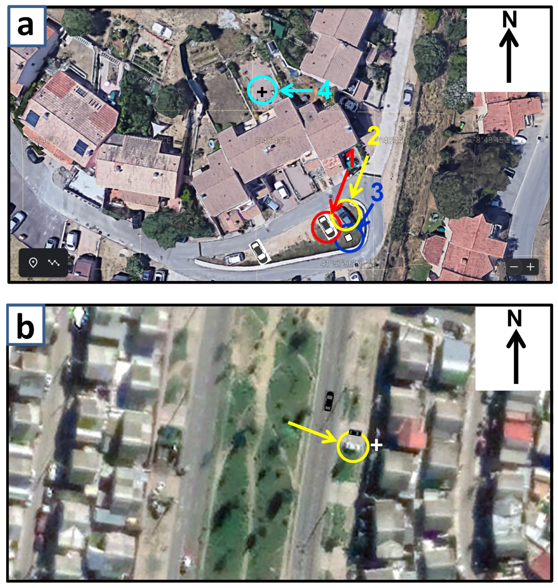
2.1. Measurement Sites

The test locations, Ajaccio (France) and Valparaiso (Chile) exhibit 2 different Köppen–Geiger’s classification climates (Am for Ajaccio and Csb for Valaparaiso). In addition to their dissimilarities in elevation and localization in 2 different hemispheres and the fact that one site is an island and the other a continental site, both experimental locations show significant meteorological differences (e.g., total rainfall precipitations).

2.1.1. Ajaccio

The main experimental site (Figure 2) was located 8 km from Ajaccio (Corsica island, France), on the residential district called Sarrola Carcopino (53 m asl elevation, 8°48′43″ E, 41°57′57″ N, located at 5.3 km north-east of the Mediterranean sea). The site exhibited a Mediterranean climate (Köppen-Geiger classification: Am) with hot and dry summers (May to October, mean temperature 20 °C, mean rain 282 mm), mild and humid winters (November to April, mean temperature 10.8 °C, mean rain 441 mm) and was exposed to nocturnal NE wind dominant direction [16] (Table 1).
Two different cars at the same location and parked in the same direction, windshield towards SE, were used: (1) Volkswagen Polo 2016, with white paint, located in (1) in Figure 2a, from 15 July 2020 to 25 October 2020, denoted VW in the following, and (2) Audi A3 2020, gray light paint, located in (1) in Figure 2a, from 29 October to 30 November 2020, denoted AD in the following. Both cars face SSE (about 154°). The same car (Peugeot 308) was parked every night along with the studied cars, on their E side. There were no cars parked on the W side of the studied cars. The difference between the car’s ground clearances (≈20 cm) was not significant. The sky views for both car locations were limited by trees and buildings corresponding to αi with i = 1–6 depending on the direction with respect to vehicle axis (Figure 1 and Figure 2 and Table 2). The notation α′I corresponds to the vehicle parked along with the vehicle under study (Table 2). The sky view SV thus corresponds to (Figure 1)
S V = {                             φ 0       RW ,   LW ,   BW , WS         S V = 180 | φ | α i φ = 0 { RT               S V = 180 ° α i         FH         S V = 180 ° φ W S α i
A reference horizontal planar condensing surface (see Section 2.2) was set on an earthen ground. Wind amplitude and wind direction frequencies taken from the meteorological station implemented on the experimental site (see Figure 2a) are given in Figure 3 for the period of study (15 July–30 November 2020). Data correspond to either all nights or only dewy nights. It follows that wind direction was nearly constant and equal to 45° (NE), corresponding to cold air flowing from the mountains at night. Dew occurs mainly for low windspeed V < 0.5 m·s−1.

2.1.2. Valparaίso

A second site used only one night (28–29 April 2015), completed the study. The measurement site was located at Placilla de Peñuelas, Comuna de Valparaίso (Chile), 33°7′9″ S, 71°34′46″ W, 340 m asl. The site has a warm dry-summer Mediterranean climate (Csb) according to Köppen–Geiger’s classification, with a coastal influence, winter rains, and a long dry season with a medium level of cloudiness (Table 1). There were 4 well-defined seasons, whose highest precipitations were in winter, between May and August. The annual rain average was 300 mm. The variation in temperature between the hottest and coldest days was in the range of 5 °C to 6 °C. The daily fluctuation reached 7 °C in summer and 5 °C in winter, and the monthly average temperature was higher than 10 °C during the year. The annual average relative humidity was 76%.
The studied car was a white ‘91 Daihatsu Charade 1.3 G 102L, noted DC. The parking place is shown in Figure 2b. The front (windshield) of the car was facing EES 96° direction, in which there was a two-story house, 6 m high, at a distance of about 6 m, corresponding to an angle α4 ≈ 40° (Table 2). This house gave shade in the morning but limits the skyview. Buildings in the back of the car were within 55 m, corresponding to α3 = 8.2° angle. A car was parked at about 6 m on the left side along the road (see Figure 2b), corresponding to a small view angle (≈2°). A small car was parked parallel to the studied car at about 2 m. The lateral views were widely open (angles α1 = 2.4°, α2 = 1.8°, α 2 ≈ 7.5°). A meteo station was located about 3 m east of the vehicle understudy (Figure 2b). Windspeed during dew condensation was small. It was below the stalling speed of the anemometer (0.3 m·s−1).
There is no reference condenser. In order to overcome this difficulty, one can define a virtual reference condenser whose temperature T0 is deduced from the rooftop surface (temperature TRT) by imposing the reduced temperature yield Δ T R T * = ( T R T T a ) / ( T 0 T a ) (see Equation (5) below). This value is assumed to be the same as measured in Ajaccio with the two cars ( Δ T R T * = 0.80 ± 0.06, see Section 4.2.1). It then becomes:
T 0 = T a + 1 0.80   ( T R T T a )
A dew yield can also be calculated for this reference surface. Using the Beysens method (Section 4.3.2, [8]) and the meteo data in Valparaiso for the night 28–29 April 2015, the calculated dew yield was hM = 0.152 mm, with a 20% uncertainty. This value corresponded to an isolated, 30° tilted plane, whose yield was 20% larger than found on the 0° tilted reference surface, that was eventually hREF = 0.13 ± 0.03 mm.

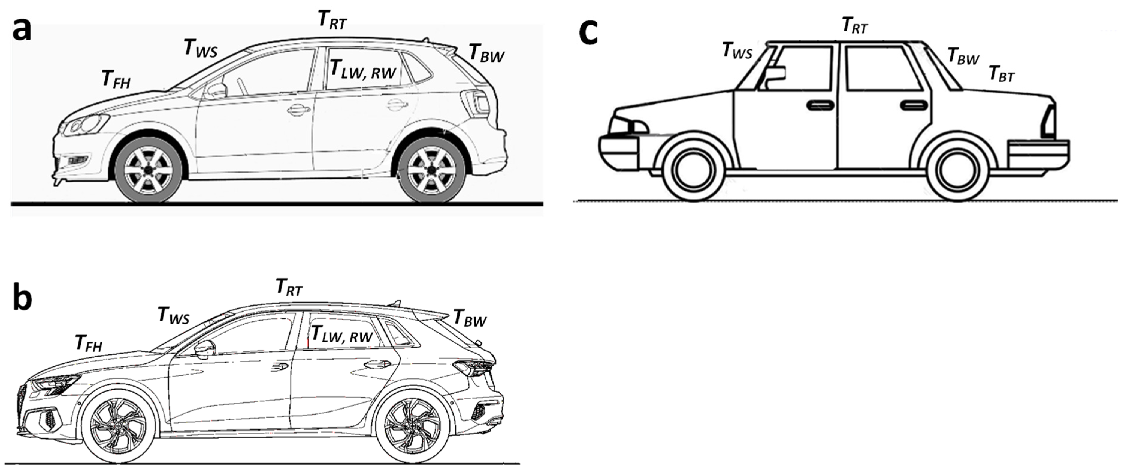
2.2. Characteristics of the Condensing Surfaces

The reference condenser was planar (0.5 m × 1 m). It was set horizontally on the ground. It was made of a specific condensing foil [17], thermally isolated underneath by 25 mm Styrofoam. This foil (of food quality) was made of a low density polyethylene film, 0.3 mm thick, in which a few % of TiO2 and BaSO4 microbeads were embedded, plus a food proof surfactant insoluble with water at its surface [18].
The car rooftops (Table 3 and Figure 4) were usually made of painted steel. The composition of steel was 0.08 to 0.18% C, 1.6 to 2.4% Mn, 0.4% Cr + Mo for cold-rolled steel. It was 0.05% C, 1% S, 1.5% Mn, 0.6% Cr, 0.4% Mo for hot-rolled steel and 0.14% C, 2.10% Mn, 0.40% Si for cold-rolled steel [19]. Steel thickness was in the order of 1.2 mm. Thermal isolation was usually present by an isolation material underneath. For instance, a thin layer of aluminum was attached to the roof trim of the car, and a hollow layer was set between the roof trim and the roof’s outer panel. However, the quality of the thermal isolation depends on the trademark, and we would rather consider it near-thermal isolation. Emissivity was paint emissivity, between 0.92–0.96 (Table 3).
Table 3. Some characteristics of different car surfaces compared to water properties (room temperature). (a) [20]. (b) [21]. (c) [22] (in the atmospheric window (7.5–14 µm)). (d) Low density polyethylene. (e) [17].
Car partMaterialsThickness (mm)Thermal Conductivity
(W·m−1·K−1)
Surface Emissivity
Rooftop RTpaintsteelisolation0.008–0.0381.2100.57–1.48 (b)54~0.030.92–0.96 (a)--
Front hood FH
Back trunk BT
paintsteelisolationnon isol.0.008–0.0380.7–2100.57–1.48 (b)54~0.030.92–0.96 (a)--
Windshield WSglassvinylglass2121.05 (a)0.25 (a)1.05 (a)0.92–0.94 (a)
Windows Wglass3–61.05 (a)0.92–0.94 (a)
Water (liquid)water-0.606 (a)0.98 (c)
Airair-0.026 (a)-
Reference REFfoilstyrofoamair0.325100.33 (a,d)0.032 (a)0.024 (a)0.90 (e)
Windshields are generally made of two pieces of glass about ew = 2 mm thick with an approximately ev = 1 mm layer of poly-vinyl butyral sandwiched in-between (Figure 4). Recently, many windshields included another thin, sound-absorbing vinyl layer to reduce road noise. Emissivity was that of glass (0.92–0.94 in the atmospheric window [7.5–14 µm], see Table 3). Other windows were made with tempered glass, 3–6 mm thick, whose properties are listed in Table 3. Table 4 summarizes the tilt angle φ for each studied surface according to the car model. The angles were in the trigonometric order (left side windows and windshield thus correspond to φ > 0 and right side and back windows to φ < 0).

2.3. Data Collection

2.3.1. Meteo Data

(i)
Ajaccio
A meteorological station (Froggit HE4000) was installed at 30 m NNW from the car. The station records classical meteorological parameters with a 1-minute time step: ambient air (Ta, °C), relative humidity (RH, %), dew point temperature (Td, °C), windspeed (V, m·s−1 at 2.5 m from the ground), wind direction (degrees), absolute pressure (hPa), and rain precipitation (mm). The measurements characteristics were the following: temperatures (−40 °C–60 °C, 0.1 °C resolution), relative humidity (10%–99%, 1% resolution), windspeed (0–50 m·s−1, 0.5 m·s−1 resolution, 0.3 m·s−1 stalling speed), wind direction (0–360°, bin-width 22.5°), and atmospheric pressure (300–1100 hPa, 0.1 hPa resolution), rainfall (0–9999 mm, 0.3 mm resolution).
Cloud cover data (in oktas) were computed from the sky conditions observations (“Fair,” “partly cloudy,” “cloudy,” etc.). Data were obtained from Météo-France, the French Meteorological Network (30-min time-step) installed at the Ajaccio airport (8°47′37″ E, 41°55′10″ N, 5 m asl). The measurement site was at 5.3 km from the airport in the SSW direction.
(ii)
Valparaiso
The weather station was a PCE-FWS 20 collecting classical meteorological parameters (Ta, Td, RH, direction, and windspeed at 1.7 m from the ground, atmospheric pressure, rain precipitation). It was located within 3 m from the vehicle under study in the E direction (see Figure 2b). The measurements characteristics were the following: temperatures (0–50 °C, 0.1 °C resolution), relative humidity (1–99%, 1% resolution), windspeed (0–50 m·s−1, 0.1 m·s−1 resolution, 0.3 m·s−1 stalling speed), wind direction (0–360°, bin-width 22.5°), and atmospheric pressure (300–1100 hPa, 0.1 hPa resolution), rainfall (0–9999 mm, 0.3 mm resolution). Cloud cover was observed in the evening and morning.

2.3.2. Surface Temperature Measurements

Figure 5 shows the location of the temperature sensors in the studied cars. More precisely:
(i)
Ajaccio
Cars were instrumented before night with 4 type K thermocouples (Figure 5a,b) and a data logger (TEKCOPLUS Ltd., type THTK-6, precision ± 0.1 K). Data were recorded with a 1-minute time step. The surface temperature (T0) of the reference planar condensing foil was also measured with a thermocouple connected to the data logger. Since only 4 temperature measurements were available together, nights were studied with always reference and air temperatures (the latter to compare with the meteo station data) and two variable car surfaces temperatures (e.g., RT and WS or RT and FH, etc.).
(ii)
Valparaiso
Temperature sensors (Thermochron iButton DS1922L, semiconductor temperature sensor) were used to measure temperatures in 18 locations. Each sensor stores data independently, with 4096 readings, 16-bits, 0.0625 °C resolution. Sensors were put on the outer part of the RT and FH surfaces and the inner part of the WS and BW surfaces (Figure 5c). In addition, a measurement was made on the inner part of the RT thermal isolation. Other surface measurements were performed; they are not discussed here.

2.3.3. Dew Volume Measurements and Observation Protocol

(i)
Ajaccio
Visual observation of the car was carried out in the morning before sunrise according to the method described in the Introduction and Equation (1). The collection of dew on each surface of the car is difficult due to the configuration of the surfaces (curvatures, accessibility), the condensed volumes were thus collected on the selected surface by pressing during a few s a spongy tissue (0.35 × 0.5 m², 2.5 ± 0.5 mm thick). Since on inclined surfaces the drops slide down during the night, the collected volume on such surfaces will be less than the actual condensed volume. These data were thus not reported for the window surfaces.
Concerning the horizontal reference substrate (foil), water droplets were collected in a bottle by scraping. Water was always collected in the morning before sunrise and immediately weighted (electronic balance, resolution 0.1 g, precision ± 0.1 g).
(ii)
Valparaiso
Observation at sunset was made of dew on RT, FH, and BT, side windows, corresponding to the visual scale n = 3. There was no dew volume measured.

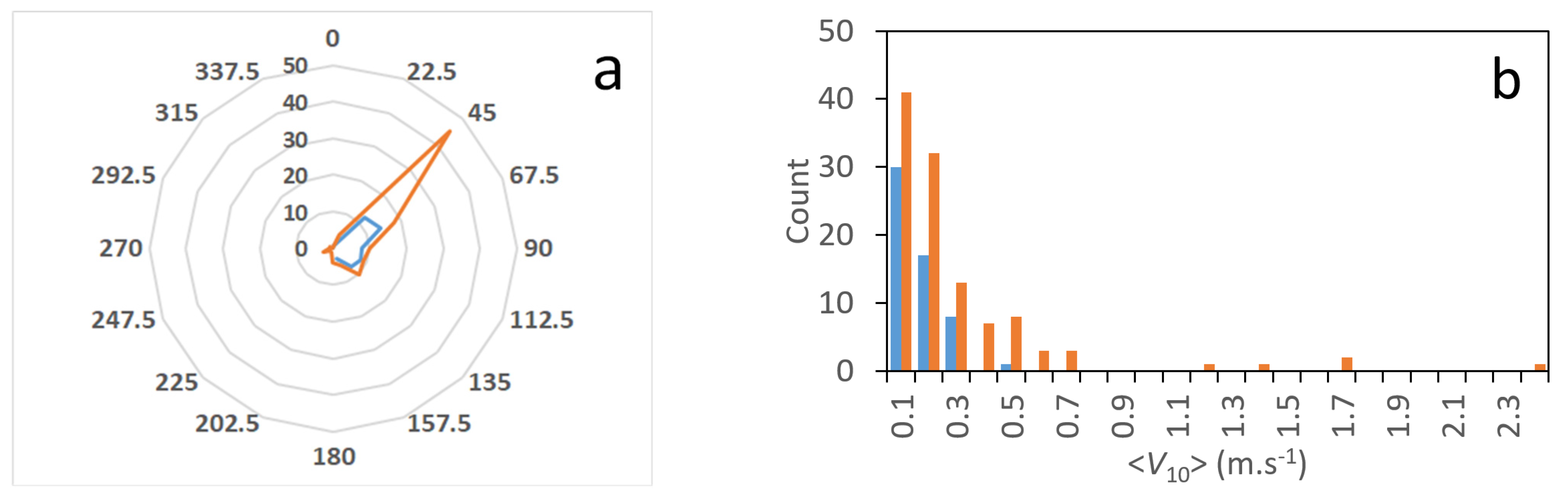
2.3.4. Wind Velocity Extrapolation at 10 m Elevation

Windspeeds V as measured at 2.5 m above the ground (Ajaccio) and 1.7 m (Valparaiso) were extrapolated at the standard value V10 extrapolated at 10 m by using the classical logarithmic dependence of air flow above the ground. The corresponding function to describe the wind profile V(z) [23], where z is the height measurement above the ground, is expressed as:
V ( z ) = V 10 ln ( Z z c ) ln ( 10 z c )
Here zc is the roughness length (taken to be zc ≈ 0.1 m). It corresponds to (Ajaccio) V10 = 1.43 V2.5 and (Valparaiso) V10 = 1.62 V1.7.

2.3.5. Relative Temperature Efficiency

The temperature decreases T j of a given car external surface j (e.g., j = RT) with respect to air temperature Ta is compared with the corresponding quantity relative to the surface temperature T0 of the horizontal reference condenser according to the ratio
Δ T j * = T j T a T 0 T a
This temperature efficiency was already defined in previous works [16,24]. Means are considered only during the condensation period, that is, with T d the air dew point temperature, when:
T j T d < 0
The Δ T j * values for surface j are computed every minute during the night. These values are filtered following Equation (6), then averaged to obtain a nightly value. To have a mean value over time, the nightly values of Δ T j * are averaged for all considered nights (with standard deviation). The mean values Δ T j * ¯ over p measurements are calculated as
Δ T j * ¯ = 1 p i = 1 p Δ T j , i *

3. Dew Yield, Surface Temperature, and Radiation Deficit

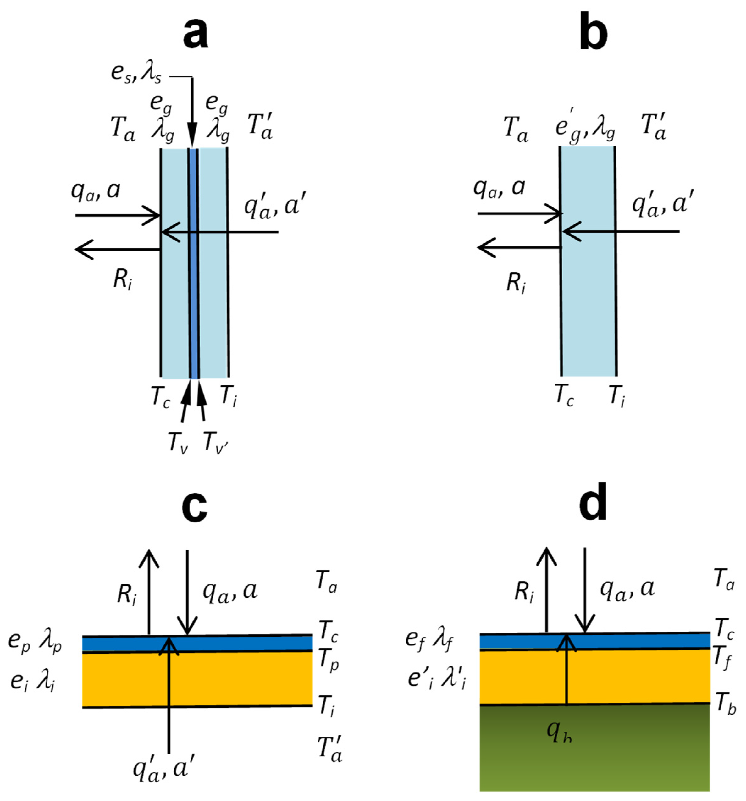
3.1. Radiative Cooling

Dew condensation is ensured by radiation cooling. The radiation deficit Ri of a body at temperature Tc when exposed to clear sky radiation at temperature Ta can be expressed by the Stefan–Boltzmann law. Denoting εc the condensation surface emissivity and εs the nocturnal clear sky emissivity averaged on scattering angles and radiation wavelength (see below Section 3.2), one obtains, with σ the Stefan-Boltzmann constant:
R i = ε c ε s σ T a 4 ε c σ T c 4 = ε c σ ( ε s T a 4 T c 4 )
The first term corresponds to the radiative power absorbed from the atmosphere and the second term is the power emitted by the condensing surface. Neglecting the small temperature difference between the condensing substrate temperature (Tc) and ambient air (Ta) when expressed in K, Equation (8) becomes:
R i ε c σ ( 1 ε s ) T a 4 σ ( 1 ε s ) T a 4
Since the emissivities of dry and wet car surfaces are close to unity (Table 3), we thus consider for simplicity in the above Equation (9) the surfaces to be perfect black bodies with emissivity ε c = 1. This is not far from the actual emissivity as wet surfaces emissivities are always close to water emissivity 0.98 [25]. The radiation deficit is in general negative because ε s < 1 .
Clear nocturnal sky emissivity, εs, averaged on scattering angles (see below Section 3.2) and radiation wavelength, depends strongly on the atmosphere water content. In particular, it exhibits a near-linear relationship with air dew point temperature Td near the ground surface [26]. The following estimation [8] takes into account the atmosphere water content and the site elevation H (km) from [27] and also the cloud cover expressed in fraction c of the cloudy sky. With Td in °C:
1 ε s = [ 0.24221 + 0.204323 H 0.0238893 H 2 ( 18.0132 1.04963 H + 0.21891 H 2 ) × 10 3 T d ] ( 1 c ) )
The radiation deficit is thus a function of Ta and Td (from εs) or, equivalently, of Ta and air relative humidity RH near the ground. One notes that air should be humid enough to permit condensation within a few degrees below the air temperature (see Section 4.3.2), but this humidity limits, in turn, the available cooling energy by increasing the sky emissivity.

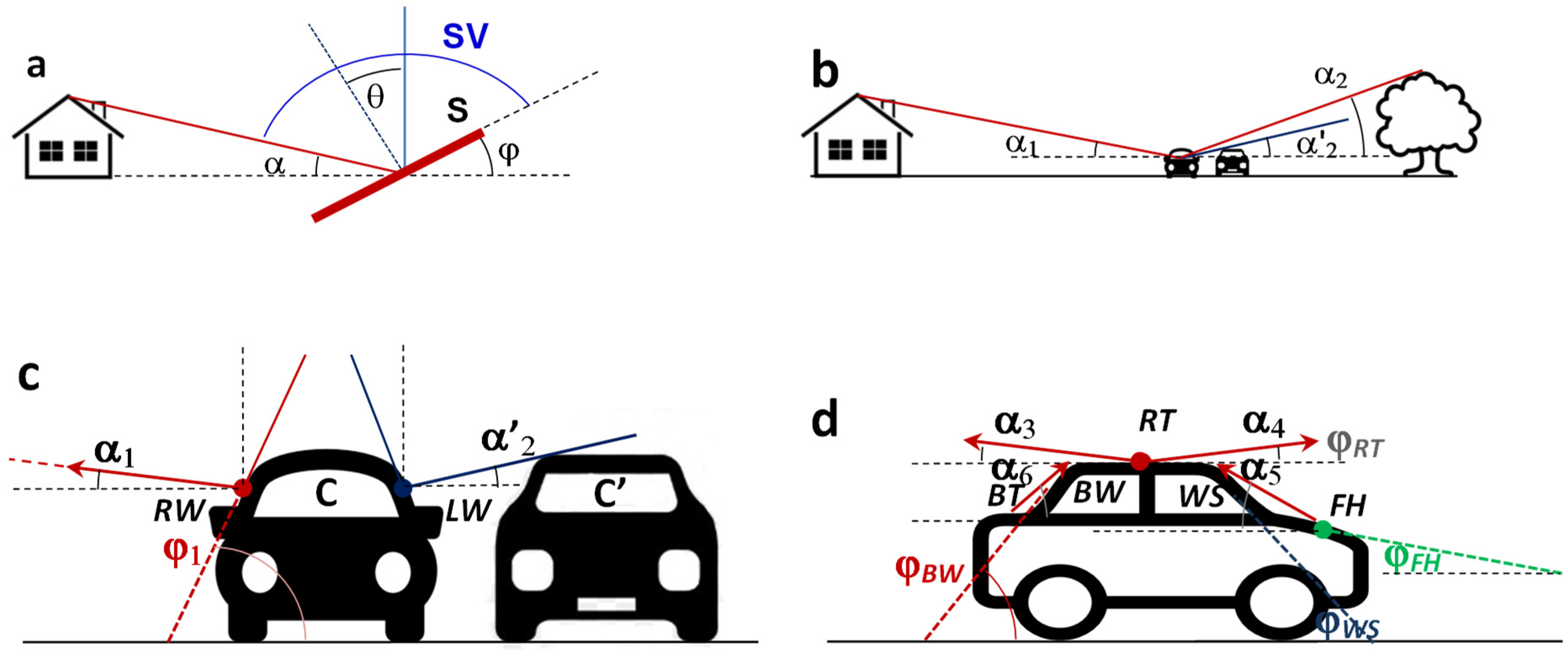
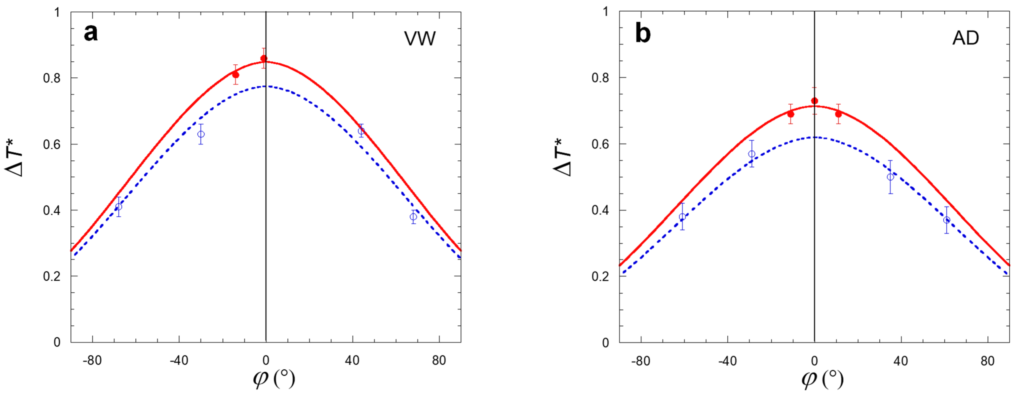
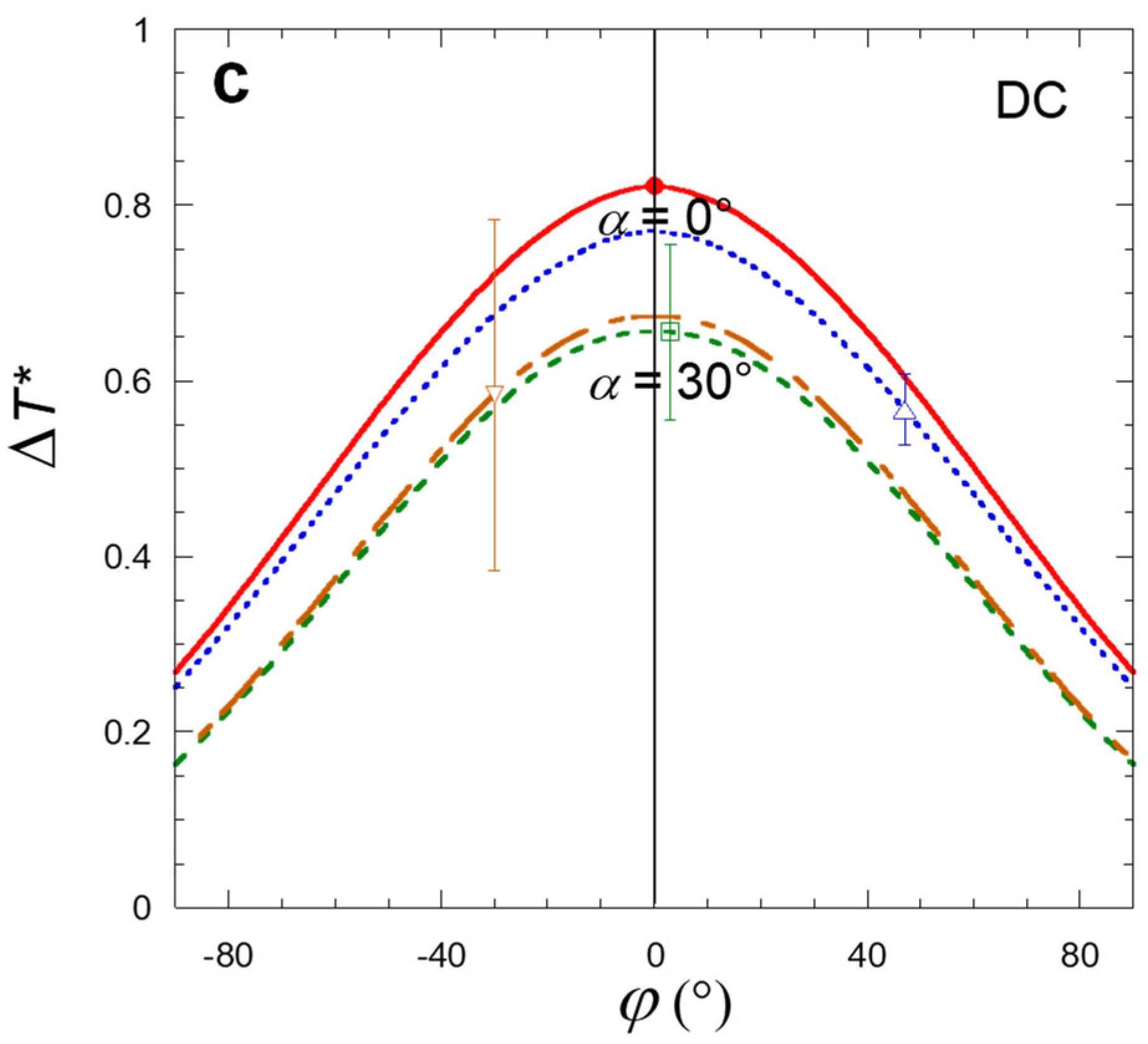
3.2. Radiative Heat Exchange with Surface Tilt Angle and Obstacle View Angle

The main parameters, which affect the radiative deficit are the angular dependence of the sky (atmosphere) emissivity, the inclination of the substrate with horizontal and the angle of views of obstacles emitting IR radiation around (trees, buildings, nearby cars, see Table 2).
Concerning the sky emissivity, its angular dependence can be evaluated as a function of total emissivity ε s [28,29]. With θ the angle with vertical:
ε θ = 1 ( 1 ε s ) 1 b cos θ
Here b = 1.8 is a numerical constant [26]. The vertical ( θ = 0°) emissivity ε 0 λ can be related to the total emissivity by ε 0 = 1 ( 1 ε s ) 1 b , from which one infers a relation between vertical or total and angular spectral emissivities:
ε θ = 1 ( 1 ε 0 ) 1 cos θ
The directional spectral emissivities can be computed from Equation (11) (Figure 6a) with respect to θ for different total spectral emissivities ε s . One notes that the emissivity in directions near the vertical θ ≈ 0–20°) was almost constant with respect to θ . Near horizontal emissivity θ ≈ 80–90°) always reaches unity. With total angular emissivity for a typical night of about ε s ≈ 0.84 (Equation (10)), it corresponds (Figure 6a) to an angular emissivity varying between 0.72 ( θ = 0°) and unity ( θ = 90°).
The radiative cooling limiting factor was the sky view and the IR emissions of nearby obstacles, both factors that depend on the surface tilt angle. Table 2 reported the largest available sky view corresponding to each surface together with the tilt angles. In Figure 6a, the schematics of limiting sky views were reported. The regions outside the sky view have an emissivity close to unity and will heat up the condensing surfaces. However, when the angles α and φ were lower than ~20°, which was the case in this study except for the side windows, their effect will be about the same as from the lower layers of the atmosphere (assuming they are at the same temperature) and could be neglected. This is corroborated by the study of the influence of the tilt angle φ and obstacle view angle α on the radiative deficit of a plane surface [30]. In Figure 6b is shown the surface tilt angle dependence of the radiative deficit for Ajaccio with air temperature Ta = 15 °C by interpolating the Howell et al. data [30]. The mean value measured on a horizontal substrate in Ajaccio was 88.9 W·m−2 [31]; it corresponds in the Howell et al. data [30] to a low path-integrated precipitable water vapor PWV = 0.78 cm. Figure 6c shows the relative variation of the reduced radiation deficit R i ( α ,   φ ) / R i ( 0 , 0 ) with respect to the tilt angle φ at different sky view angles α . The data corroborate and precise the discussion concerning Figure 6a: the influence of the tilt angle becomes negligible for φ < 30° and α < 15°.

3.3. Energy Balance

The balance of energy at the droplet condensing surface can be written by considering the radiative cooling heat flux Ri (<0), the convective heat flux from the air outside the car, qa and heat flux from inside the car, qi, and the release of latent heat during condensation, qc. For simplification, the thermal resistance of droplets was neglected due to their small size (<mm). Since nearly all condensation process was made during the time period where drop grows by diffusion and coalescence, one will consider an equivalent film with thickness h (see, e.g., [32] and refs. therein; [6]). All fluxes were per unit surface area.
It follows the equation, during the steady state where the condensing surface temperature Tc does not vary with time t ( d T c / d t = 0 ):
R i + q a + q i + q c = 0
Since q i corresponds to warming from inside air, one can define a mean warming heat flux q a , j * from the air for surface j and mean heat transfer coefficient a j for surface j. It happens that q a , j * can be expressed as a function of TaTj (see Section 3.4 below) such that a mean heat transfer coefficient a j can be defined:
q a , j * = q a , j + q i , j = a j ( T a T j )
Writing Lv the latent heat of condensation, m the condensed mass, v the corresponding volume, Sc the condensing surface area and h = v / S c , the condensed volume per surface area, the condensation heat flux can be written as
q c = L v 1 S c d m d t = ρ w L v h ˙
where ρ w is liquid water volumic mass and h ˙ d h / d t is the condensed volume per surface area. The evaluation of fluxes q a and q i is made in the following Section 3.4.

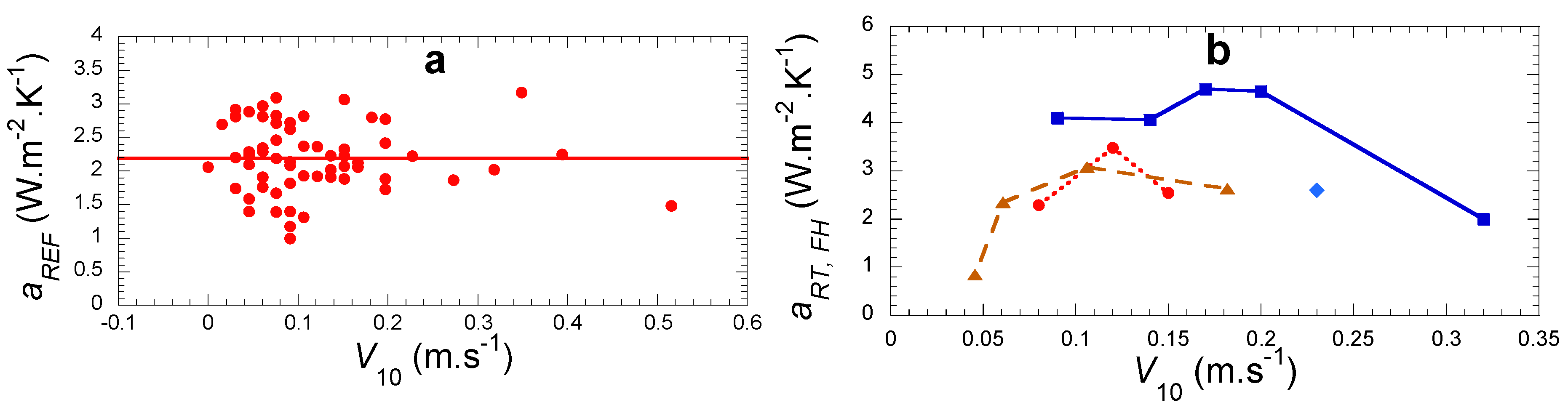
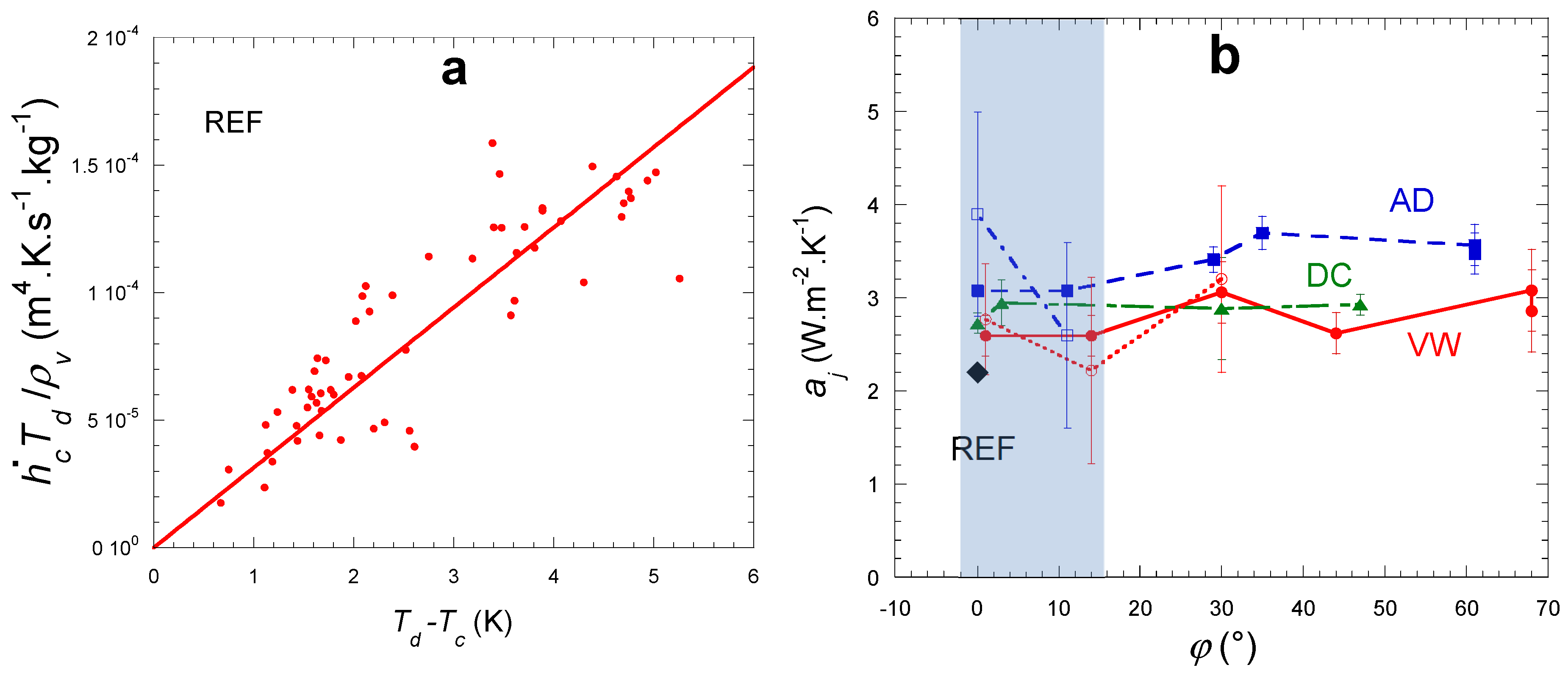
3.4. Conductive and Convective Heat Exchange

All surfaces exchange heat with air, inside and outside the car. The thermal heat exchange depends on whether air flow is made by natural convection or due to forced air flow.
For surfaces inside the car, convection is natural, and air flow is parallel to the surface. Surfaces outside the car can be either submitted to natural convection when windspeed is small or forced convection if not. Experiments [33] and simulations [34] show that the typical natural convection velocity is on the order of V0 = 0.6 m·s−1. This means that three situations can be met: single natural convection V << V0, forced air flow for V >> V0, and mixed natural-forced convection for VV0. Natural convection corresponds to the situation inside the car. Since the data obtained in this study correspond to relatively small windspeeds, lower than a few m· s−1, one will make in the following the simplifying assumption that the heat exchange coefficient a with air is the same inside the car (natural convection) and outside (mixed natural and forced convection). The study of the heat transfer coefficients with windspeed and wind direction (Section 4.2.2) confirms this assumption. The corresponding heat fluxes q a (outside the car) and q a (inside the car) can thus be written as:
q a = a ( T a T j )
q a = a ( T a T j )
where temperature T j is inside temperature of the j-surface and T j is the outside temperature. Heat exchange with air strongly depends on air flow configuration above the condensing surface, as seen in CFD simulations [34,35,36]. Typical values were 5–8 W·m2·K−1 for natural air convection and 20–30 W·m2·K−1 for forced air convection [37]. For a horizontal plane, a calculation concerning natural convection triggered by a temperature difference T a T j ≈ 5 K gives a hydrodynamic boundary layer thickness δ H on the order of the thermal boundary layer δ T 1.3   δ H 2.6 mm [6]. It follows the heat transfer coefficient
a = λ a δ T
with λ a   = 0.026 W·m−1·K−1 (see Table 3), one obtains a = 10 W·m2·K−1. When forced convection is concerned on a plane, the hydrodynamic boundary layer thickness under laminar flow is classically expressed by δ H = 5 ( ν x / U ) 1 / 2 [38,39] with x the distance from the edge of the plane, U the incoming air flow velocity, and ν (≈ 14 × 10−6 m2·s−1; [20]) the air kinematic viscosity. For typical values x = 1 m and U = 1 m·s−1, the thermal boundary layer δ T 1.3   δ H 20 mm. It follows the heat transfer coefficient from Equation (18), a = 1.3 W·m2·K−1. One will see in the following that the values were not exactly the expected values because (i) the actual air flow was most often a mix-up of natural and forced flow configuration, and (ii) the flow was rather turbulent due to the influence of edges. For an open planar structure, turbulence is expected to occur for a Reynolds number Re =   U x / ν > 5 × 10⁵ [40]. Turbulence should then occur for U > 7 m·s1 with x = 1 m, meaning that most winds giving dew (U < 4.4 m·s−1, see [8]) should correspond to laminar flows. However, when obstacles and edges were present, which is always the case, turbulence was known to occur at much smaller values of Re. Practically, although the assumption of laminar flow was simplifying as it leads to analytical formulae, the air flow under actual conditions was most likely to be turbulent. As a matter of fact, the experimental results discussed in Section 4.2.2 can only be understood if turbulence is present.
Another way of calculation is concerned with energy balance. Dew does not form on planar condensers thermally isolated underneath when T a T c > Δ T 0 ~ 15 K [6]. Typical radiative deficit values in humid air is R i ≈ 60 W·m−2 [26]. It corresponds in Equation (13) to have q i = q c = 0 , and then allows a to be estimated as a = R i / Δ T 0 . It thus follows a value a ~4 W·m−2·K−1. On the other hand, from [8] (see also Section 4.3.2), where is also used an energy balance approach, one can deduce a mean value a ~ 3.5 W·m−2·K−1, in agreement with the above value. In Section 4.3.1, one estimates the heat transfer coefficient on the REF plane to be a = 2.2 W·m−2·K−1. This latter value will be used in the following when necessary.
Concerning the rooftop, the heat flux from inside the car (Figure 4c) can be written, with notations from Figure 4:
q i , R T = ( 1 e p λ p + e i λ i + 1 a ) ( T a T R T )
When considering the numerical values of Table 3, one can neglect the metal conduction contribution e p / λ p with respect to air contribution 1/a. During dew condensation, inside air, cooled by the external car surfaces, is in general colder than air outside (Figure 7). A rough approximation for evaluating its temperature is taking T a ~ ( T R T + T a ) / 2 , which allows q i , R T to be expressed in the simple form:
q i , R T ~ 1 2 ( 1 e i λ i + 1 a ) ( T a T R T ) = 0.63 ( T a T R T )
With T a T R T < 5 K, the warming heat flux q i , R T corresponds to a heat flux of less than 3.2 W·m−2. From Equation (14) and using the numerical values from Table 3, one obtains the mean heat transfer coefficient a R T   = 2.2 + 0.63 = 2.83 W·m−2·K−1, that is, an increase of about 28% with respect to a fully isolated horizontal surface such as the REF surface. From Table 5, where the ratio of heat transfer coefficients of car parts are listed with respect to the reference surface as determined in Section 4.2.1, one can see that the measurements are in relatively good agreement with the above calculation.
Concerning the side and back windows (Figure 4b), the heat flux from inside the car can be written, with λ g and e g the glass thermal conductivity and thickness, respectively:
q i , W = ( 1 e g λ g + 1 a ) ( T a T W )
Table 3 data show that one can neglect e g / λ g with respect to 1/a. Equation (21) then becomes:
q i , W a ( T a T W )
The same kind of calculation leads, for windshield (Figure 4a), to
q i , W S = ( 1 2 e g λ g + e v λ v + 1 a ) ( T a T W S ) a ( T a T W S )
Here eg is glass thickness and λ v and ev are the vinyl film thermal conductivity and thickness, respectively. It thus follows that both W and WS exhibit the same warming fluxes.
Let us consider now the same rough approximation for evaluating window temperatures as performed for RT, T a ~ ( T W , W S + T a ) / 2 . Equation (23) becomes:
q i , W S = q i , W = a ( T a T W S )
From Equation (14) and using the Table 3 numerical values, one expects, with T a T W S < 3K, a heat flux lower than 7 W·m−2. It corresponds to a mean heat transfer coefficient a W , W S = 3a/2, that is an increase of 50% with respect to a fully isolated horizontal surface such as the REF surface. This is in agreement with the Table 5 values in Section 3.2 where, in addition, the W and WS heat transfer coefficients are found to be close together, as expected. One notes that the AD car heat exchange coefficients are systematically larger than those of the VW car. One attributes this increase to enhanced air flows due to a different car geometry.
The inner temperature of the car, T a , was recorded in Ajaccio (VW car) and Valparaiso (DC car), see Figure 7. It approximately follows the rooftop and window temperatures. The shift of temperature is ( T R T T a ' ) ≈ −5 K (VW car) or −3 K (DC car). With a~2.2 W·m−2·K−1, the corresponding heat flux from inside air to non-isolated surfaces (e.g., windows) is thus nearly constant and on order 3–7 W·m−2 from Equations (19) and (23). This flux corresponds to a cooling flux for inside air temperature; it explains its evolution during the night, parallel to rooftop and window temperatures evolutions.
One notes that the thermal resistance is negligible for the glass windshield and the metallic part of the roof top and front hood. It thus means that the inner and outer surface temperatures are the same for those surfaces.
Let us now consider the reference condenser set on the ground whose temperature is Tb (Figure 4d). The ground surface temperature is unknown, but it should be somewhat less than the air temperature. In addition, the contact foil-Styrofoam and Styrofoam-ground is loose. For reasons of simplification, one will then neglect the heat losses through the Styrofoam.

3.5. Relation Dew Yield—Surface Temperature

The condensation term in Equation (13) can be expressed from the difference in vapor pressure from ambient air, p v ( T a ) , and saturation pressure at Tc, p s ( T c ) . With aw the mass diffusion coefficient of water molecules in the air,
d m d t = a w S c [ p v ( T a ) p s ( T c ) ] = a w S c [ p s ( T d ) p s ( T c ) ]
The water vapor transfer coefficient aw is proportional to the heat transfer coefficient a. They indeed both correspond to diffusive processes through a gradient (water molecules concentration or temperature) in boundary layers of nearly the same extent, the values of the thermal diffusivity coefficient and the diffusion coefficient of water molecules in air being close (DT = 2.3 × 10⁻⁵ m2·s−1 and D = 2.3 × 10⁻⁵ m2·s−1). With γ (≈65.5 Pa·K−1) the psychrometer constant, one obtains (see, e.g., [6]):
a w = 1 γ L v a
In order to make apparent a heat transfer coefficient, one can express Equation (26) in terms of temperature difference from the Clausius-Clapeyron relation (see, e.g., [41]). With ρ v the water vapor volumic mass
p s ( T d ) p s ( T c ) ρ v L v T d ( T d T c )
Equation (27) thus becomes, in units of volume per condensing area ( h ˙ c d h c / d t ):
h ˙ c = a ρ v γ T d ρ w ( T d T c )
When T c is not measured (in contrast to the present study, see Section 4.3.1), one needs to obtain h ˙ c to determine T c . This is performed by numerically solving Equations (13) and (28) by iteration [42]. An alternative is to evaluate the heat losses in Equation (13) by an approximated evaluation where one assumes T c T a T d T a as performed by [8] and in Section 4.3.2.

3.6. Relation Temperature Efficiency—Radiation Deficit

The condensation term in Equation (13) is in general negligible with respect to the heat losses. For instance, for a typical dew rate 0.01 mm.h−1, it corresponds to a 7 × 10⁻³ W·m−2 power while with a typical cooling TaTc~5K and a heat transfer coefficient 2.2 W·m−2 K−1, heat losses are 11 W·m−2). Equation (13) thus becomes, with a j the heat transfer coefficient of the j-surface:
R i ( α , φ ) + a j ( T a T j ) = 0
One can express the heat transfer coefficients by comparison with the reference foil value to remove the influence of the radiation deficit. The temperature yield can then be written as:
Δ T j * ( φ ) = ( a 0 a j ) F α ( φ )
with
F α ( φ ) = [ R i ( α , φ ) R i ( 0 , 0 ) ]
The Figure 6c data, which represents the radiation deficit in Ajaccio with respect to φ can be fitted to a polynomial function of order 3 in φ (°):
α = 0 °
F 0 ( φ ) = ( 89.037 0.032145 | φ | 0.013164 φ 2 + 6.7921 × 10 5 | φ | 3   ) / 89.037
α = 15 °
F 15 ( φ ) = ( 87.841 0.040067 | φ | 0.013438 φ 2 + 7.1463 × 10 5 | φ | 3 ) /   89.037
α = 30 °
F 30 ( φ ) = ( 76.701 + 0.043085 | φ | 0.015329 φ 2 + 8.606 × 10 5 | φ | 3 ) /   89.037
α = 45 °
F 45 ( φ ) = ( 54.412 + 0.088672 | φ | 0.013183 φ 2 + 7.3988 × 10 5 | φ | 3 ) /   89.037

4. Results. Discussion
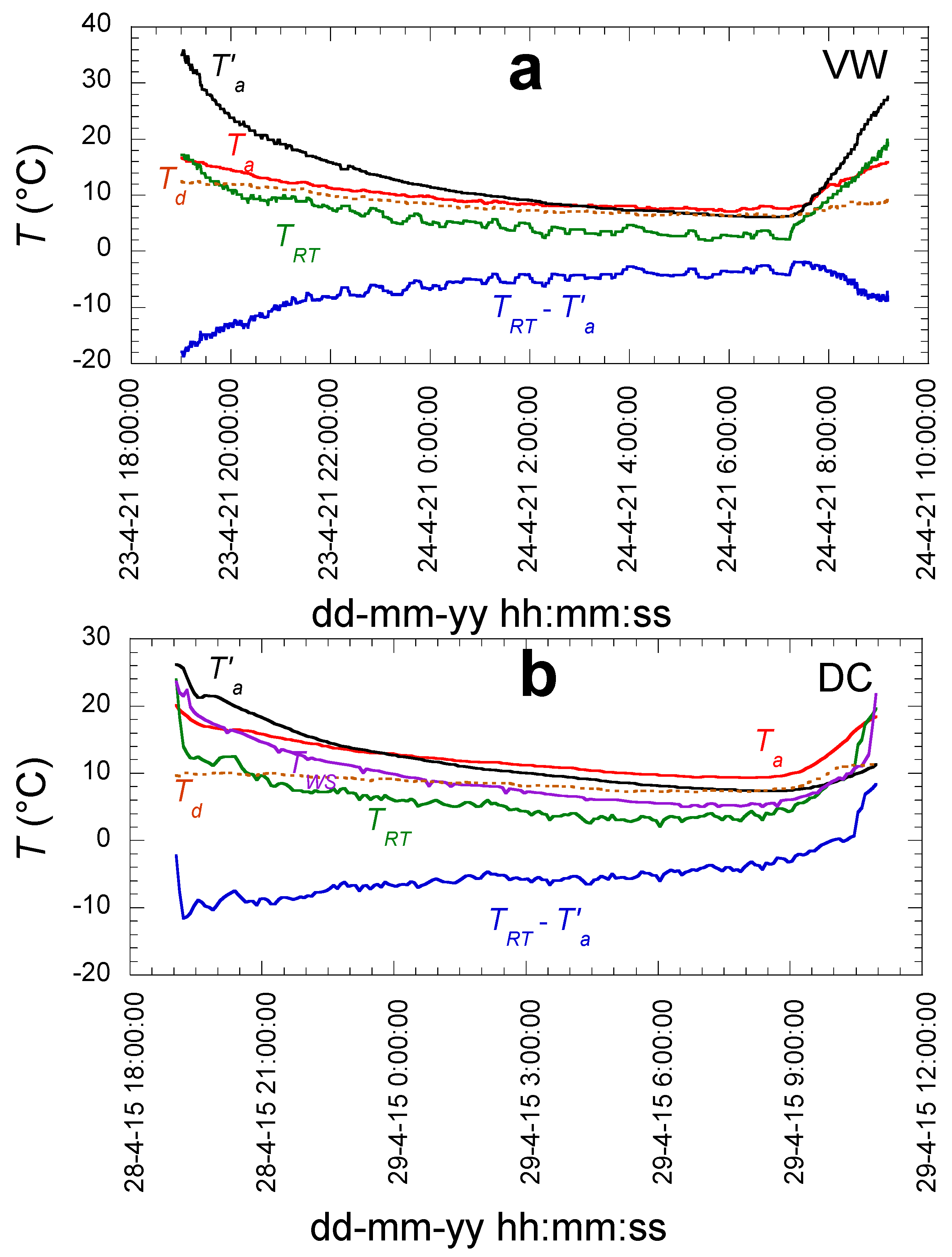
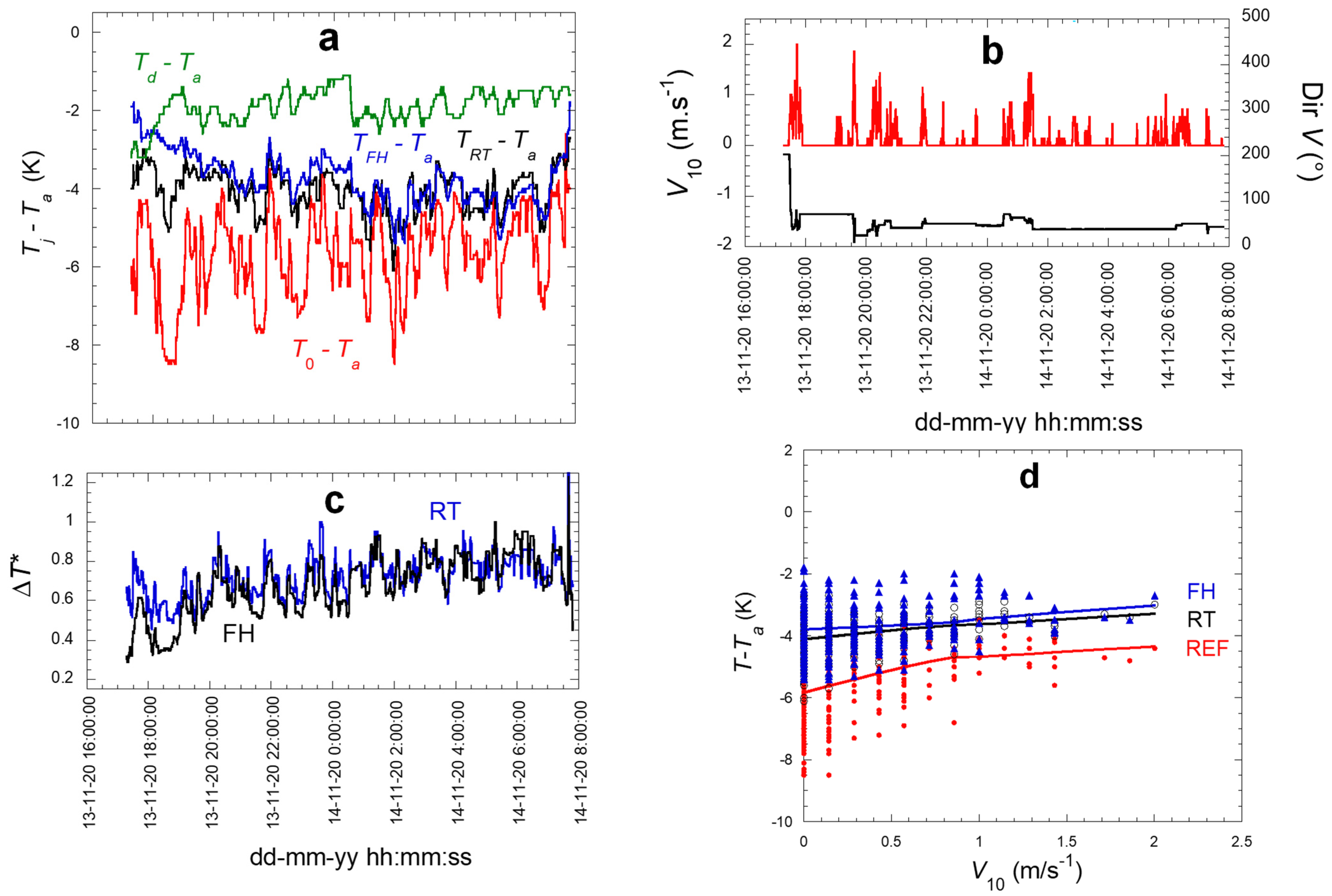
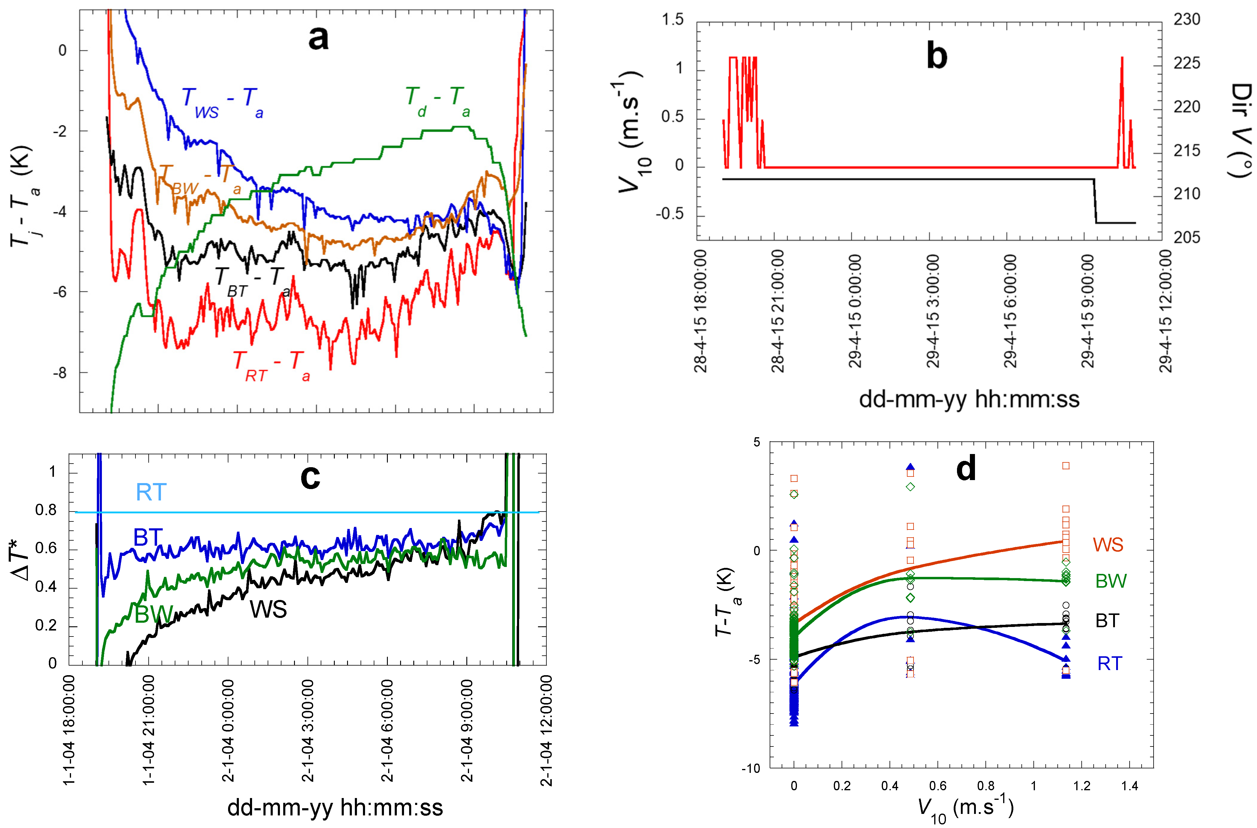
4.1. Typical Events

Typical nocturnal records measured on three cars are presented in Figure 8, Figure 9 and Figure 10. Due to the progressive cooling of the air inside the car, the windows temperatures reached a plateau only in the middle of the night, as shown by the cooling efficiency ratio Δ T L W ,   R W * (Figure 8c, Figure 9c and Figure 10c). When the cooling temperatures ( T j T a ) are plotted as a function of windspeed V (extrapolated at 10 m from the ground, Figure 8d, Figure 9d and Figure 10d), only a weak variation is observed on the near-horizontal surfaces. Note that, in Valparaiso (Figure 10d), the weakness of the windspeed does not allow clear trends to be observed. In Ajaccio, both left and right windows are preserved from the more frequent NE wind by the car itself (right side) or the neighboring car parked on the left (left side). The wind screen effect is weaker or not present for the horizontal surfaces (REF, RT, FH), whose temperature exhibits a weak but clear increase with windspeed (Figure 9d).
One sees in Figure 8a that during the night, left and right window temperatures were close together. Figure 8c presents a cooling efficiency for RW and LW nearly constant (mean value Δ T R W * = 0.37 ±   0.10). Note that, as already discussed, TRW and TLW were much less sensitive to windspeed than T0 (Figure 8d) because they are protected from the most common wind. This is corroborated by the temperature behavior of TRT and TFH in Figure 9d, which, with only partial screening from the wind (FH), exhibits a low increase with windspeed.
It is interesting to note that the temperature differences TcTa for car and reference surfaces do not vary much during condensation (Tc < Td). The temperature efficiency Δ T * is thus also nearly constant during condensation.

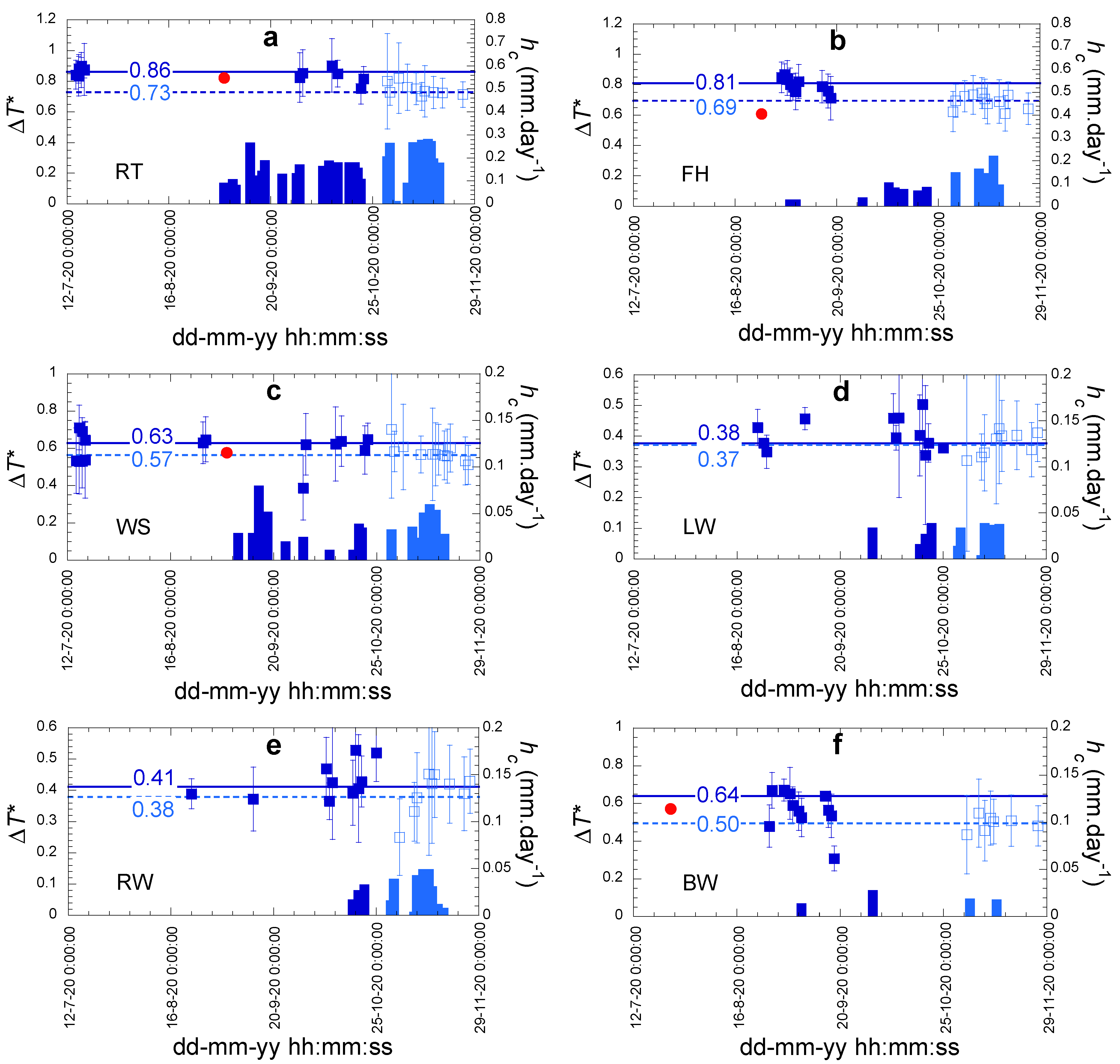
4.2. Temperature Efficiency and Dew Yield Evolution

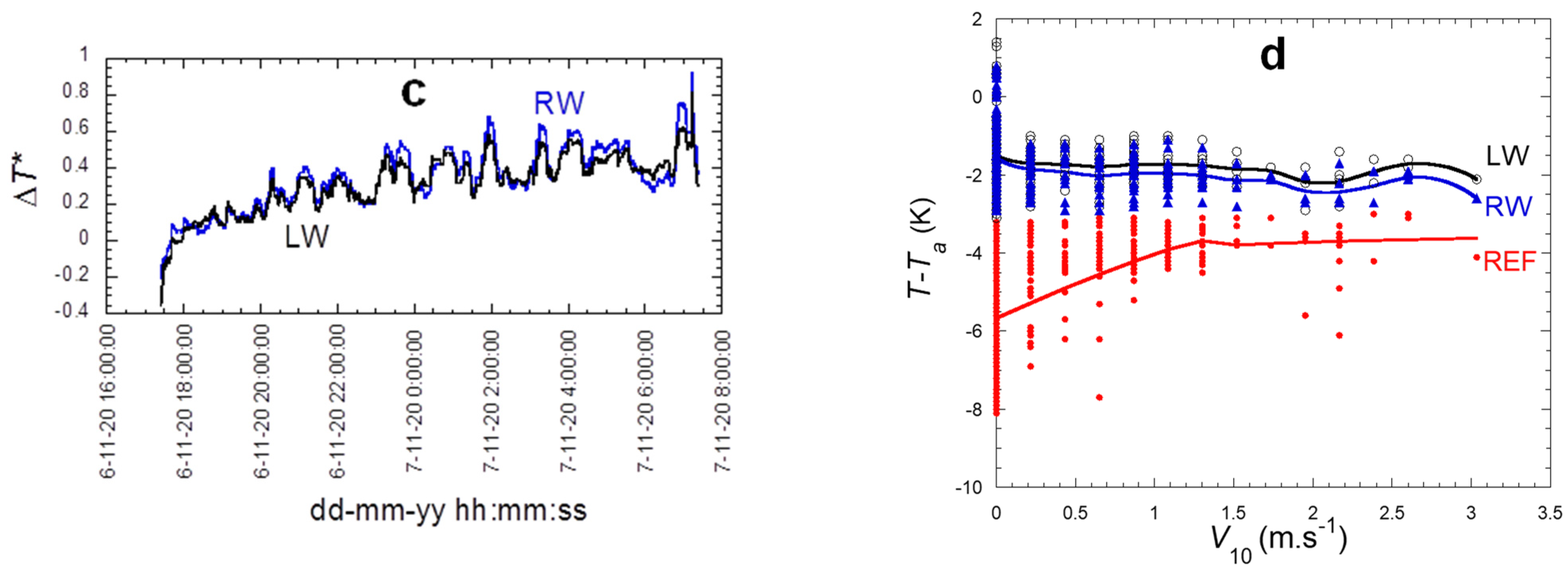
4.2.1. Temperature Efficiency

Daily mean cooling efficiencies Δ T * (Equation (5)) were calculated from the temperature data recorded in Ajaccio (Figure 11) from 15 July to 25 October 2020 (VW) and from 29 October to 30 November 2020 (AD). (Only one night, indicated by a red dot, is available in Valparaiso). A remarkable result is the constancy of ΔT* during the whole period, the only (weak) variation being due to a change of car model. The average Δ T * ¯ of all calculated values is reported in Table 5. One can observe that Δ T * ¯ < 1 for all surfaces in the following order (data from Valparaiso are included): 1 > Δ T R T * >   Δ T F H * > Δ T B T * >   Δ T W S * > Δ T B W * > Δ T R W * ~   Δ T L W * (Figure 11 and Table 5).
One can distinguish two main classes depending on whether the surface is isolated (RT, FH) or not (BT, WS, LW, RW, BW). Within a class, the surface tilt angle, φ, and the obstacle angle of view, α, also matter, as discussed in Section 3.2. Some approximations can be made for the obstacle’s view angles since the radiative deficit is nearly the same for view angles below 15° (see Figure 6c). In Table 4 are listed the corresponding approximations by using the values listed in Table 2. The Ajaccio site data will be then compared with all view angles α ≈ 0°, and the Valparaiso data will be concerned with both 0° view angles and a mean taken to be 30° concerning obstacles whose views vary between 0° and 45°.
To be more quantitative, one considers in Figure 12 the angular variation Δ T * ( φ ) (Equations (30–35)) from the angular variation of Ri for the mean Ajaccio and Valparaiso radiative deficits (Figure 6b,c and Equations (11) and (12)). The results of the fits of the Δ T j * ¯ data to Equation (32) (α = 0°: VW and AD cars in Ajaccio, RT and BT of the DC car in Valparaiso) and Equation (34) (α = 30°: BW and WS of DC car in Valparaiso), with only the ratio a j / a 0 left free, are reported in Table 5. Only two classes of coefficients were considered, corresponding to isolated or non-isolated surfaces. Note that considering the mean of Δ T j * over all nights was justified by the near windspeed independence of T j T a (see Section 4.1 and Section 4.2.2).
One first observe in Figure 12 that the angle variation follows the radiation deficit variation, which means that it is indeed the main factor determining the condensing abilities of tilted surfaces. The other factor is the heat exchange coefficient, which, for near-isolated, near-horizontal surfaces, RT and FH (VW, AD cars) exhibit heat exchange coefficients about 25% larger than for the foil reference surface. An enhancement of heat transfer of about 28% was indeed predicted in Section 3.4. Non-isolated surfaces (windows and back trunk) unsurprisingly exhibit still larger heat transfer coefficient, on order 40% larger than the reference. In Section 3.4, an increase in the order of 50% was expected. The variation of the heat transfer coefficients with tilt angle φ was ignored in this calculation, which means that it can be indeed neglected.
Note that the relative cooling efficiencies of the AD car were systematically smaller than those of the VW car. This decrease is very presumably the result of enhanced air flows due to a different car geometry that enhance the AD heat exchange coefficient, as already noted in Section 3.4 and Table 5.

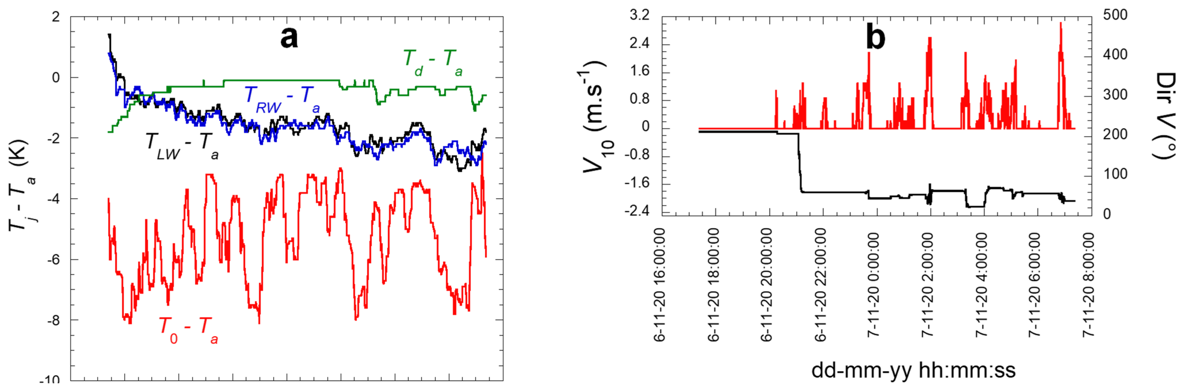
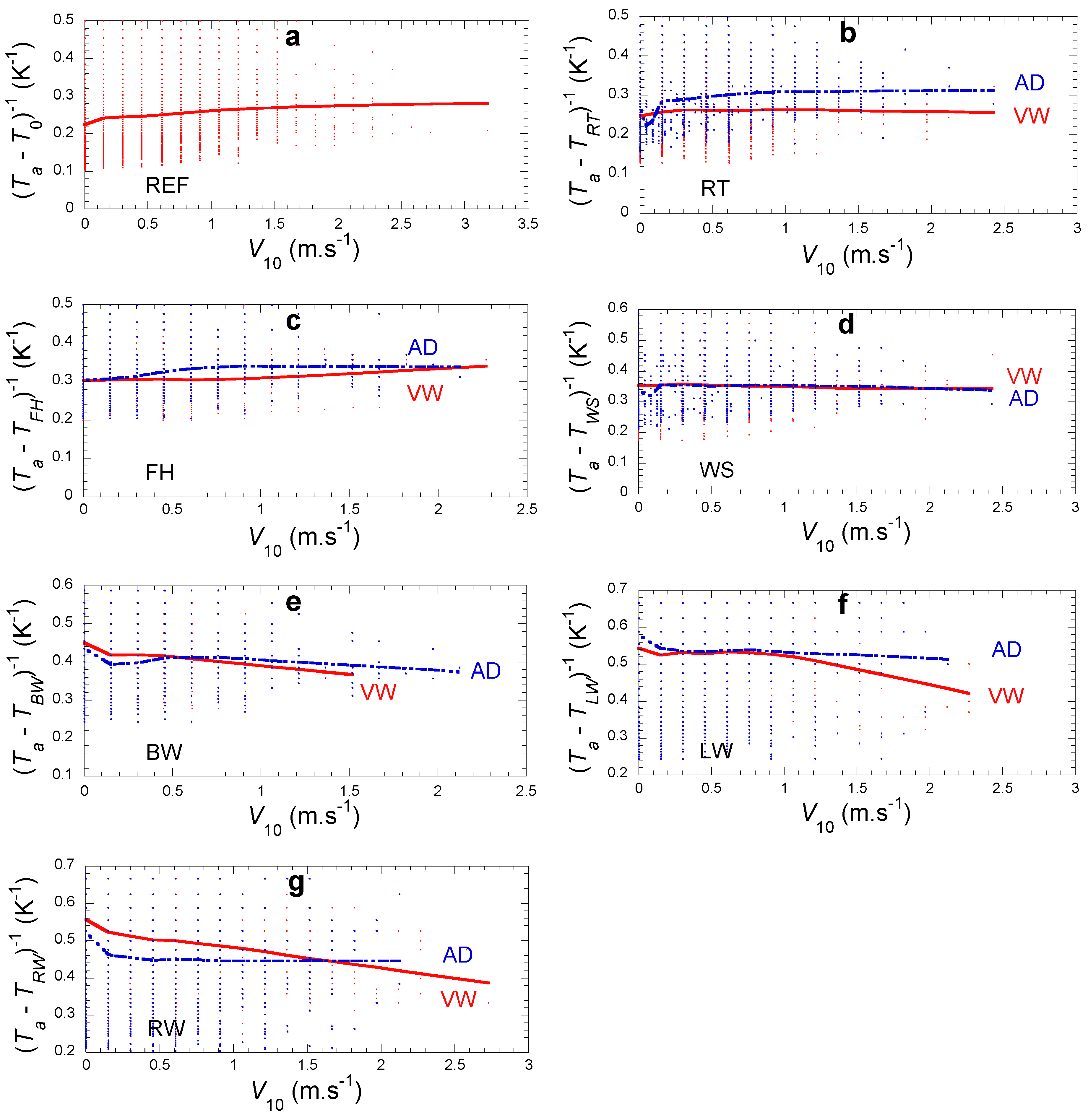
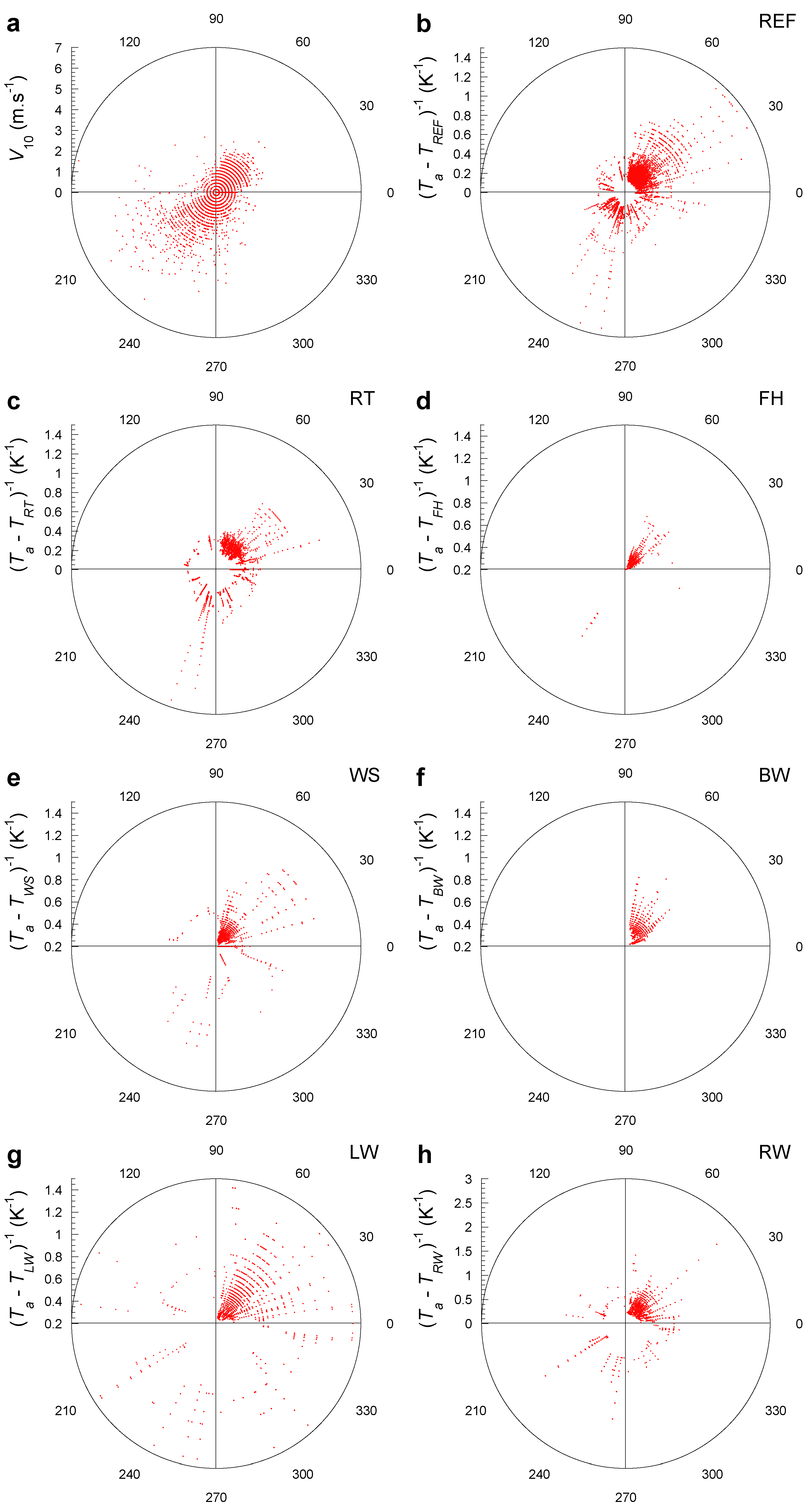
4.2.2. Surface Temperature and Wind Characteristics

In order to make more apparent a possible windspeed dependence of the heat transfer coefficients aj, one considers the following approximated formulation. The data are considered only during the condensation period, that is when Tj < Td.; From Equation (29), one can write:
a j = R i ( α , φ ) T a T c
One now considers the radiation deficit R i as a constant (mean value) with fluctuations (deviation from the mean value). Equation (36) then becomes:
a j 1 T a T c
The corresponding data are shown in Figure 13 for the windspeed dependence of the different studied surfaces and Figure 14 for the dependence on wind direction. Only the Ajaccio data with VW and AD cars are shown. The one-night study of the DC car in Valparaiso supports the same conclusion, although the V-range was much smaller. It appears that, in agreement with the Figure 8 and Figure 9 data, a weak increase with V was observed only for the horizontal surfaces (REF, RT, and FH). The other, tilted surfaces (WS, BW, LW, RW), were either constant or slowly decreasing, a phenomenon presumably due to the presence of air back flow and/or the mutual contributions of natural and forced convection as observed by [34,43]. As a matter of fact, the data cannot be successfully fitted to the expected V1/2 dependence expected for simple laminar flow. Laminar flow is expected when the Reynolds number Re = LV/ν < 5 × 10⁵ [40]. With L the typical surface length ~1 m, ν = 1.4 × 10⁻⁵ m2·s−1 the air kinematic viscosity, it follows V < 7 m·s−1, a high value never observed in the measurements. Although the laminar flow conditions were theoretically met, the turbulent flow should rather be present. It is well-known that turbulent eddies form near edges for much lower air velocities.
The variation with the wind direction (Figure 14a) was dominated by the main nocturnal wind directions, north east and, to a much lower extent, south west, a direction where the wind was more scattered in direction and where its amplitude was fairly larger. The values of the heat transfer coefficients ~ ( T a T j ) 1 (Figure 14b–h) were somewhat smaller for larger windspeed, as observed in Figure 14b–g. The tilted (windows) surfaces exhibit condensation only for wind in the major north-east direction.

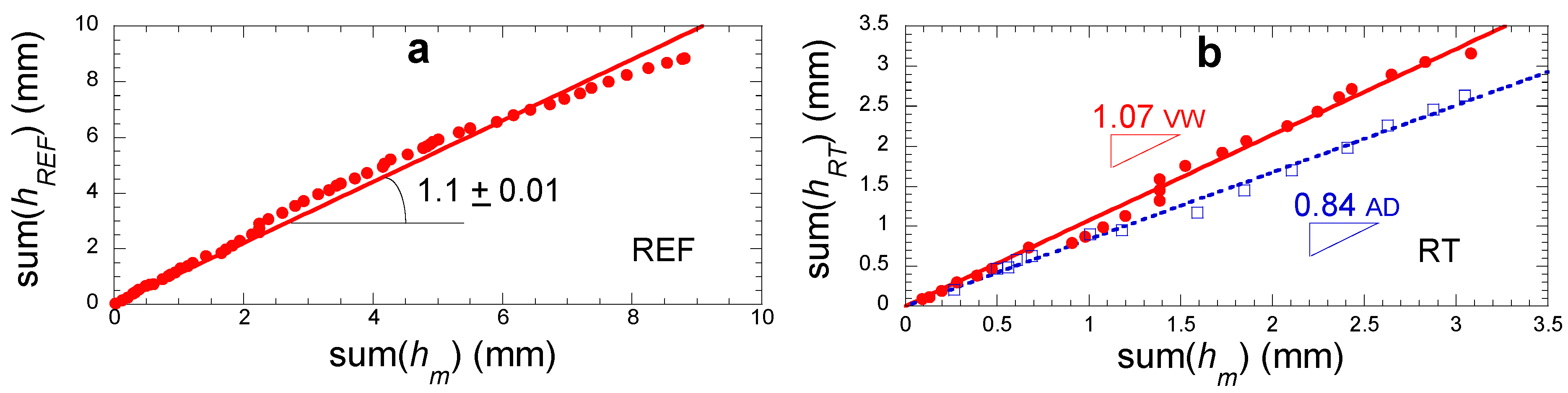
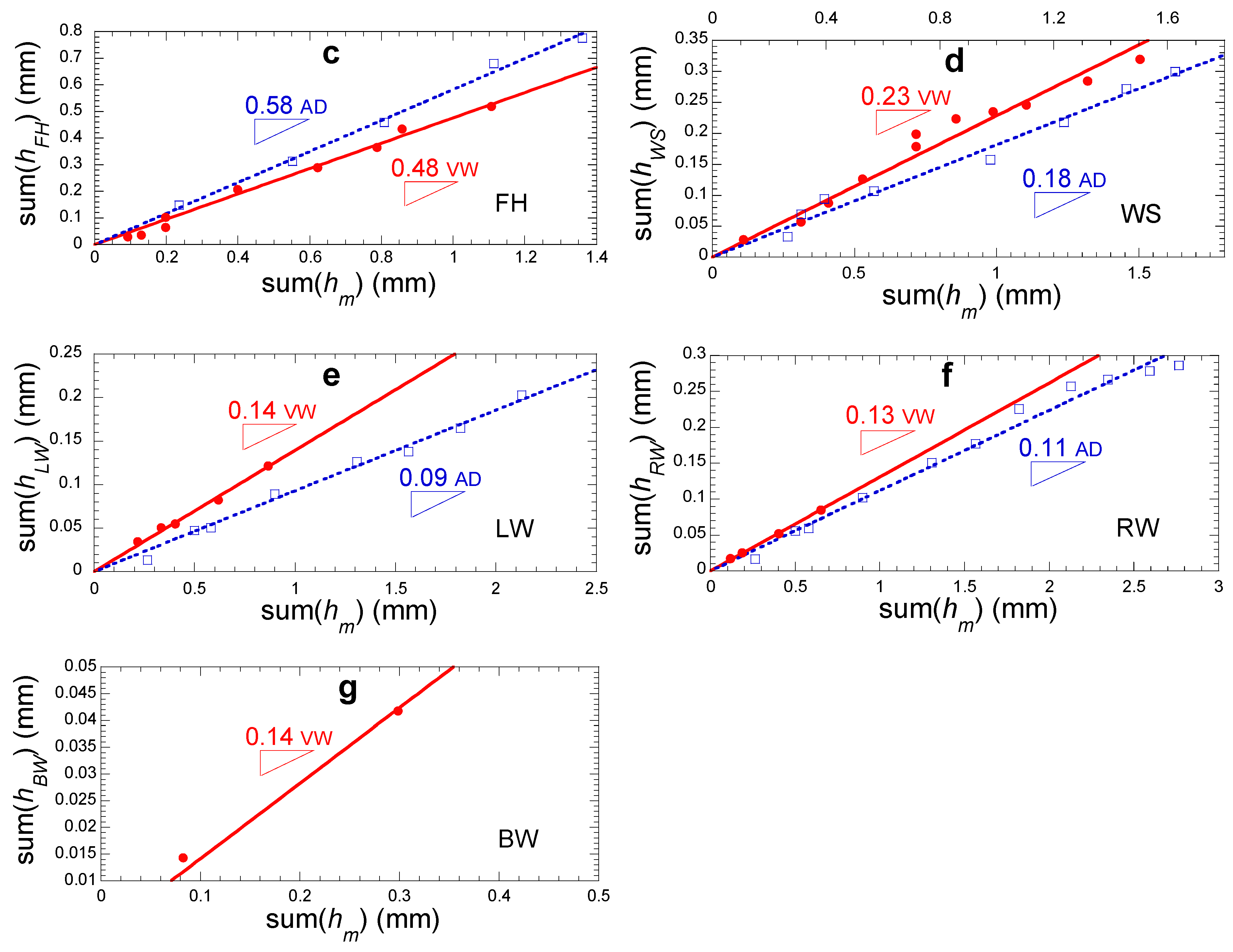
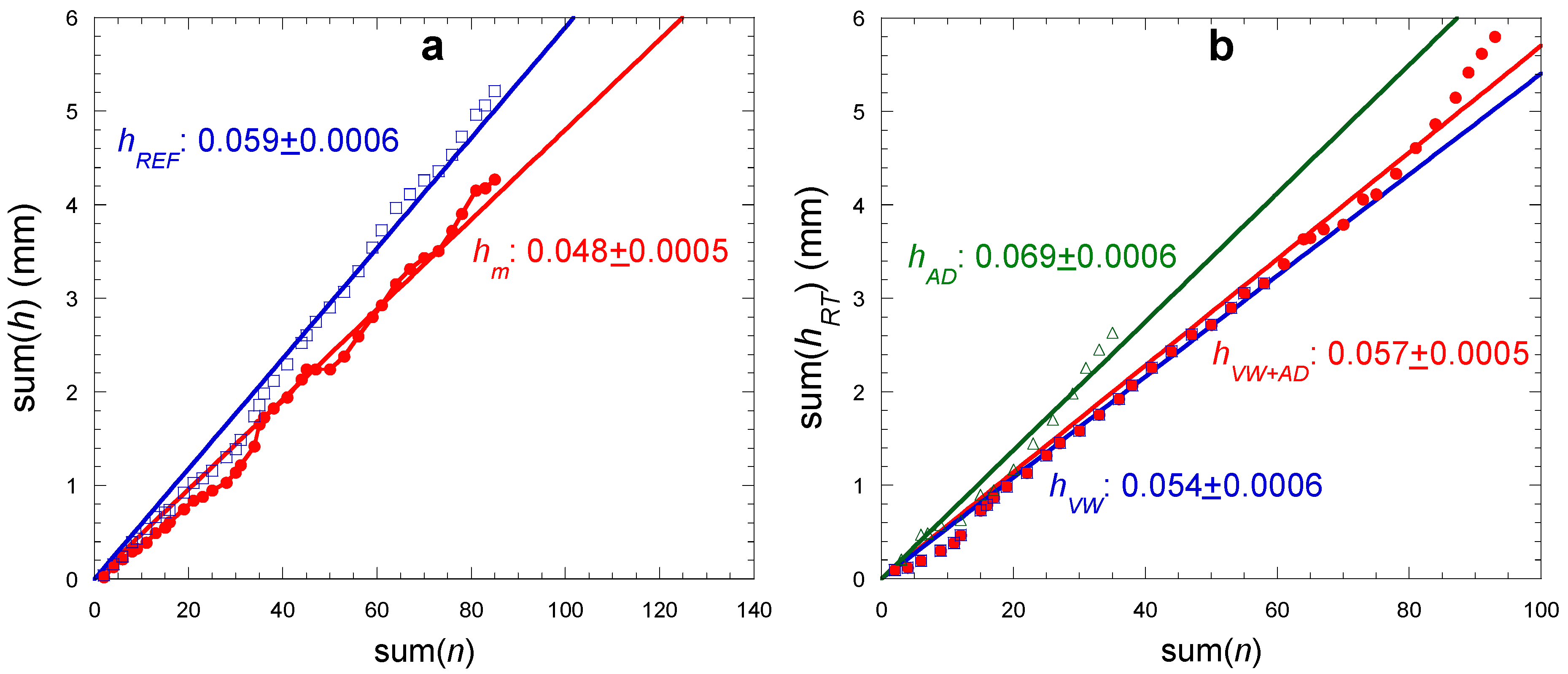
4.3. Dew Yield Estimation

4.3.1. Dew Yield from Surface Temperatures

The dew yield can be estimated from the condensing surface temperature T c and humid air dew point temperature T d (see, e.g., [6]). From Equation (28), one obtains, with Td in K:
h ˙ c = a ( φ ) ρ v γ T d ρ l ( T d T c )
The vapor density exhibits a relatively strong variation in the temperature range investigated (5–20 °C), and has to be expressed as a function of humid air dew point temperature and relative humidity through the equation of ideal gas. With rv = 462 J·kg−1·K−1 and p s ( T d ) = RH p s ( T a ) = p v ( T a ) , it becomes:
ρ v = p s ( T d ) 462 T d
In Figure 15 are shown the variations of the mean heat transfer coefficients with mean windspeed for the REF surface and the RT and FH surfaces of VW and AD cars. In this windspeed range (0–0.6 m·s−1), no clear variations were visible. These results were in agreement with the results of Section 4.2.2, where the effect of wind in a larger range (0–2.5) m·s−1 leads to only a weak increase of the heat transfer coefficient (Figure 9).
Figure 16a reports the variation of the temperature-dependent part h ˙ c T d / ρ v with respect to T d T c (Equation (38)). The expected proportionality is observed. The mean value of the reference surface as calculated from Equation (38) gives aREF = 2.2 ± 0.5 W·m−2·K−1. The calculated values of the other heat transfer coefficients aj with respect to surfaces tilt angle φ were reported for the three studied cars in Figure 16b. They were compared with the values calculated from the surface temperature measurements (Section 4.2.1 and Table 5) using the value aREF = 2.2 W·m−2·K−1. The shadow area in Figure 16b corresponds to the thermally isolated surfaces. The heat transfer coefficients outside this area slightly increased, as expected. This region was also the region where φ was larger, which confirms the observation in Section 4.2.1 of a constant heat transfer coefficient with respect to φ. The agreement between both sets of values was good for the same car and does not vary much between cars with a mean value of (2.75 ± 0.07) W·m−2·K−1 (VW), (3.15 ± 0.2) W·m−2·K−1 (AD) and 2.87 W·m−2·K−1 (DC). While VW and DC cars give nearly the same value, the AD car exhibits a larger value. All values were larger than the REF value (2.2 W·m−2·K−1) by 30–40% with a mean value of 2.92 W·m−2·K−1, in agreement with the calculations of Section 3.4 and Section 4.2.1. As in Section 3.4, one notes that the heat transfer coefficients of the AD car were systematically larger than the VW car, presumably because of enhanced air flows due to a different car geometry.

4.3.2. Dew Yield Estimation from Meteorological Data

The dew yield can be estimated from an energy balance model, which, thanks to the approximation TcTaTdTa in the expression of the heat losses with air, uses only a few classical meteorological data without adjustable parameters [8]: cloud cover N (oktas), windspeed at 10 m elevation (V, m·s−1), air temperature (Ta, °C), air relative humidity (RH, %) or dew point temperature (Td, °C). The results were concerned with dew yields h in mm per time ( Δ t ) 1 where Δ t corresponds to the time period in h. of the analyzed data. It was assumed that the substrate emissivity was unity (close to the emissivity ≈ 0.98 of a wet substrate, see [25]) and was thermally insulated from below. The formulation can be written as:
h m = ( Δ t 12 ) ( H L + R E )
The data for h < 0 corresponded to evaporation and were discarded. The quantity HL represents the convective heat losses between air and condenser assuming a heat transfer coefficient a = 3.5 W·m−2·K−1, corresponding to an ideal 1 m2 planar condenser, tilted 30° with horizontal, thermally isolated from below and with emissivity unity. There is a cut-off for windspeed V > V0 = 4.4 m·s−1 a value above which condensation vanishes:
h m = { ( Δ t 12 ) [ 0.06 ( T d T a ) + R E ]             if   V < V 0   0                                                                                                         if   V > V 0
The quantity RE is the available radiative energy, which depends on air–water content (measured by the dew point temperature Td, in °C), site elevation H (in km), and cloud cover N (in oktas):
R E = 0.37 × ( 1 + 0.204323 H 0.0238893 H 2 ( 18.0132 1.04963 H + 0.21891 H 2 ) × 10 3 T d ) ( T d + 273.15 285 ) 4 ( 1 N 8 )
The daily yields and their cumulated (sum) values were obtained after filtering the data from rain and fog events and integrating the time series on a daily time-step corresponding to h > 0. In Figure 17 are plotted the cumulated values sum(hj) of the measured dew yields hj on the reference and car rooftop surfaces, sum(hj), with respect to sum(hm). It shows that the calculated h m values slightly overestimate (10%) the measured values for the reference surface. This result is expected because the calculation corresponds to a 30° tilted plane where the dew yield was somewhat larger (~20%) than the horizontal surface yield [24]. The calculation underestimates (by 16%) the thermally isolated VW rooftop, due to an enhanced heat transfer coefficient with respect to a fully isolated surface. The calculation also underestimates the isolated AD rooftop and the other VW and AD surfaces due to the radiative cooling dependence with the tilt angle. The lower dew yields with the AD car, when compared to the VW car dew yields, can be attributed to the larger heat exchange coefficients, themselves the result of enhanced air flows due to a different car geometry (see Section 3.4 and Section 4.3.1, Table 5 and Figure 15 and Figure 16).

4.3.3. Comparison with the Visual Observation Scale

The visual observation scale summed on N events is defined by
sum ( n ) = p = 1 N n p
It is compared with the corresponding sum of dew yield as measured on a horizontal surface, where the dew yield is expected smaller by 20% from the same surface tilted at 30° [24],
sum ( h ) = p = 1 N h p
The comparison with visual observations following Equation (1) gives:
sum ( h ) = k sum ( n )
One expects the coefficient to be smaller than the coefficient K from Equation (1) because in Equation (45), the reference surface is horizontal. It thus becomes:
K = 1.2 k
Figure 18a reports the correlation between sum(n) and the sum(h) data as measured on the reference foil (sum(hREF)) or calculated from the meteo data (sum(hm)). Figure 18b compares the sum(n) data with the sum(hRT) measurements on VW and AD rooftops in Ajaccio. The value of the parameter k does not vary much around a mean value of k = 0.060, with the AD roof giving a value slightly larger (0.069). The previous study [15] reports a similar value k = 0.057 ± 0.03 for the comparison with rooftop measurements (see Table 6).
When compared with the hm calculated data in Ajaccio, which correspond to a plane tilted at 30° with horizontal, the value becomes smaller, K = 1.2 k = K = 0.048. The meteo data in Valparaiso for the night 28–29 April 2015 gave a calculated dew yield hm = 0.152 mm using [8] (Section 4.2.2). It corresponds to k = 0.042 or K = 0.051. Beysens et al. [15] found when using the calculated data hm a larger value K = 1.2 k = 0.067 (see Table 6). Data in Table 6 and Figure 19 show that the proportionality constant k can be taken as k ≈ 0.06 (horizontal planar surface) or equivalently K ≈ 1.2 k ≈ 0.07. The uncertainty was less than 20%.

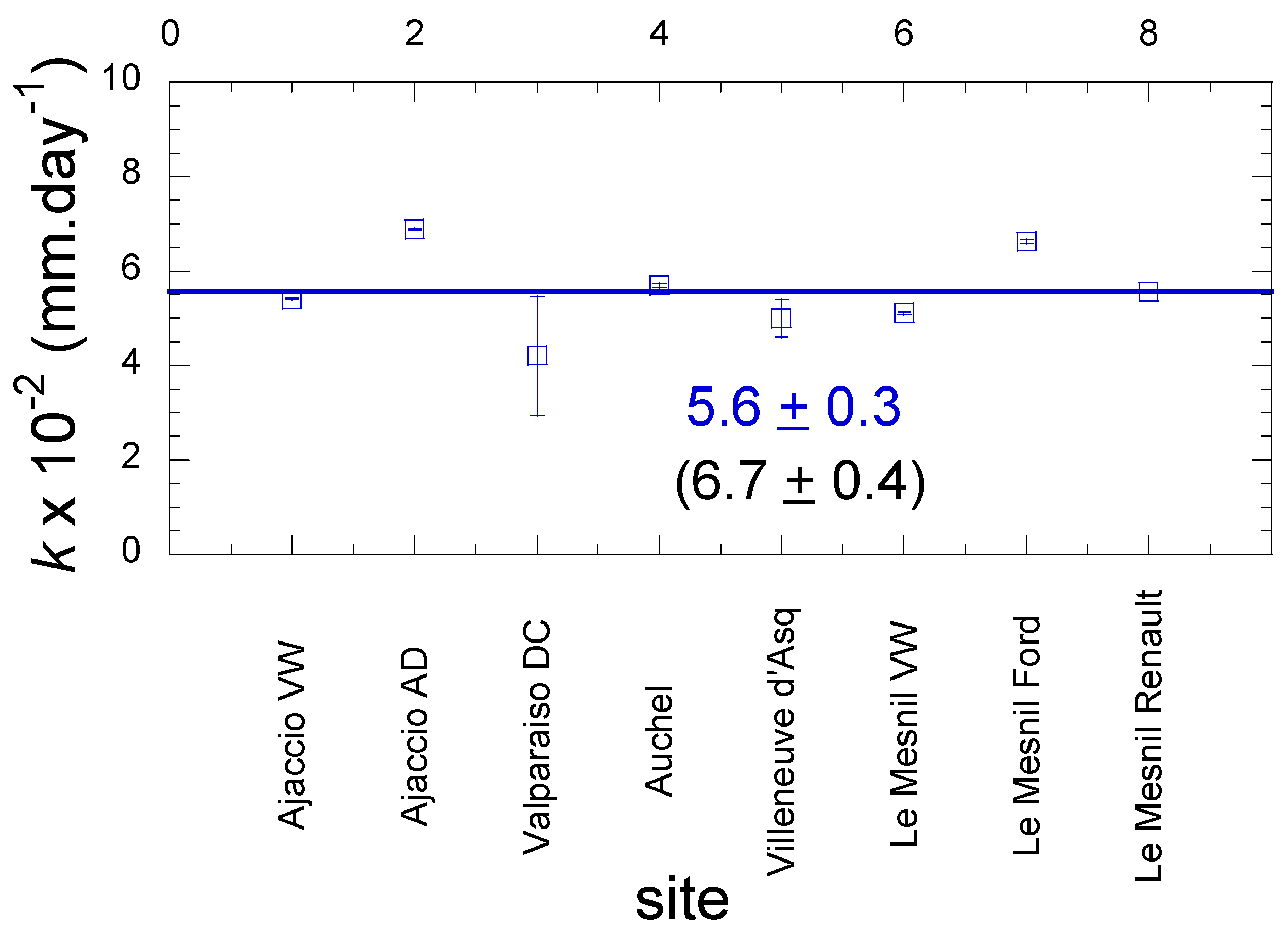
4.3.4. Variability Climate—Car Trade Mark

Table 7 summarizes the different studies made with six different cars in five different locations corresponding to three different climates, with the determined values of proportionality factor k for an isolated horizontal surface. These values are reported in Figure 19. They are randomly scattered around the mean value k = (0.056 ± 0.3) mm·day−1 (uncertainty: one standard deviation), a value corresponding to the factor K = 1.2 k = (0.067 ± 0.36) mm·day−1 for a 30° tilted, thermally isolated, planar condenser.

5. Conclusions

From this study, one concludes that cars can be used as standard condensers for estimating the dew yield. Car surfaces indeed permit detailed studies of radiative cooling and dew formation on planar and tilted surfaces, thermally and not thermally isolated, in the presence of obstacles and wind. Cars indeed exhibit horizontal or near horizontal surfaces (rooftop, front hood, back trunk) and inclined surfaces (windshield, lateral windows, back window) surfaces with thermally isolated (rooftop, front hood) or not thermally isolated surfaces (windshield, lateral windows, back window). In addition, the infra-red emissivities of all surfaces are nearly the same and close to water’s once wet, that is, near unity (0.98 in the atmospheric window).
Cooling and dew condensation on car surfaces are seen to depend on surface thermal isolation, tilt angle-dependent radiation deficit, and heat and mass transfer coefficients, which are seen as being proportional to each other. Temperature and dew yield measurements give heat transfer coefficient nearly independent of windspeed and tilt angle (reference plane mean value: 2.2 W·m−2·K−1; car mean value: 2.9 W·m−2·K−1).
A visual observation scale n = 0, 1 2, 3, depending on whether dew form or not on rooftop, windshield and lateral windows, is used as a proxy for nightly dew yield evaluation. The relation h (mm/day) = Kn is validated with K = (0.067 ± 0.0036) mm·day−1. The results are robust, supported by the study of eight different cars in five different sites with three different climates.

Author Contributions

Conceptualization, M.M. and D.A.B.; Data curation, M.M. and D.A.B.; Formal analysis, M.M. and D.A.B.; Funding acquisition, D.A.B.; Investigation, M.M. and D.C.; Methodology, M.M., D.C. and D.A.B.; Supervision, D.A.B.; Writing—original draft, M.M. and D.A.B.; Writing—review & editing, M.M., D.C. and D.A.B. All authors have read and agreed to the published version of the manuscript.

Funding

This research received no external funding.

Institutional Review Board Statement

Not applicable.

Informed Consent Statement

Not applicable.

Data Availability Statement

Not applicable.

Acknowledgments

OPUR (www.opur.fr, accessed on 1 December 2021) is gratefully acknowledged for D.A.B and M.M. financial support.

Conflicts of Interest

The authors declare no conflict of interest.

References

  1. Monteith, J.L. Dew. Q. J. Royal. Meteorol. 1957, 83, 322–341. [Google Scholar] [CrossRef]
  2. Tomaszkiewicz, M.; Abou Najm, M.; Zurayk, R.; El-Fadel, M. Dew as an Adaptation Measure to Meet Water Demand in Agriculture and Reforestation. Agric. For. Meteorol. 2017, 232, 411–421. [Google Scholar] [CrossRef]
  3. Fang, J. A review on eco-hydrological effects of condensation water. Sci. Cold Arid Reg. 2013, 5, 275–281. [Google Scholar]
  4. Tomaszkiewicz, M.; Abou Najm, M.; Beysens, D.; Alameddine, I.; El-Fadel, M. Dew as a sustainable non-conventional water resource: A critical review. Environ. Rev. 2015, 23, 425–442. [Google Scholar] [CrossRef]
  5. Kaseke, K.F.; Wang, L. Fog and dew as potable water resources: Maximizing harvesting potential and water quality concerns. GeoHealth 2018, 2, 327–332. [Google Scholar] [CrossRef]
  6. Beysens, D. Dew Water; Rivers Publisher: Gistrup, Denmark, 2018. [Google Scholar]
  7. Vuollekoski, H.; Vogt, M.; Sinclair, V.A.; Duplissy, J.; Järvinen, H.; Kyrö, E.M.; Makkonen, R.; Petäjä, T.; Prisle, N.L.; Räisänen, P.; et al. Estimates of global dew collection potential on artificial surfaces. Hydrol. Earth. Syst. Sci. 2015, 19, 601–613. [Google Scholar] [CrossRef] [Green Version]
  8. Beysens, D. Estimating dew yield worldwide from a few meteo data. Atmos. Res. 2016, 167, 146–155. [Google Scholar] [CrossRef]
  9. Recent Observed Changes in Extreme High-Temperature Events and Associated Meteorological Conditions over Africa. Int. J. Climatol. Available online: https://doi.org/10.1002/joc.7485 (accessed on 1 December 2021).
  10. Iyakaremye, V.; Zeng, G.; Yang, X.; Zhang, G.; Ullah, I.; Gahigi, A.; Vuguziga, F.; Gebremariam Asfaw, T.; Ayugi, B. Increased high-temperature extremes and associated population exposure in Africa by the mid-21st century. Sci. Total Environ. 2021, 790, 148162. [Google Scholar] [CrossRef] [PubMed]
  11. Tomaszkiewicz, M.; Abou Najma, M.; Beysens, D.; Alameddine, I.; Bou Zeid, E.; El-Fadel, M. Projected climate change impacts upon dew yield in the Mediterranean basin. Sci. Total Environ. 2016, 566–567, 1339–1348. [Google Scholar] [CrossRef]
  12. Agam, N.; Berliner, P. Dew formation and water vapor adsorption in semi-arid environments—A review. J. Arid Environ. 2006, 65, 572–590. [Google Scholar] [CrossRef]
  13. Lekouch, I.; Lekouch, K.; Muselli, M.; Mongruel, A.; Kabbachi, B.; Beysens, D. Rooftop dew, fog and rain collection in southwest Morocco and predictive dew modeling using neural networks. J. Hydrol. 2012, 448, 60–72. [Google Scholar] [CrossRef]
  14. Valjarević, A.; Filipović, D.; Valjarević, D.; Milanović, M.; Milošević, S.; Živić, N.; Lukić, T. GIS and remote sensing techniques for the estimation of dew volume in the Republic of Serbia. Meteorol. Appl. 2020, 27, e1930. [Google Scholar] [CrossRef]
  15. Beysens, D.; Pruvost, V.; Pruvost, B. Dew observed on cars as a proxy for quantitative measurements. J. Arid Environ. 2016, 135, 90–95. [Google Scholar] [CrossRef] [Green Version]
  16. Muselli, M.; Beysens, D.; Marcillat, J.; Milimouk, I.; Nilsson, T.; Louche, A. Dew water collector for potable water in Ajaccio (Corsica Island, France). Atmos. Res. 2002, 64, 297–312. [Google Scholar] [CrossRef]
  17. OPUR. 2021. Available online: www.opur.fr (accessed on 1 December 2021).
  18. Nilsson, T.M.J.; Vargas, W.E.; Niklasson, G.A.; Granqvist, C.G. Condensation of water by radiative cooling. Renew. Energy 1994, 5, 310–317. [Google Scholar] [CrossRef]
  19. Hall, J.N.; Fekete, J.R. Steels for auto bodies. In Automotive Steels; Woodhead Publishing: Cambridge, UK, 2017. [Google Scholar]
  20. The Engineering Toolbox. 2021. Available online: https://www.engineeringtoolbox.com (accessed on 1 December 2021).
  21. Raghu, O.; Philip, J. Thermal properties of paint coatings on different backings using a scanning photo acoustic technique. Meas. Sci. Technol. 2006, 17, 2945–2949. [Google Scholar] [CrossRef]
  22. Downing, H.; Williams, D. Optical constant of water in the infrared. J. Geophys. Res. 1975, 80, 1656–1661. [Google Scholar] [CrossRef]
  23. Pal Arya, S. Introduction to Micrometeorology; Academic Press: San Diego, CA, USA, 1988. [Google Scholar]
  24. Beysens, D.; Milimouk, I.; Nikolayev, V.; Muselli, M.; Marcillat, J. Using radiative cooling to condense atmospheric vapor: A study to improve water yield. J. Hydrol. 2003, 276, 1–11. [Google Scholar] [CrossRef]
  25. Trosseille, J.; Mongruel, A.; Royon, L.; Beysens, D. Effective surface emissivity during dew water condensation. Int. J. Heat Mass Transf. 2022, 183, 122078. [Google Scholar] [CrossRef]
  26. Bliss, R.A. Atmospheric radiation near the surface of the ground. Sol. Energy 1961, 5, 103–120. [Google Scholar] [CrossRef]
  27. Berger, X.; Bathiebo, J. Clear sky radiation as a function of altitude. Int. J. Renew. Energy 1992, 2, 139–157. [Google Scholar] [CrossRef]
  28. Awanou, C.N. Clear sky emissivity as a function of the zenith direction. Renew. Energy 1998, 13, 227–248. [Google Scholar] [CrossRef]
  29. Berger, X.; Bathiebo, J. Directional spectral emissivities of clear skies. Renew. Energy 2003, 28, 1925–1933. [Google Scholar] [CrossRef]
  30. Howell, J.C.; Yizhaq, T.; Drechsler, N.R.; Zamir, Y.; Beysens, D.; Shaw, J.A. Radiative, Power-Enhanced Dew Collection. J. Hydrol. 2021, 603, 126971. [Google Scholar] [CrossRef]
  31. Clus, O.; Ortega, P.; Muselli, M.; Milimouk, I.; Beysens, D. Study of dew water collection in humid tropical islands. J. Hydrol. 2008, 361, 159–171. [Google Scholar] [CrossRef]
  32. Sokuler, M.; Auernhammer, G.K.; Liu, C.J.; Bonaccurso, E.; Butt, H.-J. Dynamics of condensation and evaporation: Effect of inter-drop spacing. Europhys. Lett. 2010, 89, 36004. [Google Scholar] [CrossRef]
  33. Beysens, D.; Muselli, M.; Nikolayev, V.; Narhe, R.; Milimouk, I. Measurement and modelling of dew in island, coastal and alpine areas. Atmos. Res. 2005, 73, 1–22. [Google Scholar] [CrossRef] [Green Version]
  34. Clus, O.; Ouazzani, J.; Muselli, M.; Nikolayev, V.S.; Sharan, G.; Beysens, D. Comparison of Various Radiation-cooled Dew Condensers Using Computational Fluid Dynamics. Desalination 2009, 249, 707–712. [Google Scholar] [CrossRef]
  35. Sharan, G.; Roy, A.K.; Royon, L.; Mongruel, A.; Beysens, D. Dew plant for bottling water. J. Clean. Prod. 2017, 155, 83–92. [Google Scholar] [CrossRef]
  36. Beysens, D.; Cooke, R.; Crobu, E.; Royon, L. Computational Fluid Dynamics study of a corrugated hollow cone for enhanced dew yield. J. Hydrol. 2021, 592, 125788. [Google Scholar] [CrossRef]
  37. Lienhard, J.H., IV; Lienhard, J.H., V. A Heat Transfer Textbook, 5th ed.; Dover Publications Inc.: Mineola, NY, USA, 2019. [Google Scholar]
  38. Guyon, E.; Hulin, J.-P.; Petit, L. Hydrodynamique Physique, 3rd ed.; EDP Sciences: Paris, France, 2012. (In French) [Google Scholar]
  39. Schlichting, H. Boundary Layer Theory, 9th ed.; Springer: Berlin/Heidelberg, Germany, 2017. [Google Scholar]
  40. Rohsenow, W.M.; Hartnett, J.R.; Cho, Y.I. Handbook of Heat Transfer, 3rd ed.; Mc Graw-Hill: New York, NY, USA, 1998. [Google Scholar]
  41. MIT. 2016. Available online: http://web.mit.edu/16.unified/www/FALL/thermodynamics/notes/node64.html (accessed on 1 December 2021).
  42. Nikolayev, V.; Beysens, D.; Gioda, A.; Milimouk, I.; Katiushin, E.; Morel, J. Water recovery from dew. J. Hydrol. 1996, 182, 19–35. [Google Scholar] [CrossRef] [Green Version]
  43. Sharan, G.; Clus, O.; Singh, S.; Muselli, M.; Beysens, D. A very large dew and rain ridge collector in the Kutch area (Gujarat, India). J. Hydrol. 2011, 405, 171–181. [Google Scholar] [CrossRef]
Figure 1. (a) Definition of the apparent angle above horizontal α of nearby obstacles, angle φ of the condensing surface S with horizontal, skyview angle SV, and sky radiation angle θ with vertical. (bd) Effect of obstacle radiations from ground and obstacles (angle α + φ) and skyview limitation (angle 180° − αφ). Other notations: see text.
Atmosphere 13 00065 g001
Figure 2. Experimental sites. (a) Ajaccio site. 1: VW and AD cars, oriented SSE; 2: nearby parked car; 3: planar condenser used as a reference; 4: meteorological station. The North direction is indicated by the black arrow. (From Google Earth, 1 October 2020). (b) Valparaiso. The arrow indicates the DC car location and the cross the meteo station. (From Google Earth, 1 August 2019).
Atmosphere 13 00065 g002
Figure 3. (a). Mean number of events with respect to the wind direction at night (21 h−7 h) between 15 July and 30 November 2020. Orange lines: all nights; blue line: only nights with dew events. (b) The corresponding distribution of windspeed at 10 m.
Atmosphere 13 00065 g003
Figure 4. Characteristics of (a) windshield, (b) other windows (c) roof top, and (d) reference condenser. Thicknesses are denoted by e, thermal conductivity by λ, heat transfer coefficients by a, temperatures by T. Subscripts correspond to: a—air, g—glass, s—sandwich film, p, rooftop metal, i, thermal isolation, b—ground basis. Superscripts ‘ and ‘’ correspond to different values. Ri is the radiative deficit flux.
Atmosphere 13 00065 g004
Figure 5. Cars under study with the position of the K-thermocouple sensors. (a,b): VW and AD cars (Ajaccio, France); (c): DC car (Valparaiso, Chile). (Scale and actual angles are not respected on pictures).
Atmosphere 13 00065 g005
Figure 6. (a) Directional emissivity ε θ with respect to angle θ with vertical for different total emissivities ε s (Equation (11) with b = 1.8). The interrupted vertical lines (A) corresponds to the influence of the nearby vehicle in the NNE direction, with emissivity near unity. The double interrupted vertical line (B) corresponds to the influence of the nearby buildings in nearly all directions, with emissivity near unity. The continuous vertical lines (C) corresponds to the limiting sky views related to the windows tilt angles φ. (b) Variation with tilt angle φ of radiation deficit in Ajaccio at T = 15 °C with no obstacles, corresponding to the precipitable water vapor PWV = 0.78 cm (data interpolated from [31]). The vertical lines correspond to the window’s tilt angles. (c) Variation with respect to the tilt angle of the relative radiative deficit R i ( α ,   φ ) / R i ( 0 , 0 ) at various obstacle view angles α (data interpolated from [30]).
Atmosphere 13 00065 g006
Figure 7. Night temperature evolution of outside air temperature, Ta, temperature inside the car Ta, dew point temperature Td, rooftop temperature, TRT, windshield temperature, TWS, and difference TRTTa. (a) VW car in Ajaccio (23–24 April 2021, time UT + 2). (b) DC car in Valparaiso (28–29 April 2015, time UT − 3).
Atmosphere 13 00065 g007
Figure 8. Recorded data for the reference condenser (T0) and left and right windows on the AD car for the night 6–7 November 2020 (hh:mm:ss, UT + 1) in Ajaccio. (a) Differences with air temperature Ta of the temperatures of reference (T0), left (TLW), and right (TRW) windows. (b) Corresponding windspeed V and wind direction Dir V. (c) Cooling efficiency ratio Δ T L W * and Δ T R W * (left and right windows, respectively). (d): Left and right window cooling with respect to air temperature (TLW,RWTa) as a function of windspeed V10 extrapolated at 10 m from the ground. Curves are smoothing functions. During this night, dew yields were (REF) hREF = 0.265 mm·day−1, (LW) hLW = 0.039 mm·day−1 and (RW) hRW = 0.043 mm·day−1, corresponding in the visual scale to n = 3 (≈ 0.17 mm·day−1 using the factor 0.056 mm·day−1 from Section 4.3.4).
Atmosphere 13 00065 g008aAtmosphere 13 00065 g008b
Figure 9. Recorded data for the reference condenser (T0) and rooftop and front hood on the AD car for the night 13–14 November 2020 (hh:mm:ss, UT + 1) in Ajaccio. (a) Differences with air temperature Ta of the temperatures of reference (T0), rooftop (TRT), and front hood (TFH). (b) Corresponding windspeed V and wind direction Dir V. (c) Cooling efficiency ratio Δ T R T * and Δ T F H * (roof top and front hood, respectively). (d): Roof top and front hood cooling (TRT,FHTa) with respect to air temperature Ta as a function of windspeed V10 extrapolated at 10 m from the ground. Curves are smoothing functions. During this night, dew yields were (REF) hREF = 0.197 mm, (RT) hRT = 0.148 mm and (FH) hFH = 0.043 mm, with n = 2 (≈0.11 mm·day−1 using the factor 0.056 mm·day−1 from Section 4.3.4).
Atmosphere 13 00065 g009
Figure 10. Recorded data from rooftop RT, back trunk BT, windshield WS, back window BW of the DC car in Valparaiso during the night 28–29 April 2015 (hh:mm:ss, UT-3). (a) Differences with air temperature Ta of the temperatures of rooftop (TRT), back trunk (TBT), windshield (TWS), and back window (TBW). (b) Corresponding windspeed V and wind direction Dir V. (c) Cooling efficiency ratio Δ T R T * , Δ T B T * , Δ T W S * and Δ T B W * . Roof top value is, by definition, constant and equal to 0.8 (Equation (3)). (d): Roof top, back trunk, windshield, back window cooling (TTa) as a function of windspeed V10 extrapolated at 10 m from the ground. Curves are smoothing functions. During this night, n = 3 (≈0.17 mm·day−1 using the factor 0.056 mm·day−1 from Section 4.3.4). The calculated dew yield using [8] of Section 4.2.2 gives (REF) hREF = 0.15 mm.
Atmosphere 13 00065 g010
Figure 11. Daily mean relative cooling efficiencies Δ T * and daily dew yield hc (mm·day−1) for the different car surfaces during condensation (TjTd) < 0 in Ajaccio. Error bars correspond to one SD. (a) rooftop RT; (b) front hood FH; (c) windshield WS; (d) left window LW; (e) right window RW; (f) back window BW; Δ T *   data: Full squares (VW) and open squares (AD). Dew yield data: Dark bars (VW) and light bars (AD). The value for Valparaiso is indicated for comparison by a red circle (BT is compared with FH).
Atmosphere 13 00065 g011
Figure 12. Variation with tilt angle φ of the temperature efficiency Δ T * for the VW, AD, and DC cars, fitted to Equation (30) by using the polynomial functions Equations (32) and (33) with a j / a 0 as adjustable parameters (curves). The isolated surfaces (RT, FH) are fitted separately from the non-isolated surfaces (WS, BW, LW). (a) Mean values for the VW car in Ajaccio. (b) Mean values for the AD car in Ajaccio. (c) DC car in Valparaiso. Red full circle and continuous curve: RT thermally isolated surface and obstacle view angle α 0 ° . Blue open triangle and dotted curve: Non-isolated BW surface and α 0 ° . Brown inverted triangle and double-interrupted curve: Non-isolated WS surfaces and α 30 ° . Green open square and interrupted curve: Non-isolated BT surface and α 30 ° .
Atmosphere 13 00065 g012aAtmosphere 13 00065 g012b
Figure 13. Instantaneous values of j-inverse surface temperature difference with air, ( T a T j ) 1 a j , the j-heat transfer coefficient, with respect to mean windspeed value V10 at 10 m off the ground. Data are taken during condensation (Tj < Td). (a) Reference foil, (b) rooftop, (c) front hood, (d) windshield, (e) back window, (f) left window, (g) right window. VW (red dots and continuous curves) and AD (blue dots and interrupted curves) cars are considered separately. The curves are smoothing functions.
Atmosphere 13 00065 g013
Figure 14. (a) Windspeed versus wind direction during dew formation (Tj < Td). (bh) Instantaneous values of j- inverse surface temperature difference with air ( T a T j ) 1 ~   a j , the j-heat transfer coefficient, with respect to wind direction Dir(V) during condensation (Tj < Td). (b) Reference foil, (c) rooftop, (d) front hood, (e) windshield, (f) back window, (g) left window, (h) right window. VW and AD cars are both considered.
Atmosphere 13 00065 g014
Figure 15. Variation of the heat transfer coefficients with windspeed. (a) REF surface. (b) VW and AD rooftop and front hood surfaces. VW car: Red circles (RT) and brown triangles (FH). AD car: Blue square (RT) and light blue diamond (FH).
Atmosphere 13 00065 g015
Figure 16. (a) Variation of h ˙ c T d / ρ v with respect to T d T c for the Ajaccio reference surface. The proportionality factor is (3.14 ± 0.09) × 10−5 m4·K.s−1·Kg−1 (uncertainty: one standard deviation) corresponding to the value aREF = 2.2 W·m−2·K−1. (b) Calculated heat transfer coefficient at different angles as calculated from (full symbols) the aj/aREF values from temperature measurements (Section 4.2.1, Table 5) with aREF = 2.2 W·m−2·K−1, and the means of h ˙ c / ( T d T c ) data from Equation (38) (values from Table 6, open symbols). VW car: red circles, full and dotted lines. AD car: squares, interrupted, and double interrupted lines. DC car: Green triangles and large interrupted line. REF: Black diamond. The shadow area corresponds to thermally isolated surfaces.
Atmosphere 13 00065 g016
Figure 17. Comparison between the calculated sum of dew yields from meteo data (sum(hm)) and experimental values (a) from the reference surface (sum(hREF)) and the VW and AD car surfaces: (b) RT, (c) FH, (d) WS, (e) LW, (f) RW, and (g) BW. The data are fitted to sum(hj) = λj sum(hm). The λj values are noted in the figures. Standard deviations are ≈ 0.01. Red dots: VW car; blue open squares: AD car.
Atmosphere 13 00065 g017aAtmosphere 13 00065 g017b
Figure 18. (a) Variation of sum(hm) (red dots) and sum(hREF) (blue open squares) as a function of the visual scale sum(n). The values correspond to the result of linear fits (straight lines, uncertainties: One SD). (b) Variation of sum(hRT) for VW rooftop (blue open squares), AD rooftop (green open triangles) and VW + AD rooftops (red dots). The values correspond to the result of linear fits (straight lines, uncertainties: One SD).
Atmosphere 13 00065 g018
Figure 19. Values of factor k between dew yield on a thermally isolated horizontal plane and from the observation scale (Equations (1) and (43)–(45)) as a function of measurement site and type of car. The mean value k = 0.056 ± 0.003 mm·day−1 is indicated with one standard deviation uncertainty. The value under the bracket is for comparison with a thermally isolated 30° inclined plane and corresponds to K = 1.2 k = 0.067 ± 0.0036 mm·day−1.
Atmosphere 13 00065 g019
Table 1. Meteorological specific information for both test locations. (§): The wind speed is higher than measured at the measurement site because the meteo station is located at the top of a hill (Aeródromo Rodelillo, Viña del Mar).
AjaccioValparaίso
Latitude41°57′57″ N33°18′00″ S
Longitude8°48′43″ E71°31′48″ W
Altitude (m asl)53340
Average high temperature (°C)20.518.7
Average low temperature (°C)10.59.1
Mean temperature (°C)15.413.9
Average relative humidity (%)6976
Average wind velocity (m·s−1)3.55.9 §
Average rainfall (mm·year−1)723365
Table 2. View angle of obstacles seen from the right, left, back, front of the vehicle (αi) and parked along the vehicle (αi) (see Figure 2a).
Obstacle
Angle
α1 (°)
Right
α2 (°)
Left
α3 (°)
Back
α4 (°)
Front
α5 (°)
Front Hood
α6 (°)
Back Trunk
α′2 (°)
Left
Car
VW1.24.4232.320-8
AUDI
DC2.41.88.240-337.5
REF.north:
17.7
east:
11.3
south:
11.3
west:
≈0
---
Table 4. Summary of studied car surfaces properties: Tilt angle, presence of thermal isolation, approximations used for the view angles of obstacles seen from the different car surfaces (from Table 2). Angles are counted in the trigonometric order. RT: rooftop; FH: front hood; BT: back trunk; WS: windshield; LW: left window; RW: right window; BW: back window.
CarsVWADDC
Car PartRTFHWSLWRWBWRTFHWSLWRWBWRTBTWSBW
Approx. view angle α (°)000000000000030300
Surface tilt φ (°)−1143068−68−440112961−61−350−330−47
Thermal isolationYYNNNNYYNNNNYNNN
Table 5. Tilt angles φ , sky view SV and cooling efficiencies Δ T * ¯ according to the different condensing surfaces for three different vehicles. SD: standard deviation. (§): virtual reference computed in Section 2.1.2.
Surface
Model
RTFHBTWSLWRWBW
VW φ (°)−1−14 −3068−6844
Event nb.1310 15121011
S V (°)180164 148104111113
Δ T * ¯ 0.860.81 0.630.380.410.64
SD0.030.03 0.030.020.030.01
aNI/a0 1.39 ± 0.031.40 ± 0.041.30 ± 0.041.19 ± 0.02
1.29 ± 0.03
aI(0)/a01.18 ± 0.02-
h ¯ 0.1320.058 0.0290.0240.0210.021
SD0.0530.031 0.0530.0310.0530.031
AD φ (°)0−11 −2961−6135
Event nb.1112 13997
S V (°)180167 149111118125
Δ T * ¯ 0.730.69 0.570.370.380.50
SD0.040.03 0.040.040.040.05
aNI/a0 1.55 ± 0.061.62 ± 0.11.58 ± 0.11.68 ± 0.08
1.61 ± 0.06
aI(0)/a01.40 ± 0.02-
h ¯ 0.1880.155 0.0470.040.060.04
SD0.0580.04 0.0370.0180.0260.019
DC φ (°)0-3−30--47
Event nb.1 11--1
S V (°)132 139110--130
Δ T * ¯ 0.80 §0.370.620.50--0.53
SD00.060.080.07--0.06
aNI/a0 1.34 ± 0.11.31 ± 0.25--1.33 ± 0.05
1.33 ± 0.05
aI(0)/a01.24 ± 0.05-
ReferenceTypeAjaccioValparaiso—Virtual
φ (°)00
S V (°)180180
h ¯ 0.170.13 §
SD0.060.03
Table 6. Mean values of heat transfer coefficients from surface temperature using the value aREF (bold) = 2.2 W·m−2·K−1 in Table 5, and from condensation rates using Equation (38). The mean values are highlighted in bold.
CarHeat Transfer Coefficients
From Surface TemperaturesFrom Conden-
Sation Rates
ValueSDValueSD
REF--2.20.5
VW2.80.12.70.3
AD3.30.13.00.4
DC2.870.05--
Mean car2.920.04
Table 7. Summary of studies made with cars indicating sites with Köppen-Geiger climate classification, time of the study, reference surface, car type and color, car surface tilt angles (absolute values), and proportionality constant k between dew yield and observation scale (Equations (1) and (43)–(45)). a This study. b Data from [15]. c Uncertainty estimated to 30%.
Site Coordinates
Köppen-Geiger Climate
Measur.Time
(mm/dd/yy)
Reference Surface, Tilt from HorizontalCar type and ColorRT Angle
(°)
WS Angle
(°)
LW Angle
(°)
RW Angle
(°)
BW Angle
(°)
FH Angle
(°)
BT Angle
(°)
k
(× 10 −2 mm)
Ajaccio (France)
8°48′43″ E, 41°57′57″ N
Am
07/15/20–10/25/200.5 m², 0°a Volkswagen Polo, 2016, white−1−3068−6844−14-5.41± 0.015.70 ± 0.05
10/29/20–11/30/200.5 m², 0°a Audi A3, 2020, gray0−2961−6135−11-6.89 ± 0.02
Valparaiso
(Chile)
71°34′46″ W, 33°7′9″ S
Csb
04/28-29/15 (one night)virtuala Daihatsu Charade, 1991, white0−30--47-3c 4.2 ± 1.3
Auchel (France)
2°27′9″ E,
50°30′59″ N
Cfb
2/15/2015–5/13/2015-b Peugeot 206 hdi, 2006, red-−2169−69---5.70 ± 0.045.66 ± 0.03
Villeneuve d’Asq (France)
3°8′3″ E, 50°37′43″ N
Cfb
3/18/15–3/27/15-b Opel Corsa C, 2006, dark blue-−2868−68---5.0 ± 0.4
Le Mesnil-en-Thelle
2°17′10″ E, 49°10′41″ N
Cfb
1/1/11–12/31/13-b Volkswagen Golf GTI, 1991, white-−3470−70---5.11 ± 0.035.553 ± 0.003
1/1/14–9/30/14-b Opel Corsa C, 2006, dark blue-−3068−68---6.63 ± 0.05
1/1/2011–9/30/2014-b Renault
Scenic 2009,
black
-−2870−70
Publisher’s Note: MDPI stays neutral with regard to jurisdictional claims in published maps and institutional affiliations.

