Article

Santa Ana Winds: Fractal-Based Analysis in a Semi-Arid Zone of Northern Mexico

by
Yeraldin Serpa-Usta
1,
Alvaro Alberto López-Lambraño
1,2,3,*,
Dora-Luz Flores
1,
Ena Gámez-Balmaceda
2,3,
Luisa Martínez-Acosta
4,
Juan Pablo Medrano-Barboza
4,
John Freddy Remolina López
5,
Alvaro López-Ramos
4 and
Mariangela López-Lambraño
6
1
Faculty of Engineering, Architecture and Design, Universidad Autónoma de Baja California, Ensenada 22860, Mexico
2
Hidrus S.A. de C.V., Ensenada 22760, Mexico
3
Grupo Hidrus S.A.S., Monteria 230002, Cordoba, Colombia
4
GICA Group, Faculty of Civil Engineering, Universidad Pontificia Bolivariana Campus Monteria, Monteria 230002, Cordoba, Colombia
5
ITEM Group, Faculty of Electronic Engineering, Universidad Pontificia Bolivariana Campus Monteria, Monteria 230002, Cordoba, Colombia
6
Business School, Universidad del Norte, Barranquilla 081007, Atlantico, Colombia
*
Author to whom correspondence should be addressed.
Atmosphere 2022, 13(1), 48; https://doi.org/10.3390/atmos13010048
Submission received: 29 October 2021 / Revised: 21 December 2021 / Accepted: 24 December 2021 / Published: 28 December 2021
(This article belongs to the Special Issue Feature Papers in Atmosphere Science)

Abstract

:
A fractal analysis based on the time series of precipitation, temperature, pressure, relative humidity, and wind speed was performed for 16 weather stations located in the hydrographic basin of the Guadalupe River in Baja California, Mexico. Days on which the phenomenon known as Santa Ana winds occurs were identified based on the corresponding criteria of wind speed (≥4.5 m/s) and wind direction (between 0° and 90°). Subsequently, the time series was formed with data representing the days on which this phenomenon occurs in each of the analyzed weather stations. A time series was additionally formed from the days in which the Santa Ana winds condition does not occur. Hurst exponents and fractal dimension were estimated applying the rescaled range method to characterize the established time series in terms of characteristics of persistence, anti-persistence, or randomness along with the calculation of the climate predictability Index. This enabled the behavior and correlation analysis of the meteorological variables associated with Santa Ana winds occurrence. Finally, this type of research study is instrumental in understanding the regional dynamics of the climate in the basin, and allows us to establish a basis for developing models that can forecast the days of occurrence of the Santa Ana winds, in such a way that actions or measures can be taken to mitigate the negative consequences generated when said phenomenon occurs, such as fires and droughts.

1. Introduction

The Santa Ana winds are a meteorological phenomenon that affects the Southwestern United States and Northwestern Mexico, mainly in fall and winter [1]. They are a warm, dry, Föhn-type wind from the east or northeast, blowing from the Sierra Nevada eastern desert to the Southern California coast [2]. They are named after the crossing and river valley of Santa Ana, California, tend to occur in winter and spring, and can affect much of the Southern California region [3].
The climatology of the Santa Ana winds has been studied mainly from information on a synoptic scale; nonetheless, other approaches have been applied, allowing daily analysis of the Santa Ana winds from pressure fields [4], and also through daily values of the Meteorological Fire Index (FWI) [5]. Abatzoglou and Barbero [6] developed the longest empirical daily reconstruction to date, from 1948 to 2012, based on global reanalysis of pressure and temperature convection fields.
Mesoscale modeling (MSM) has also been used in the study of the Santa Ana winds, to generally research their structure from a small sample of a single event and dynamically reduced data sets [7,8,9]. The Santa Ana winds generally occur between September and April, but the occurrence probabilities are greater between October and December. Meteorological indicators of the winds are high wind speeds (up to 30 mph), northeast wind directions, and low relative humidity, along with a strong pressure gradient between the Great Basin and the California coast [4,5,6,8,10,11,12]. They tend to form in winter but the most dangerous events usually occur in the fall, before the winter rains begin. Curiously, at this time, vegetation tends to be extremely dry, causing a high risk of fires due to the very low humidity condition and the strong winds that can cause and spread flames, arousing great interest in fire dynamics research in Southern California [11,13,14].
In Northwestern Mexico, the impact of the Santa Ana Winds has been drawing attention; however, there are few investigations. In the last several years, Navarro-Olache et al. [15] analyzed the Santa Ana winds’ influence on the surface circulation in the Todos los Santos bay. Similarly, Álvarez and Carbajal [1] studied the behavior of meteorological variables and sand storms in Northwestern Mexico during the Santa Ana winds occurrence, based on the simulation of an extreme event in October 2007. Other investigations carried out in this area correspond to a whirl ascension due to the winds [16], to the analysis of the evolution and extension of the Santa Ana winds for an event from February 2002 using the QuickScat satellite [17], the determination of the wind potential generated by these winds on the Baja California coast [18], and the evaluation of the winds’ effect on the bio-optical properties [19].
When studying climatic variables, non-linear techniques such as fractals and multifractals allow us to analyze patterns’ occurrence and their interpretation from the analysis of the structure of time series [20,21]. Thereby, the predictability of climatic phenomena such as the North Atlantic Oscillation (NAO), El Niño Southern Oscillation (ENSO), and the Pacific Decadal Oscillation (PDO) has been studied using fractals and multifractals by estimating the Hurst exponent to different orders, which has allowed the findings that NAO presents low predictability and a close correlation with the quasi biennial oscillation (QBO) [22,23]. On the other hand, Diodato et al. [24] validated a prediction model from the Palmer Drought Severity Index as a function of ENSO and PDO, using Hurst exponent estimation.
It was decided to work with fractal analysis in this study instead of methods involving probability, since dynamic systems exhibit self-similarity and spatio-temporal fluctuations in their behavior at all scales, indicating correlations at a wide range [21]. The Santa Ana winds are a phenomenon that occurs with a particular time scale, making fractal analysis suitable for interpreting correlations between the variables involved in the phenomenon’s research and also analyzing the scale invariance at different temporary resolutions.
As the Santa Ana winds are a phenomenon involving relationships between complex variables and non-linear processes, this climate complexity should be further explored using emerging methods from complex systems science to improve our understanding and help to develop and evaluate more reliable climatic condition models [25]. Finally, the behavior and correlation of the meteorological variables associated with the Santa Ana winds will be studied in this research using the Hurst exponent and the fractal dimension, in addition to the predictability and dependence between these variables with the climate predictability index.

2. Theory

2.1. Rescaled Range

The rescaled range method was proposed by the English hydrologist Harold Edwin Hurst 1951, who dedicated his research to the study of the Nile River’s hydrology. He was particularly interested in the annual changes in water levels to adapt storage capacity according to the natural environment. Hurst noted that floods could be characterized as persistent, i.e., the most intense floods were accompanied by above-average floods, while below-average floods were followed by minor floods. During this finding, he developed the rescaled range analysis (R/S) [26].
Due to its simplicity, rescaled range analysis has been widely used to analyze the scalar and statistical properties and the anti-persistent, persistent, and random behavior of time, precipitation series, temperature, etc. The method consists of the following steps [27]:
  • It starts with a series of M size. The input profile is defined; this is obtained from the difference between the records of two consecutive points:
    M i = M i M i + 1 ,
    where M i is the record for time i .
  • The average of differences for the selected window width is obtained as:
    M w = 1 w i = 1 w I i ,
  • The average of the differences obtained in the previous step is subtracted from the input profile M i , defined as:
    X i , w = u = 1 i M u M w ,
  • Finally, range (R) and standard deviation (S) are given by:
R w = max 1 i w X i , w   min 1 i w X i , w ,
S w = 1 w   i = 1 w M i M w 2 1 / 2 ,
where:
R w is the range taken by the X values in the w interval. The range is measured relative to a trend in window w, where the trend is simply estimated as the line connecting the first and last points within the window. This subtracts the average trend in the window.
S w is the standard deviation of the first differences of M i within a window width. The first differences of M i , as previously mentioned, are defined as the differences between a value and the consecutive value.
One can determine from this, for each value of window length w , a value of R/S that is subject to a power law.
R / S w = w H
where H is the Hurst exponent. This process is repeated for various window lengths, and the logarithms of R / S w are plotted vs. the w logarithms. If the trace is self-related, this graph must follow a straight line whose slope is equal to the Hurst exponent H. The value of the Hurst exponent takes values from 0 to 1 (0 < H < 1) and allows us to measure the persistence of a time series. Therefore:
  • Gaussian random walks, or, in general, independent processes, have an H = 0.5.
  • If 0.5 < H < 1, positive dependence is indicated, and the series is called persistent.
  • If 0 < H < 0.5, negative dependence is indicated, producing anti-persistence.
Fractal dimension can be estimated using the following equation that relates the Hurst exponent H and fractal dimension D:
D = 2 H
If the fractal dimension D has a 1.5 value, we obtain the Brownian motion. In this case, there is no correlation between the amplitude changes corresponding to two successive time intervals. Therefore, a trend in the amplitude of the time series cannot be distinguished, and the process is consequently unpredictable. Nonetheless, as the fractal dimension decreases to 1.0, the process becomes more and more predictable as it exhibits persistence, i.e., the future or past trend is more and more likely to follow a trend. As the fractal dimension increases from 1.5 to 2.0, the process exhibits anti-persistence, i.e., a decrease in the process amplitude is more likely to lead to an increase in the future or in the past. Therefore, predictability increases again [28].

2.2. Climate Predictability Index

Based on the Hurst exponent theory and fractal dimension, the climate predictability index (PIC) aims to find the relationship between meteorological parameters. It has been applied to study climate dynamics in India [29] and Saudi Arabia [30]. This method is useful for shifting the emphasis from fractal dimensions to predictability.
The predictability indices of pressure (PIP), temperature (PIT), precipitation (PIR), relative humidity (PIH), and wind speed (PIW) are defined as follows:
P I P = 2 * D P 1.5
P I T = 2 * D T 1.5
P I R = 2 * D R 1.5
P I H = 2 * D W 1.5
P I W = 2 * D W 1.5
where D P , D T , D R , D H , and D W are, respectively, the fractal dimension of pressure, temperature, precipitation, relative humidity, and wind speed time series.
Here, D denotes the absolute value of number D . This is because predictability can increase in the following cases: when the fractal dimension is less than 1.5, and when it is greater than 1.5. In the first case, there is a positive correlation or persistence and, in the second case, an anti-correlation or anti-persistence behavior. However, in both cases, the process is very predictable. By using the absolute value, we ensure that a process with D = 1.3 has the same predictability index as a process with a fractal dimension D = 1.7.
The climate predictability index for precipitation, relative humidity, and wind speed in terms of the predictability indices of pressure and temperature are defined as shown below [31]:
P I C R = P I T , P I P , P I R
P I C H = P I T , P I P , P I H
P I C W = P I T , P I P , P I W
If one of the indices is close to zero, the process approaches a Brownian motion and is therefore unpredictable. If this is close to 1, the process is very predictable.
It is useful to have the three predictability indices of these variables represented in one, which allows us to see how these three change in relation to each other as the seasons change. Moreover, by introducing predictability indices instead of fractal dimensions, we can focus on how predictable the process is.
An important factor that has not been explicitly included in the composition of the PIC is the location geographic parameters; nonetheless, in many cases, one of the above indices may already implicitly include the effect of geographic parameters. In such cases, geographic location parameters can be useful to explain why one of the indices acquires the value it has. A particular case is the one found for the June–September season (southeast monsoon) in the stations located in the northwestern region of India, where the sinking limits of the southwestern monsoon cell are also found. Thus, precipitation is unpredictable even when temperature and pressure are predictable [29].

2.3. Inverse Distance Weighting (IDW)

The IDW method has been widely used in the literature and is considered one of the standard spatial interpolation procedures because it is relatively fast and easy for interpretation and estimation. This method assumes that the interpolation surface is more affected by nearby locations than by other locations. The two-dimensional IDW schema for a new unknown (interpolated) value Z s i * at new locations s i * is given by:
Z ( s i * ) = k = 1 m w r i k Z s k ,     s i * , s k   2
where Z   s k are the observed values at locations s k . The weight function is defined as w   ( r i k ) = w ^   ( r i k ) w ^ ( r i k ) , where w ^ ( r i k ) = 1 / r i k β y r i k = s i * s k (distance between locations s i * and s k ) [32].

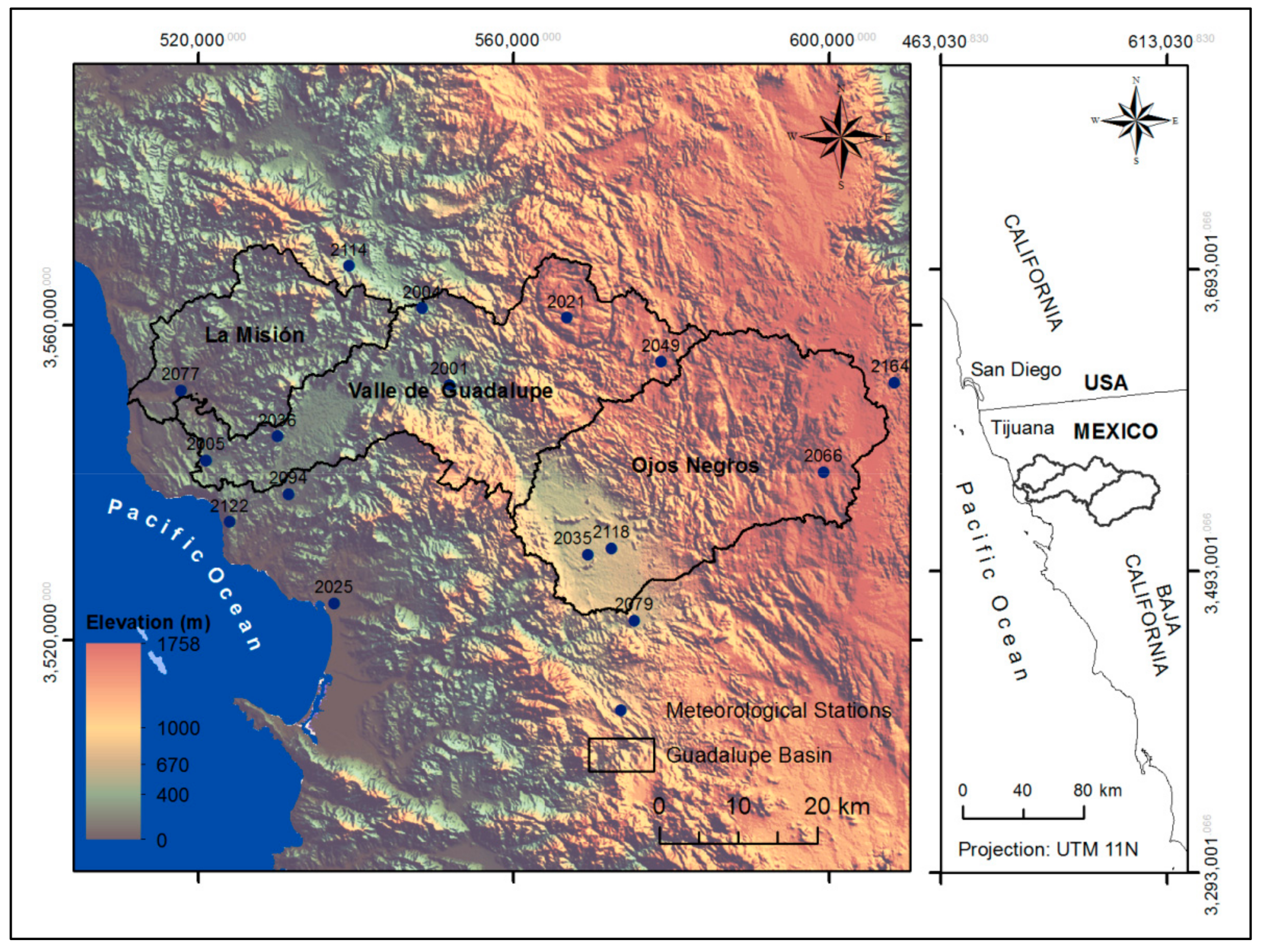
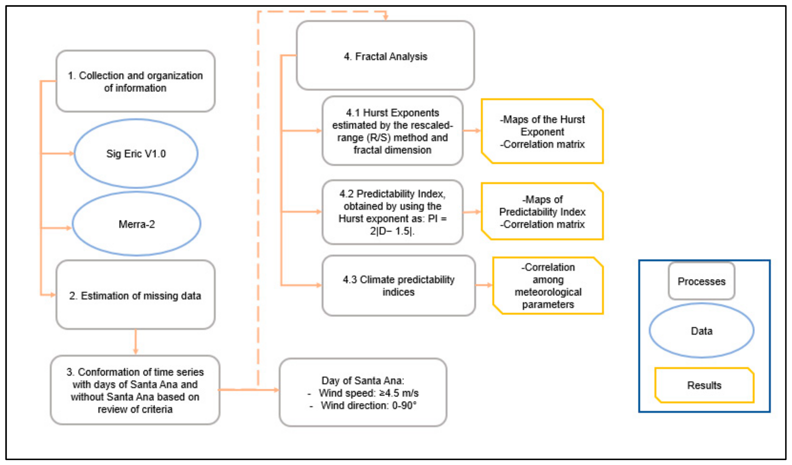
3. Materials and Methods

The study area corresponds to the Guadalupe River basin, located in the northern state of Baja California, between latitudes 31°50′ N, 32°16′ N and longitudes 116°54′ W, 115°52′ W. It is a semi-arid area with a Mediterranean climate, with an average annual temperature of approximately 16 °C and average annual rainfall of approximately 254.6 mm. It has an area of 2390 km2 divided into three sub-basins: Ojos Negros located upstream, Valle de Guadalupe in the central part, and the La Misión sub-basin downstream that flows into the Pacific Ocean (Figure 1) [33].
Thiessen polygons were implemented to estimate the climatological stations that had influence within the basin; 8 stations were found within the basin area and 8 between the basin perimeters and limits for a total of 16 stations.
Figure 2 shows the structure of the methodology used for the proposed analysis.

3.1. Databases

Two databases were used from the Rapid Climatological Information Extractor (ERIC) in its web version (SIG ERIC version 1.0). This has information from stations in the CLICOM database and the National Reference Climatic Network. This database only provides information on maximum, minimum, and observed temperature, precipitation, evaporation, electrical storm, hail, and fog. Data are complemented by the web service, the Modern-Era Retrospective analysis for Research and Applications, Version 2 (MERRA-2), which offers time series of temperature, relative humidity, pressure, wind speed, and direction, precipitation, snowfall, depth of snow, and global horizontal irradiation. The analysis period was between 1980 and 2018.
The following is a list of the stations implemented in the analysis and the Hurst exponents for the variables of pressure (P), temperature (T), rainfall (R), relative humidity (H), and wind speed (W) for the 38-year time series.

3.2. Santa Ana

Criteria used to define the Santa Ana winds (SAW) depend on both the impact of interest (e.g., catastrophic wildfires) and location, and/or day time evaluated [34].
Rolinski et al. [34] proposed a classification of the Santa Ana winds time series, based on the great fire potential L F P w and the mean sea-level pressure gradients (MSLP), where the criteria were: L F P w 6 and W S   4.5 m s 10   mph . Then, the Self-Organizing Maps (SOM) were applied to verify that the time series only contained legitimate days of Santa Ana winds; the most frequent climatic patterns of the zones were verified with the SOMs.
As indicated by Raphael [4], some criteria implemented in the past, such as relative humidity, wind speed, and wind direction, were collected to define the Santa Ana winds. If the average wind speed during four intervals in a day was greater than or equal to 20 mph, the wind direction was from the northeast quadrant, and if the relative humidity at 1630 Pacific Standard Time (PST) was less than 40%, it was considered to be a Santa Ana event. Edinger et al. [35] studied seven years of data from Southern California and the occurrence of a Santa Ana event came with a pressure drop of 3 mb, an increase in temperature of 9 °C, winds from the north with speeds greater than 30 mph, and relative humidity of 30% or less.
Raphael [4] analyzed a 33-year series of meteorological maps, with criteria of high pressure over the Great Basin and low pressure off the Southern California coast, and a prevailing wind direction from the northwest quadrant.
Jones et al. [5] studied 28 years of Fire Climate Index (FWI) values, of which dry winds were a component. The criteria to consider a day as a Santa Ana wind event were as follows: (1) the Great Basin or 30% of the Great Basin had positive gradients in pressure at sea level, (2) the Southern California coasts had negative anomalies in pressure at sea level, and (3) winds over the Los Angeles Basin were from the northeast quadrant.
For Zamora et al. [18], the Santa Ana winds are associated with a change in relative humidity with drops of less than 10%, the direction in the northeast quadrant corresponding to 0° to 90°, and speeds greater than or equal to 20 mph (8.9411 m/s).
Navarro-Olache et al. [15] used criteria of relative humidity below 45% and wind speed greater than or equal to 7 m/s, following those proposed by [7]. Álvarez and Carbajal [1], in the values observed in Ensenada, recorded data of a minimum wind speed of 1.08 m/s and a maximum of 17.91 m/s, temperatures between 11.9 and 31.8 °C, and pressure above sea level between 1008.43 and 1017.93 mb.
Dye et al. [10] classified Santa Ana winds associated with a fire with speeds of 5.19 m/s and wind direction of 38.51°, and Santa Ana winds without fires with speeds of 3.96 m/s and wind direction of 33.54°.
A filter was devised to determine on which days a Santa Ana event occurred and on which days it did not. For the selection of the criterion, the concepts previously exposed and those of [1,3,4,13,15,16,25,26] were reviewed.
A criterion for evaluating a Santa Ana event occurrence associated with wind speed was established at ≥4.5 m/s; the value at which the blaze remains from a fire could accelerate its spread in the air [34]. Consequently, days considered with Santa Ana winds are linked to fires; for the wind direction, the criterion was established in winds from the first quadrant [4,5,18]. The days that meet the two previous conditions are considered days on which a Santa Ana event occurred, the days that do not meet these criteria are considered days on which a Santa Ana wind did not occur.

3.3. Rescaled Range (R/S)

The Hurst exponent and fractal dimension were calculated for the series of time, temperature, relative humidity, pressure, wind speed, and precipitation for days on which the Santa Ana event occurred and on which there were no Santa Ana winds, using the Benoit v1.31 program, following the equations described in (1)–(7).

3.4. Predictability Index

The predictability indices of the variables were estimated using the equations presented in Section 2.2: Equation (8) for pressure, (9) for temperature, (10) for precipitation, (11) for relative humidity, and (12) for wind speed. From these, the climatic predictability index for relative humidity, wind speed, and precipitation were obtained. The first two were of interest as they are related to the Santa Ana winds.

3.5. Spatialization

Spatial distribution maps were generated by the inverse distance weighting interpolation technique (IDW), using ArcGIS software for Hurst exponents, fractal dimension, and predictability indices for temperature, pressure, relative humidity, wind speed, and precipitation.

4. Results and Discussion

4.1. Fractal Analysis
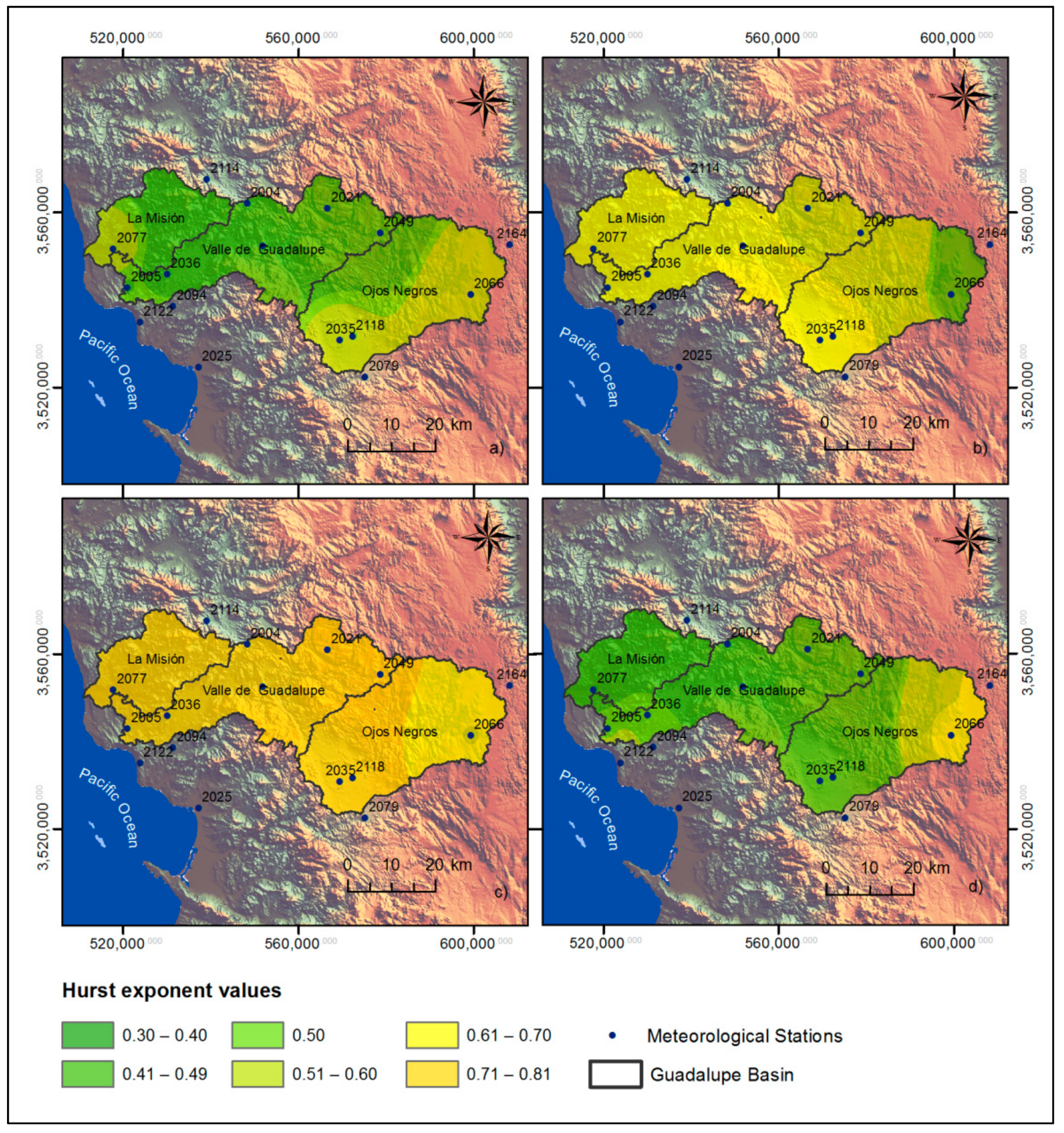
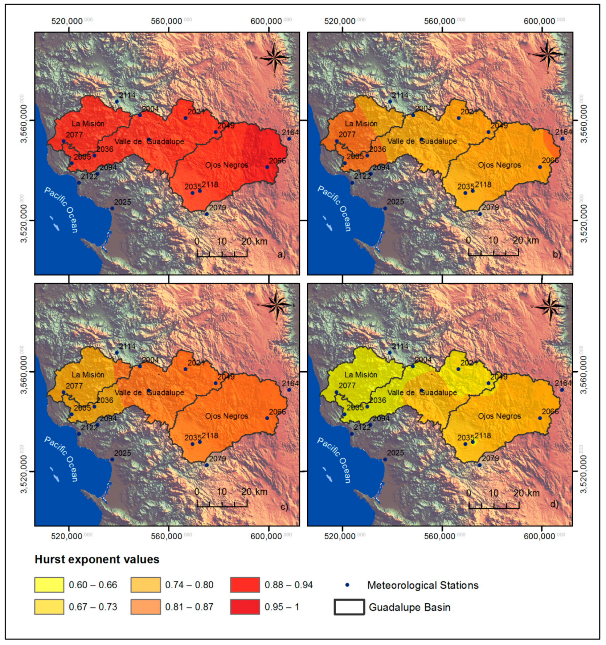
Table 1 shows the weather stations used in the different analyses carried out. The estimated values of the Hurst exponent are also reported for variables of pressure (P), temperature (T), precipitation (R), relative humidity (H), and wind speed (W) from the time series obtained with the databases used.
Values of the Hurst exponent (Table 1) were estimated from the recorded series and without classifying the days on which there was occurrence or non-occurrence of the Santa Ana winds. We aimed to identify the fractal characteristics of the considered study variables and carry out a comparison with the results reported in other research.

Hurst Exponent

Results of the Hurst exponent from the precipitation series show that the variable has persistent behavior by having Hurst exponent values greater than 0.5 t. These results coincide with those reported by [21] in the area under study. These results are also similar to those reported in other places, such as Israel (0.7) [36], Australia (0.6) [37], and Saudi Arabia (059–0.71) [30]. Other works carried out in subtropical and semi-arid climates report values below 0.5, despite having similar conditions to the region under study [38,39,40].
Regarding temperature, values obtained by Mianabadi [41] in Mashad, Iran of 0.6 are similar to ours (0.85–0.96), as they are also persistent. Similarly, for the island of Crete in Greece, the generalized Hurst exponent value of temperature was 0.65 [42]. However, when comparing with Rehman [30], the Hurst exponent values for the temperature in Saudi Arabia are anti-persistent. Regarding wind speed and relative humidity [30], reported average values were 0.64 and 0.61, respectively, similar to those found in the studied region. For the comparison of the pressure Hurst exponent, Rehman [30] found that, in Saudi Arabia, the Hurst exponent took anti-persistent values of 0.2, while those obtained in this research are persistent. This could be due to the fact that the basin’s climate responds to the influences of pressure generated on a large scale in the region and not to local phenomena.
The climate of the Guadalupe basin is generally persistent throughout the year. In some variables, the persistence degree is greater than in others, but it can be generally defined that it has characteristics of a long-term memory when analyzing the temporal structure of the series of precipitation, temperature, pressure, relative humidity, and wind speed. Nonetheless, when breaking down the series to verify the occurrence of the Santa Ana winds phenomenon, it is observed that, during the days when this event does not occur, they maintain the same behavior as the original series. The foregoing confirms that changes in the Hurst exponent values of some variables for the days with Santa Ana winds are linked to the variable of sensitivity to this phenomenon.
Table 2 shows a summary containing the number of days making up the time series established as days with Santa Ana winds, as well as the criteria established to identify said condition in each of the analyzed stations, including: wind speed ≥ 4.5 m/s and wind direction between 0° and 90°. In the first instance, the criterion of relative humidity ≤ 10% was also evaluated, but this criterion was not met on the days when Santa Ana winds had occurred. Relative humidity on those days did not fall to the above limit, so the criteria were reduced only to the speed and direction of the wind. Other research has also ruled out this parameter [1,18].
From the time series resulting from the criteria established above, the Hurst exponents and fractal dimensions were calculated for days with Santa Ana winds and days without Santa Ana winds (Table 3). In this table, T represents temperature, P is pressure, R is rain, H is relative humidity, W is wind speed, and WD is wind direction.
For the data series of days with Santa Ana winds, the Hurst exponent of pressure was greater than 0.5 in most stations, except Sierra De Juárez and Ejido El Porvenir, where it was 0.48 and 0.36, respectively, meaning anti-persistence and indicating that these areas may be affected by local microclimates. The pressure behavior in general is of weak persistence, compared to the strong persistence of the Hurst exponent on days when there are no Santa Ana winds. For the temperature, the Hurst value ranged between 0.43 and 0.59. At the Valle de San Rafael station, the Hurst exponent value was 0.5, while at the Ejido Porvenir, Boquilla, Santa Rosa de La Misión, and El Farito stations, the estimated value of the Hurst exponent was 0.49. This behavior was also found in the Agua Caliente, El Pinal, Olivares Mexicanos, San Juan De Dios Norte, and Ejido Carmen Serdán stations. Generally, for temperature, a change in the Hurst exponent value can be noticed between one condition and the other, i.e., on days without Santa Ana winds, it is very persistent, but when this phenomenon occurs, the temperature becomes anti-persistent in many zones. This could be a consequence of large fluctuations in temperature at these times of the year, becoming random in a certain places, as already mentioned.
Regarding precipitation data recorded on the days with Santa Ana winds, the Hurst exponent could not be estimated for all weather stations because there were not enough data to use the rescaled range analysis. In the cases where it was possible to estimate Hurst exponent values for precipitation, the analyses resulted in values greater than 0.5, maintaining persistent characteristics. Nonetheless, at the Real del Castillo Viejo and La Misión stations, values obtained were 0.31 and 0.23, respectively. For the Alamar station, random behavior was determined for days with Santa Ana winds.
For the series of the relative humidity variable, results yielded Hurst exponent values greater than 0.5 in all the weather stations analyzed. These persistence conditions are maintained when the Santa Ana winds do and do not occur.
In the case of the wind speed series, Hurst exponent values denote a trend for the variable to have an anti-persistent behavior because the values are less than 0.5. However, in the Sierra de Juárez and Ejido El Porvenir stations, values of 0.63 were estimated, and for the Ensenada and Real del Castillo Viejo stations, values of 0.54 and 0.55 were, respectively, estimated. Based on these results, it could be said that wind speed and temperature are regulated by the winds from the Great Basin and the pressure gradients generated during this time, as opposed to pressure and relative humidity, regardless of occurrence. The condition of the Santa Ana winds conserves the persistence in the series even to a lesser degree. Relative humidity does not reflect the changes in the value of the Hurst exponent that would be expected for the time of Santa Ana, i.e., the values of the Hurst exponent did not remain in the same range, but instead became anti-persistent values or random in said season, as occurs with other variables such as wind speed and temperature, where the behavior of the Hurst exponent is not the same for the two analysis conditions.
This situation may be due to what was mentioned above about the records, which, in most stations, did not have relative humidity values ≤ 10%, as suggested by the classification criteria. In some stations where it was found that the aforementioned criteria were met, they did not coincide with the months of the Santa Ana season, but rather with the time when this type of wind was not expected to occur. Furthermore, many of these criteria are based on analyses carried out in the United States, and the phenomenon, when it reaches the Baja California region, does not enter with the same intensity and varies according to the topographic characteristics of the area. This was evidenced in the correlation matrices and variables’ spatialization maps, where not all the basin has the same behavior for the variables analyzed, as will be thoroughly examined in Section 4.3.
Furthermore, the Hurst exponent of the wind direction was estimated, determining values less than 0.5 for most of the stations. Only in El Alamar, the Hurst value was 0.53. Random conditions were present at the Ojos Negros and Valle De San Rafael stations. In the Sierra de Juárez station, the anti-persistence was stronger than in the other stations, with a value of 0.18. These results were for the condition of days with Santa Ana winds, while, for days without Santa Ana winds, the wind direction was persistent.
This is due to the fact that when there are Santa Ana Winds, the climate is altered. As relative humidity decreases, wind speed increases. The direction of these winds is only from the first quadrant, and temperatures can or cannot fall. This invariance in the time series scale is affected by a regional phenomenon called the Santa Ana winds, since, when segmenting the complete vector into two seasons, changes are observed, as evidenced in the previous analyses. In the Hurst values of the days when there are no Santa Ana winds, it is observed that the occurrence of pressure, temperature, precipitation, relative humidity, wind speed, and even wind direction is influenced by many regional and/or large-scale weather systems, e.g., Tatli [43] determined high persistence values of the Hurst exponent, for which it was affirmed that many regional and/or large-scale climatic systems influenced the occurrence of droughts over Turkey. If some small-scale atmospheric systems were effective in the formation of droughts, then at least some values of H < 0.5 should be obtained, a result that did not occur.
For the Hurst exponents on days with Santa Ana winds, it is observed that this regional phenomenon modifies the climatic dynamics of the basin, altering the variables involved in it with different intensities.

4.2. Predictability Index

Table 4 shows the values obtained for the predictability indices of pressure, temperature, precipitation, relative humidity, wind speed, and wind direction for the days with and without Santa Ana winds.
If one of the indices from the table above is close to zero, the process approaches a Brownian motion and is therefore unpredictable. If this is close to 1, the process is very predictable.
Regarding predictability indices in general, when there are Santa Ana winds, the variables of pressure, temperature, wind speed, and wind direction become unpredictable, while, when there are no Santa Ana winds, they are predictable. Relative humidity also becomes less predictable, as evidenced in Table 4, becoming unpredictable in certain stations, such as Sierra Juárez and Ejido el Porvenir. Additionally, it is observed that, for the precipitation predictability index at the Ignacio Zaragoza Belén, Boquilla Santa Rosa de La Misión, Ensenada, El Farito, and La Misión stations, they have values greater than 0.5, i.e., their predictability is closer to 1, meaning that they are quite predictable, in contrast to the Ojos Negros, El Alamar, Valle De San Rafael, El Pinal, Real del Castillo Viejo, and Ejido Carmen Serdán stations, where the index has values closer to 0, meaning that the precipitation variable is unpredictable.

4.2.1. Climatic Predictability Index

For the climatic predictability indices of precipitation, relative humidity, and wind speed, an analysis was carried out to evaluate how temperature and pressure impacted the aforementioned variables. Table 5 shows the interaction between these variables when a Santa Ana event occurs and Table 6 for days without Santa Ana winds. The * indicates stations where the Hurst exponent, the fractal dimension, and, therefore, the climatic predictability indices of precipitation could not be estimated because the precipitation series did not have the minimum data necessary to be able to perform the analyses.
For the analysis of windy days with Santa Ana and without Santa Ana winds, the value of 0.4 is established as the limit or the value where the series begins to be considered predictable, as proposed by Li et al. [31]. It was observed that temperature and pressure control or impact the relative humidity parameter in the Sierra de Juárez and Ejido El Porvenir stations, i.e., the pressure predictability index and the temperature predictability index affect or vary in the same measure, but they are not predictable. This happens when there are Santa Ana days. Otherwise, it happens with the days where there is no Santa Ana event, where the relative humidity is very predictable in most stations and the predictability index of the relative humidity is controlled by the predictability index of temperature and pressure. In other words, the relationship between temperature, pressure, and relative humidity is only maintained in the two stations already mentioned for the two cases presented.
Wind speed is unpredictable whether it is the Santa Ana or non-Santa Ana season. However, for the Santa Ana season, both the pressure, temperature, and wind speed become unpredictable and exhibit an apparent correlation. This is a logical observation since these variables are characteristics of the Santa Ana phenomenon. Otherwise, it happens in the non-Santa Ana period, where the predictability indices of pressure and temperature are very predictable but the predictability index of wind speed is not, so they are not closely related, reflecting that speed is an independent variable from the others in conditions where it is not associated with a climatic phenomenon.
In the case of rain, despite not being a relevant variable associated with the Santa Ana phenomenon, on days without Santa Ana winds, it shows a relationship with temperature and pressure, as the three values are predictable. For days with Santa Ana winds, this relationship is only maintained in five of the evaluated stations.
The previous analysis was complemented by a correlation matrix developed for conditions of the occurrence and non-occurrence of days with Santa Ana winds for the predictability indices of the variables under study, as shown in Figure 3, in which some of the relationships shown by the fractal analysis of the same are verified. The analysis was complemented by the spatialization of the predictability indices of the variables used, which will be discussed in detail in the next subsection.

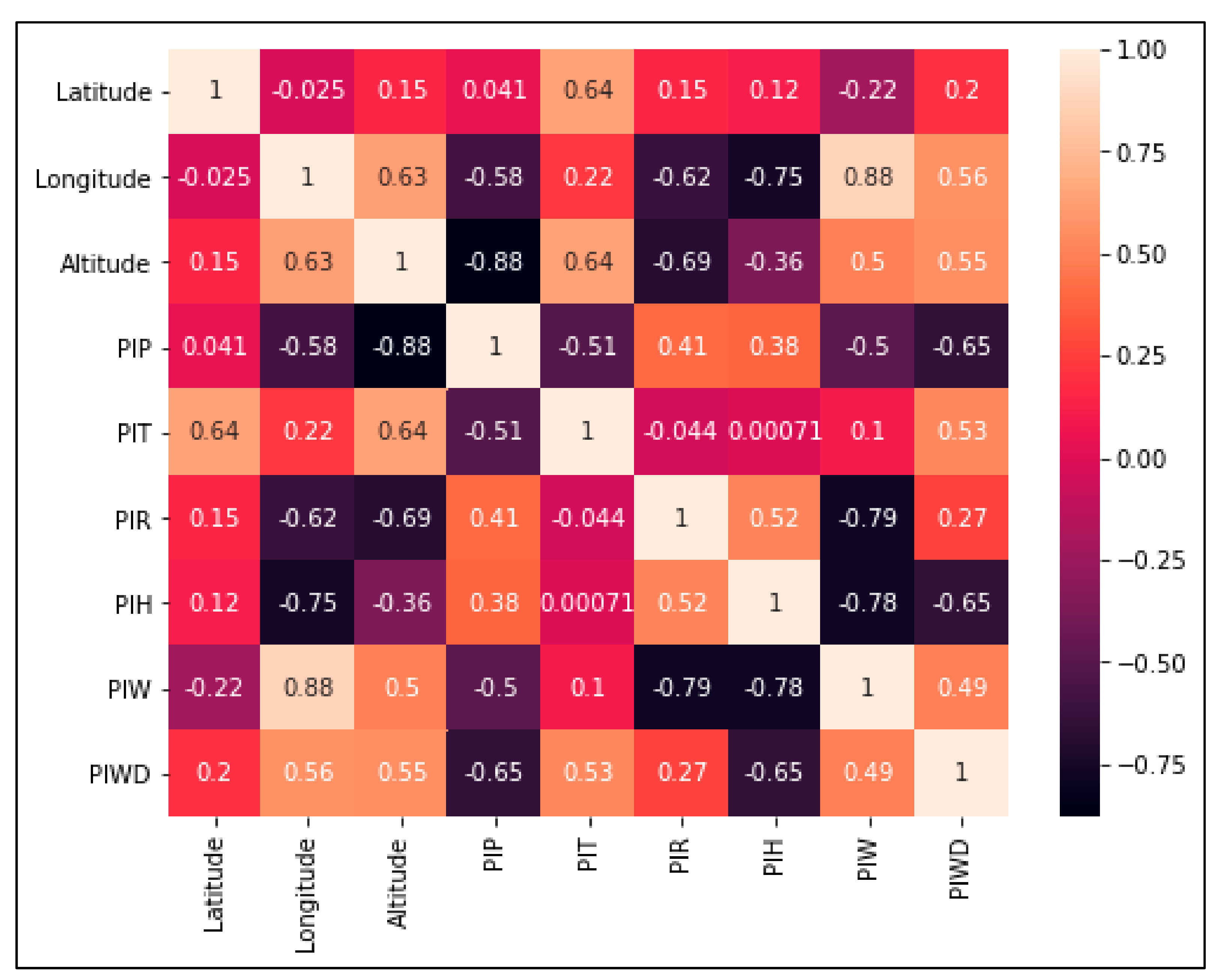
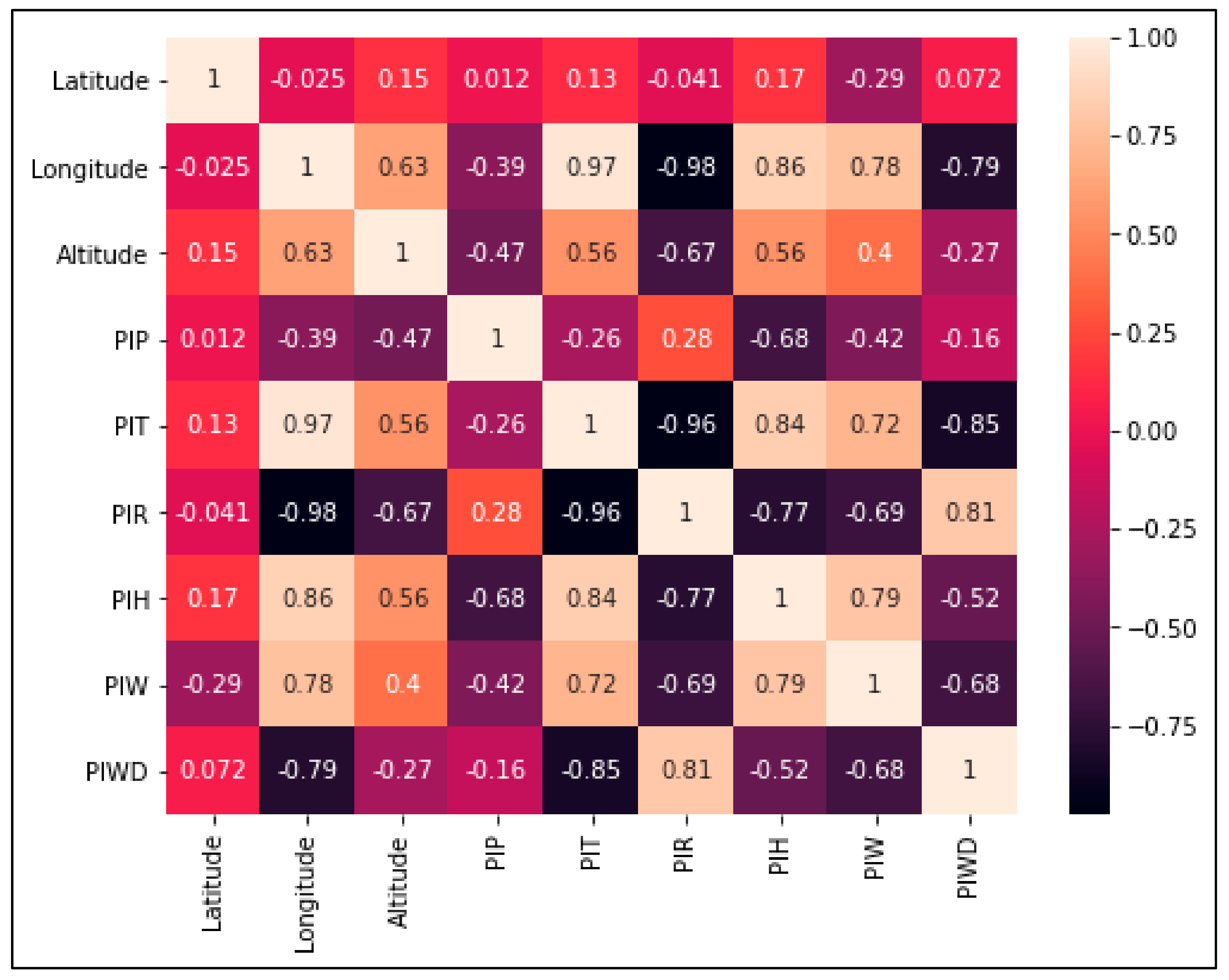
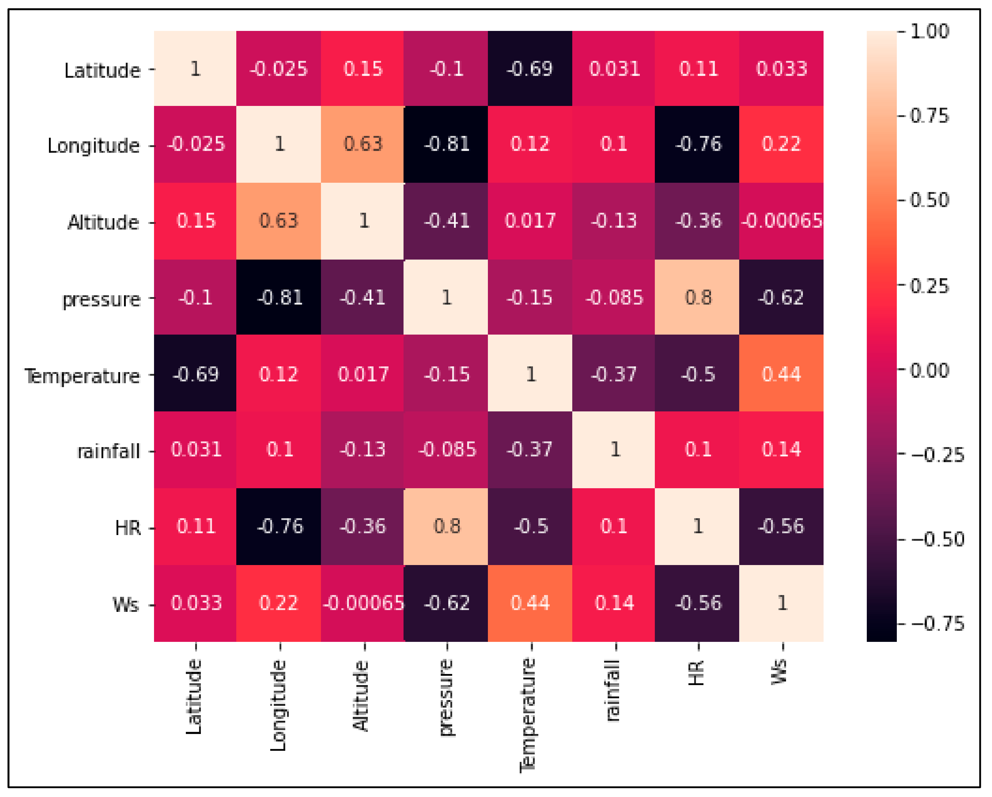
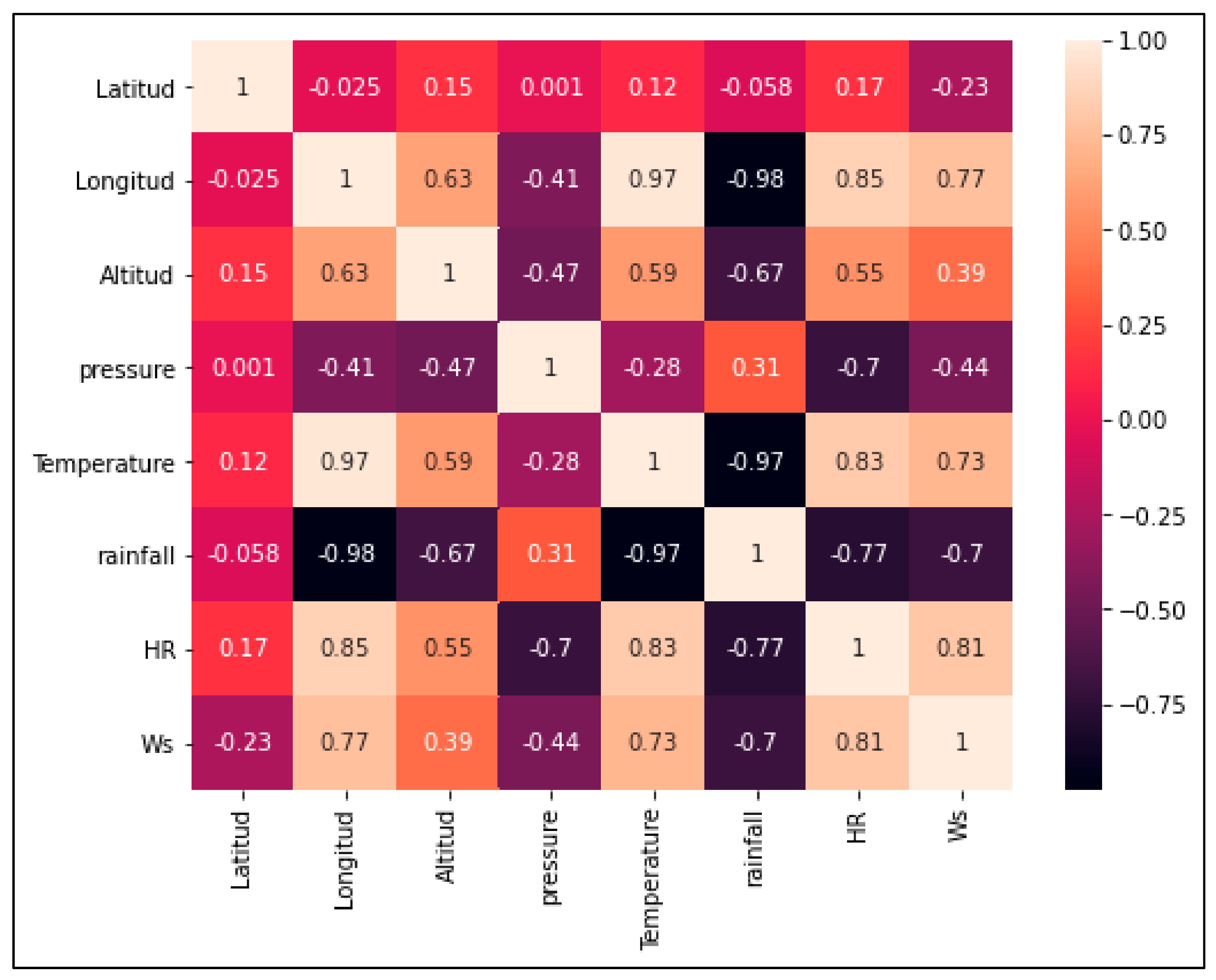
4.2.2. Correlation Matrix Predictability Index

Two correlation matrices were generated for the two study cases, where light colors correspond to positive correlations and dark colors to negative correlations. The Pearson’s method was used because it can quantify the linear relationship between stationary time series, such as those studied [44,45], which is observed in the correlations obtained for the two scenarios.
The ranges used to measure correlation degree are shown in Table 7.
In the previous correlation matrix, altitude shows a significant negative correlation with P I P and I P H for days with Santa Ana winds, with P I T and P I W being positive but moderate. As for the P I P , with respect to P I R , it is weak, and with the P I T , it is null, confirming the relationship shown by the P I C R as shown in Figure 4. A similar case occurs for the relative humidity, reflecting what is shown by the P I C H , leaving open the possibility that the weather stations where there is a relationship between the predictability indices of relative humidity, temperature, and pressure, and between precipitation, temperature, and pressure, depends on other factors, such as the station’s geographical location and altitude. For P I W , the relationship is moderate with respect to P I P and is negative, while, with P I T , it is very weak.
The altitude for Santa’s windless days shows a weak correlation with P I P and moderate with P I R n, but negative, while, with P I T and P I H , it is moderate but positive. As for P I P with P I R , they exhibit a weak but positive and perfect but negative relationship with P I T T. The P I H and the P I T have a significant and positive relationship, while, with the P I P , it is negative and moderate. The P I W has a negative and weak correlation with the P I P , while, with P I T , it is positive and significant.

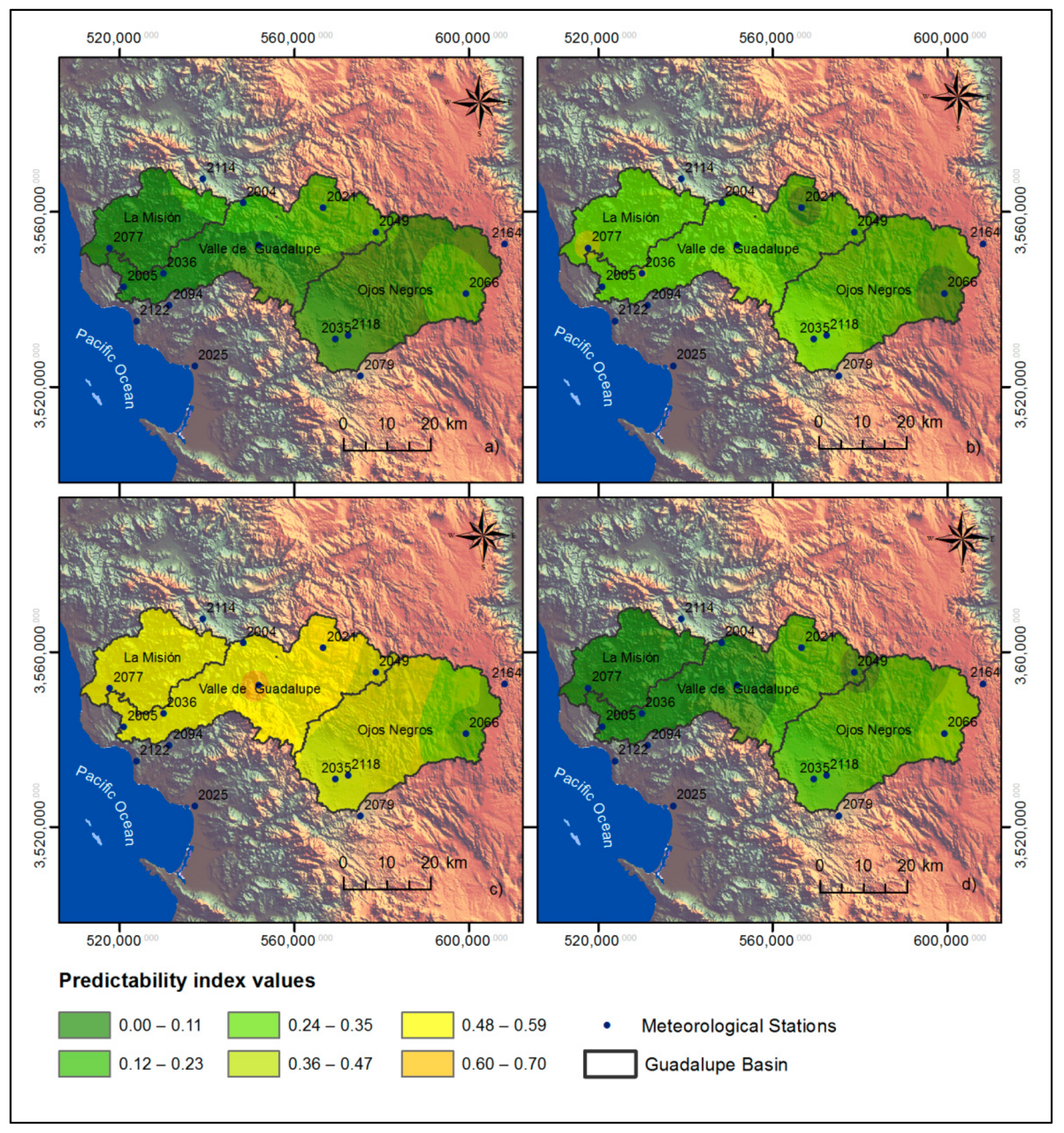
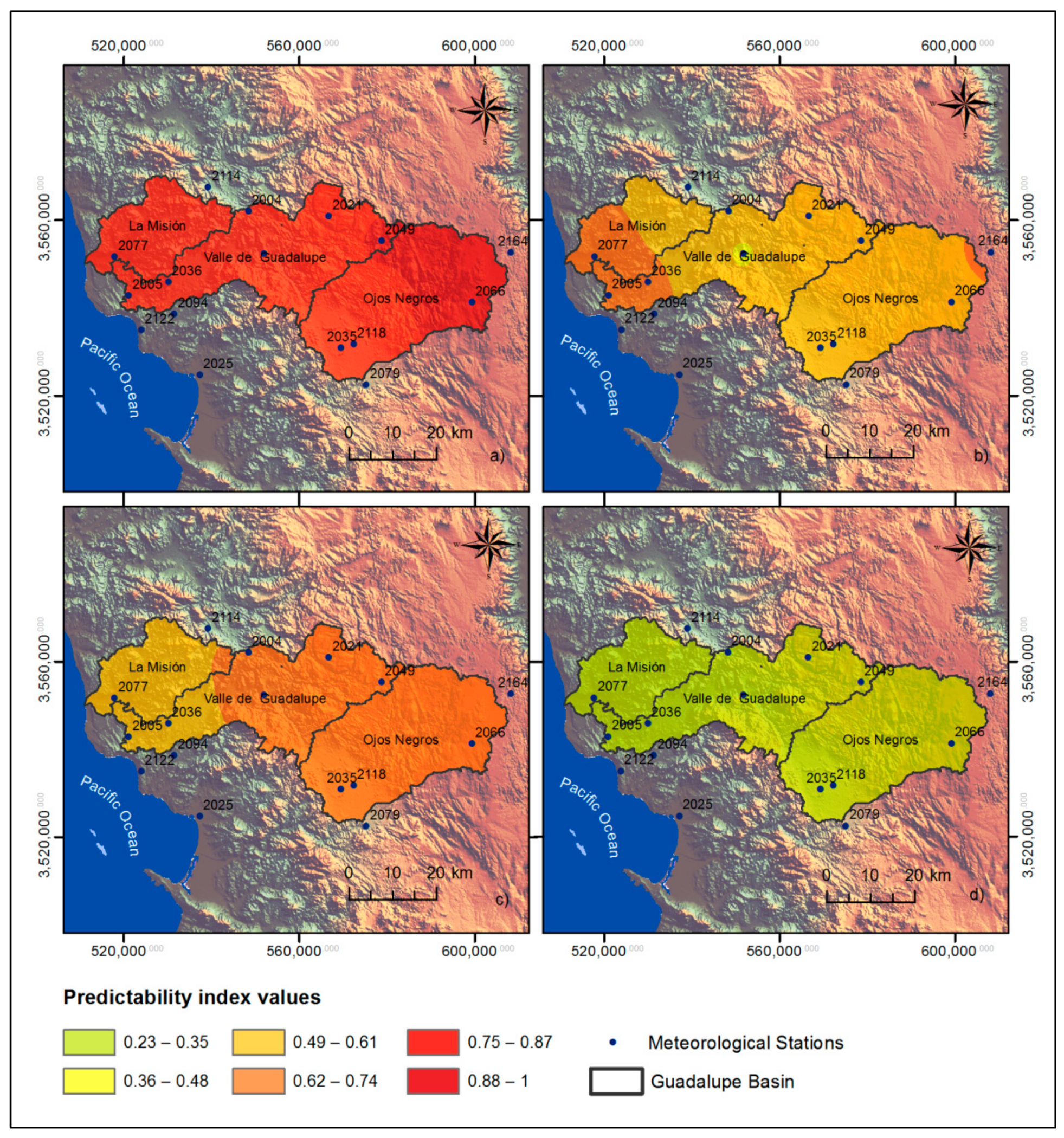
4.3. Geospatialization

Below are the maps obtained from the spatialization of the Hurst exponent and the predictability index for the variables of temperature, pressure, relative humidity, and wind speed for the conditions with Santa Ana winds and in the absence of Santa Ana winds.
To complement the analyses from the geospatialization of the Hurst exponents of the climatic variables under study, a correlation analysis was carried out for the two seasons analyzed, i.e., for the series that represent the Santa Ana winds season (Figure 5) and for the series that do not involve this condition (Figure 6). In these matrices, when referring to pressure, we refer to the exponent values of Hurst of the pressure; the same goes for temperature, relative humidity (RH), rainfall (precipitation), and Ws, the Hurst exponent of the wind speed.
In Figure 7, maps of the Hurst exponent are shown for the time series made up of days with Santa Ana winds. In this figure, it is observed that the temperature variable presents the lowest Hurst values and it tends to have an anti-persistent behavior throughout the basin. The El Pinal station is located in one of the highest areas (masl) of the basin and there are low values in it, in contrast to the Sierra Juárez station, the highest point (masl) of the basin, but the Hurst exponents estimated here are higher. From the correlation matrix in Figure 5, it is determined that the altitude has no correlation with the Hurst values for the temperature series. For pressure, the highest values of the Hurst exponent occur in the lower part of the basin; there is an inverse correlation between altitude and longitude. This would explain why, in the analysis, the Sierra Juárez and Ejido Porvenir stations show the lowest values in the basin. In the case of relative humidity, the opposite happens with pressure: the lowest values are found in the Sierra de Juárez station, being the place with the highest altitude in the basin. The highest Hurst values for this variable are found in low-altitude areas and in the Guadalupe Valley sub-basin.
For wind speed, the Sierra de Juárez station is the one that presents the highest value of the Hurst exponent; however, the El Pinal and San Juan de Dios Norte stations present low Hurst values, despite being located in a high area of the basin. Therefore, it can be said that there is no clear relationship between wind speed and altitude.
In Figure 8, maps of the Hurst exponent are presented for the time series made up of days without Santa Ana winds. As shown in the matrix in Figure 6, temperature has a positive relationship with altitude. In the highest area, where the Sierra de Juárez station is located, the highest values of the Hurst exponent are shown; likewise, the lowest values of said exponent are found in the lowest area of the basin, corresponding to the Mission sub-basin. The temperature series is persistent, with high values close to 1. The analyses of the correlation matrix in Figure 6 also show that the temperature has a significant correlation with the relative humidity variable. In the case of the exponent values for pressure, the highest values occur in the lower parts of the basin or at lower altitudes (masl), i.e., there is a weak and inverse correlation between these parameters; in the same way, it maintains this relationship with the length. For relative humidity, the relationship is positive with respect to altitude, i.e., the highest values correspond to the highest areas of the basin. This relationship is the same for relative humidity with longitude. In the case of wind speed, the correlation with altitude is weak and positive, while the relationship with longitude is positive and significant, which can explain the high values in the eastern part of the basin.
From the above, we can affirm that the Santa Ana winds modify the relationships between the variables and the geographical characteristics of the seasons, i.e., during the normal days of the year, the pressure has an inverse relationship with longitude and altitude, but the longitude increases when there are Santa Ana winds. For relative humidity, it is found that the relationship becomes inverse during the Santa Ana season; in the case of temperature and wind speed, the degrees of relationship that existed at the time without Santa Ana winds fell until they were null or very weak, which is evident since these variables are the ones that reflect the largest changes from one season to another.
From Figure 9, for temperature, it is observed that there is a positive and moderate relationship with respect to altitude. It is observed that the highest values correspond to the Sierra Juárez, El Pinal, and San Juan de Dios Norte stations. For the values of the pressure predictability indices, there is an inverse correlation with altitude, and the lowest values are found in the stations mentioned above. Regarding the predictability index of relative humidity, the relationship with altitude is also inverse but weak; the map shows that the highest values are in the middle basin, corresponding to the Valle de Guadalupe sub-basin; meanwhile, the relationship between the length and the predictability index of the relative humidity is also inverse but significant. The highest values of the Hurst exponent when analyzing the wind speed series are presented in the stations of Sierra Juárez and Ejido el Porvenir. The relationship between wind speed and altitude is generally moderate and positive, as it is with longitude, this being more a significant relationship. Thus, when reviewing the correlations of pressure and temperature with respect to relative humidity, from the correlation matrix (Figure 3) and from the predictability analysis (Table 5), it is found that the relationship is null with temperature and weak with pressure in the stations in which the influence of said variables is presented, due to their geographic location parameters. Meanwhile, for wind speed, the relationship with temperature is weak and positive. In the case of pressure, it is negative and moderate.
In Figure 4 and Figure 10 and Table 6, temperature shows a positive relationship with altitude, where the highest values of the predictability index are found in the areas where the Sierra de Juárez and Ejido el Porvenir stations are located. It should be noted that the Ejido el Porvenir station is located at a lower elevation than the Sierra de Juárez station; nonetheless, they present similar values for the predictability index. This may be due to the high correlation between longitude and temperature. For pressure, there is a weak and inverse relationship with altitude, evidenced in that the highest values of the pressure predictability index are in the La Misión, Boquilla de Santa Rosa de La Misión, and Ejido el Porvenir stations. The lowest values of the pressure predictability index are found in the upper parts of the basin, such as the El Pinal station. From the correlation matrix (Figure 3), it can be seen that, for relative humidity, the relationship is moderate with respect to altitude, and positive, as observed in Figure 9, where the lowest ranges correspond to the lower part of the basin and the highest to the highest part of the basin. For wind speed, the relationship with altitude is positive but weak, although predictability is lower in the Mission and higher in Sierra de Juárez. Agua Caliente, a station with an intermediate height, has a predictability equal to that of Sierra de Juárez.

5. Conclusions

The following conclusions were established from the fractal analysis by estimating the Hurst exponent and the climatic predictability indices.
The rescaled range method was adequate to evaluate the fractality of the time series that represent the conditions of occurrence of the Santa Ana winds and for the series that represent the days on which said phenomenon does not occur. From the estimation of the Hurst exponent, it was possible to characterize the time series of the variables of temperature, precipitation, pressure, relative humidity, and wind speed in terms of the characteristics of persistence, anti-persistence, or randomness.
When there are phenomena that alter the climate of an area, such as the Santa Ana winds, the interaction and behavior of the climatic variables in its environment can be modified regarding the conditions that occur or are normally recorded, e.g., when performing the fractal analysis of a specific variable, we can have predictable characteristics and persistent behaviors; nonetheless, this can change when performing the same analysis in periods of occurrence of Santa Ana events, as is the case of wind speed, which, during periods with Santa Ana events, exhibits anti-persistent behavior in most seasons but persistent and predictable during the months when there are no Santa Ana events.
This also happens for the temperature, or, in more specific cases, such as the Ejido el Porvenir and Sierra de Juárez stations, where the pressure changes from being persistent on normal days to being anti-persistent for days with Santa Ana winds, or the predictability of wind speed in Sierra Juárez and Ejido el Porvenir, where the wind behavior is unpredictable and independent of the season, whether or not there is a Santa Ana wind event. This leads us to conclude that the index can be used as a discriminant in determining which stations can be selected for use in developing regional climate models.
The analysis of the correlation matrices allows us to understand the relationships of the climate dynamics in an area and how these correlations can change in relation to different seasons, e.g., the relationship between the predictability index of relative humidity and speed remains independent of the segmentation analysis (whether Santa Ana condition exists or not) but relative humidity and altitude change from a positive relationship in normal conditions to an inverse relationship on days with Santa Ana winds.
It is recommended to conduct studies in which the criterion of relative humidity < 10% is utilized for the identification of the condition of the Santa Ana winds.
Finally, this type of study contributes to understanding the regional dynamics of the Guadalupe basin and to establishing a basis for the development of models that allow forecasting of the days on which the Santa Ana winds occur in said basin in order to mitigate the negative consequences that can be generated, e.g., fires and droughts.

Author Contributions

Conceptualization, Y.S.-U., A.A.L.-L., D.-L.F., M.L.-L., E.G.-B., L.M.-A., J.P.M.-B., J.F.R.L. and A.L.-R.; methodology, Y.S.-U., A.A.L.-L., E.G.-B., L.M.-A., J.P.M.-B., J.F.R.L. and A.L.-R.; formal analysis, Y.S.-U., A.A.L.-L., E.G.-B., L.M.-A., J.P.M.-B., J.F.R.L. and A.L.-R.; investigation, Y.S.-U., A.A.L.-L., E.G.-B., L.M.-A., J.P.M.-B., J.F.R.L. and A.L.-R.; resources, Y.S.-U., A.A.L.-L., E.G.-B., L.M.-A., J.P.M.-B., J.F.R.L. and A.L.-R.; writing—original draft preparation, Y.S.-U., A.A.L.-L., E.G.-B., L.M.-A., J.P.M.-B., J.F.R.L. and A.L.-R.; writing—review and editing, Y.S.-U., A.A.L.-L., E.G.-B., L.M.-A., J.P.M.-B., J.F.R.L. and A.L.-R.; funding acquisition, Y.S.-U., A.A.L.-L., E.G.-B., L.M.-A., J.P.M.-B., J.F.R.L. and A.L.-R. All authors have read and agreed to the published version of the manuscript.

Funding

This research was funded by HIDRUS S.A de C.V, Grupo HIDRUS S.A.S and Universidad Pontificia Bolivariana Campus Montería; the APC was funded by HIDRUS S.A de C.V and Grupo HIDRUS S.A.S.

Institutional Review Board Statement

Not applicable. This study did not require ethical approval.

Informed Consent Statement

Not applicable. This study did not involve humans.

Data Availability Statement

Not applicable. This study did not report any data.

Conflicts of Interest

The authors declare no conflict of interest.

References

  1. Álvarez, C.A.; Carbajal, N. Regions of influence and environmental effects of Santa Ana wind event. Air Qual. Atmos. Health 2019, 12, 1019–1034. [Google Scholar] [CrossRef]
  2. Glickman, T.S.; Zenk, W. Glossary of Meteorology; Ametican Meteorogical Society: Boston, MA, USA, 2021. [Google Scholar]
  3. Schwarz, L.; Malig, B.; Guzman-Morales, J.; Guirguis, K.; Ilango, S.D.; Sheridan, P.; Gershunov, A.; Basu, R.; Benmarhnia, T. The health burden of fall, winter and spring extreme heat events in Southern California and contribution of Santa Ana Winds. Environ. Res. Lett. 2020, 15, 054017. [Google Scholar] [CrossRef]
  4. Raphael, M.N. The Santa Ana Winds of California. Earth Interact. 2003, 7, 1–13. [Google Scholar] [CrossRef]
  5. Jones, C.; Fujioka, F.; Carvalho, L.M.V. Forecast skill of synoptic conditions associated with Santa Ana winds in Southern California. Mon. Weather Rev. 2010, 138, 4528–4541. [Google Scholar] [CrossRef] [Green Version]
  6. Abatzoglou, J.T.; Barbero, R.; Nauslar, N.J. Diagnosing santa ana winds in Southern California with synoptic-scale analysis. Weather Forecast. 2013, 28, 704–710. [Google Scholar] [CrossRef]
  7. Guzman-Morales, J.; Gershunov, A.; Theiss, J.; Li, H.; Cayan, D. Santa Ana Winds of Southern California: Their climatology, extremes, and behavior spanning six and a half decades. Geophys. Res. Lett. 2016, 43, 2827–2834. [Google Scholar] [CrossRef] [Green Version]
  8. Conil, S.; Hall, A. Local regimes of atmospheric variability: A case study of Southern California. J. Clim. 2006, 19, 4308–4324. [Google Scholar] [CrossRef]
  9. Hughes, M.; Hall, A. Local and synoptic mechanisms causing Southern California’s Santa Ana winds. Clim. Dyn. 2010, 34, 847–857. [Google Scholar] [CrossRef] [Green Version]
  10. Dye, A.W.; Kim, J.B.; Riley, K.L. Spatial heterogeneity of winds during Santa Ana and non-Santa Ana wildfires in Southern California with implications for fire risk modeling. Heliyon 2020, 6, e04159. [Google Scholar] [CrossRef]
  11. Rolinski, T.; Capps, S.B.; Fovell, R.G.; Cao, Y.; D’Agostino, B.J.; Vanderburg, S. The Santa Ana wildfire threat index: Methodology and operational implementation. Weather Forecast. 2016, 31, 1881–1897. [Google Scholar] [CrossRef]
  12. Billmire, M.; French, N.H.F.; Loboda, T.; Owen, R.C.; Tyner, M. Santa Ana winds and predictors of wildfire progression in southern California. Int. J. Wildland Fire 2014, 23, 1119–1129. [Google Scholar] [CrossRef]
  13. Cao, Y. The Santa Ana Winds of Southern California in the Context of Fire Weather. Ph.D. Thesis, University of California, Los Angeles, CA, USA, 2015. [Google Scholar]
  14. Cao, Y.; Fovell, R.G. Downslope windstorms of San Diego County. Part I: A case study. Mon. Weather Rev. 2016, 144, 529–552. [Google Scholar] [CrossRef]
  15. Navarro-Olache, L.F.; Castro, R.; Durazo, R.; Hernández-Walls, R.; Mejía-Trejo, A.; Flores-Vidal, X.; Flores-Morales, A.L. Influence of Santa Ana winds on the surface circulation of Todos Santos Bay, Baja California, Mexico. Atmósfera 2021, 34, 97–109. [Google Scholar] [CrossRef] [Green Version]
  16. Trasviña, A.; Ortiz-Figueroa, M.; Herrera, H.; Cosío, M.A.; González, E. “Santa Ana” winds and upwelling filaments off Northern Baja California. Dyn. Atmos. Ocean. 2003, 37, 113–129. [Google Scholar] [CrossRef]
  17. Castro, R.; Parés-Sierra, A.; Marinone, S. Evolution and extension of the Santa Ana winds of February 2002 over the ocean, off California and the Baja California Peninsula. Cienc. Mar. 2003, 29, 275–281. [Google Scholar] [CrossRef] [Green Version]
  18. Zamora, M.; Lambert, A.; Montero, G. Effect of some meteorological phenomena on the wind potential of Baja California. Energy Procedia 2014, 57, 1327–1336. [Google Scholar] [CrossRef] [Green Version]
  19. Sosa-Avalos, R.; Gaxiola-Castro, G.; Durazo, R.; Greg-Mitchell, B. Effect of Santa Ana winds on bio-optical properties off Baja California. Cienc. Mar. 2005, 31, 339–348. [Google Scholar] [CrossRef] [Green Version]
  20. Millán, H.; Kalauzi, A.; Cukic, M.; Biondi, R. Nonlinear dynamics of meteorological variables: Multifractality and chaotic invariants in daily records from Pastaza, Ecuador. Theor. Appl. Climatol. 2010, 102, 75–85. [Google Scholar] [CrossRef]
  21. López-Lambraño, A.A.; Fuentes, C.; López-Ramos, A.A.; Mata-Ramírez, J.; López-Lambraño, M. Spatial and temporal Hurst exponent variability of rainfall series based on the climatological distribution in a semiarid region in Mexico. Atmosfera 2018, 31, 199–219. [Google Scholar] [CrossRef]
  22. Caldeira, R.; Fernández, I.; Pacheco, J.M. On NAO’s predictability through the DFA method. Meteorol. Atmos. Phys. 2007, 96, 221–227. [Google Scholar] [CrossRef]
  23. Maruyama, F.; Kai, K.; Morimoto, H. Wavelet-based multifractal analysis on a time series of solar activity and PDO climate index. Adv. Space Res. 2017, 60, 1363–1372. [Google Scholar] [CrossRef]
  24. Diodato, N.; de Guenni, L.B.; Garcia, M.; Bellocchi, G. Decadal oscillation in the predictability of Palmer Drought Severity Index in California. Climate 2019, 7, 6. [Google Scholar] [CrossRef] [Green Version]
  25. da Silva, H.S.; Silva, J.R.S.; Stosic, T. Multifractal analysis of air temperature in Brazil. Phys. A Stat. Mech. Its Appl. 2020, 549, 124333. [Google Scholar] [CrossRef]
  26. Harrouni, S.; Guessoum, A. Using fractal dimension to quantify long-range persistence in global solar radiation. Chaos Solitons Fractals 2009, 41, 1520–1530. [Google Scholar] [CrossRef]
  27. López-Lambraño, A.; Carrillo-Yee, E.; Fuentes, C.; López-Ramos, A.; López-Lambraño, M. Una revisión de los métodos para estimar el exponente de Hurst y la dimensión fractal en series de precipitación y temperatura. Rev. Mex. Fis. 2017, 63, 244–267. [Google Scholar]
  28. Rehman, S.; Siddiqi, A.H. Wavelet based correlation coefficient of time series of Saudi Meteorological Data. Chaos Solitons Fractals 2009, 39, 1764–1789. [Google Scholar] [CrossRef]
  29. Rangarajan, G.; Sant, D.A. A climate predictability index and its applications. Geophys. Res. Lett. 1997, 24, 1239–1242. [Google Scholar] [CrossRef]
  30. Rehman, S. Study of Saudi Arabian climatic conditions using Hurst exponent and climatic predictability index. Chaos Solitons Fractals 2009, 39, 499–509. [Google Scholar] [CrossRef]
  31. Li, M.; Xia, J.; Meng, D.J. DFA based predictability indices analysis of climatic dynamics in Beijing area, China. Adv. Mater. Res. 2012, 382, 60–64. [Google Scholar] [CrossRef]
  32. Ryu, S.; Song, J.J.; Kim, Y.; Jung, S.H.; Do, Y.; Lee, G.W. Spatial Interpolation of Gauge Measured Rainfall Using Compressed Sensing. Asia-Pac. J. Atmos. Sci. 2021, 57, 331–345. [Google Scholar] [CrossRef] [Green Version]
  33. Martínez-Acosta, L.; Medrano-Barboza, J.P.; López-Ramos, Á.; Remolina López, J.; López-Lambraño, A.A. SARIMA Approach to Generating Synthetic Monthly Rainfall in the Sin ú River Watershed in Colombia. Atmosphere 2020, 11, 602. [Google Scholar] [CrossRef]
  34. Rolinski, T.; Capps, S.B.; Zhuang, W. Santa Ana winds: A descriptive climatology. Weather Forecast. 2019, 34, 257–275. [Google Scholar] [CrossRef]
  35. Edinger, J.G.; Helvey, R.A.; Baumhefner, D. Surface Wind Patterns in the Los Angeles Basing during “Santa Ana” Conditions; University of California: Los Angeles, CA, USA, 1964; pp. 1–73. [Google Scholar]
  36. Broday, D.M. Studying the time scale dependence of environmental variables predictability using fractal analysis. Environ. Sci. Technol. 2010, 44, 4629–4634. [Google Scholar] [CrossRef] [PubMed]
  37. Korvin, G.; Boyd, D.M.; O’Dowd, R. Fractal characterization of the South Australian gravity station network. Geophys. J. Int. 1990, 100, 535–539. [Google Scholar] [CrossRef] [Green Version]
  38. Peñate, I.; Martín-González, J.M.; Rodríguez, G.; Cianca, A. Scaling properties of rainfall and desert dust in the Canary Islands. Nonlinear Process. Geophys. 2013, 20, 1079–1094. [Google Scholar] [CrossRef] [Green Version]
  39. Valle, M.A.V.; García, G.M.; Cohen, I.S.; Oleschko, L.K.; Corral, J.A.R.; Korvin, G. Spatial variability of the hurst exponent for the daily scale rainfall series in the state of zacatecas, Mexico. J. Appl. Meteorol. Climatol. 2013, 52, 2771–2780. [Google Scholar] [CrossRef]
  40. Lambraño, A.L. Análisis Multifractal y Modelación de la Precipitación. Ph.D. Thesis, Universidad Autónoma de Querétaro, Santiago de Querétaro, Mexico, 2012. [Google Scholar]
  41. Mianabadi, A.; Faridhosseini, A. The Investigation of Mashhad’s Heat Island by using Satellite Images and Fractal Theory (Box Counting method). Int. J. Appl. Environ. Sci. 2011, 6, 229–240. [Google Scholar]
  42. Kalamaras, N.; Philippopoulos, K.; Deligiorgi, D.; Tzanis, C.G.; Karvounis, G. Multifractal scaling properties of daily air temperature time series. Chaos Solitons Fractals 2017, 98, 38–43. [Google Scholar] [CrossRef]
  43. Tatli, H. Detecting Persistence of Meteorological Drought via the Hurst Exponent. Meteorol. Appl. 2015, 22, 763–769. [Google Scholar] [CrossRef]
  44. Zhao, X.; Shang, P.; Huang, J. Several fundamental properties of DCCA cross-correlation coefficient. Fractals 2017, 25, 1750017. [Google Scholar] [CrossRef]
  45. Jonah, K.; Wen, W.; Shahid, S.; Ali, M.A.; Bilal, M.; Habtemicheal, B.A.; Iyakaremye, V.; Qiu, Z.; Almazroui, M.; Wang, Y.; et al. Spatiotemporal variability of rainfall trends and influencing factors in Rwanda. J. Atmos. Sol.-Terr. Phys. 2021, 219, 105631. [Google Scholar] [CrossRef]
Figure 1. Study area location.
Atmosphere 13 00048 g001
Figure 2. Methodology used.
Atmosphere 13 00048 g002
Figure 3. Correlation matrix for predictability indices for the time series made up of days with Santa Ana winds.
Atmosphere 13 00048 g003
Figure 4. Correlation matrix for predictability indices for the time series made up of days without Santa Ana winds.
Atmosphere 13 00048 g004
Figure 5. Correlation matrix of Hurst exponents for the time series made up of days with Santa Ana winds.
Atmosphere 13 00048 g005
Figure 6. Correlation matrix of Hurst exponents for the time series made up of days without Santa Ana winds.
Atmosphere 13 00048 g006
Figure 7. Maps of the Hurst exponent for the time series made up of days with Santa Ana winds and for the variables of (a) temperature, (b) pressure, (c) relative humidity, and (d) wind speed.
Atmosphere 13 00048 g007
Figure 8. Maps of the Hurst exponent for the time series made up of days without Santa Ana winds and for the variables of (a) temperature, (b) pressure, (c) relative humidity, and (d) wind speed.
Atmosphere 13 00048 g008
Figure 9. Maps of the predictability index for days with Santa Ana winds for the variables of (a) temperature, (b) pressure, (c) relative humidity, and (d) wind speed.
Atmosphere 13 00048 g009
Figure 10. Maps of the predictability index for days without Santa Ana winds for the variables of (a) temperature, (b) pressure, (c) relative humidity, and (d) wind speed.
Atmosphere 13 00048 g010
Table 1. Stations and variables of P, T, R, H, and W.
CodeNameLatitudeLongitudeAltitudePTRHW
2035Ojos Negros31.910−116.2706800.770.930.730.810.66
2066Sierra de Juárez32.000−115.95015800.800.960.690.850.68
2079El Alamar 31.840−116.2007100.780.930.730.810.66
2118Valle San Rafael31.920−116.2307210.770.940.720.820.66
2164Ejido El Porvenir32.110−115.8503300.820.960.680.860.68
2001Agua Caliente32.110−116.4504000.790.930.740.810.65
2004Ignacio Zaragoza Belén32.200−116.4905400.800.930.740.810.64
2005Boquilla Santa Rosa de la Misión32.020−116.7802500.830.910.760.750.65
2021El Pinal32.180−116.29013200.770.940.720.830.64
2025Ensenada (Obs)31.860−116.610210.820.920.760.770.66
2036Olivares Mexicanos32.050−116.6803400.820.920.760.770.65
2049San Juan de Dios Norte32.130−116.17012800.780.950.700.830.65
2094El Farito31.980−116.6702500.820.920.750.770.65
2122Real del Castillo Viejo31.950−116.7506100.830.900.760.750.65
2077La Misión32.100−116.810200.830.910.760.740.65
2114Ejido Carmen Serdán32.240−116.5805600.810.930.750.800.64
Table 2. Criteria for selecting days with Santa Ana winds.
StationsDays with Santa Ana Winds
CodeNameLatitudeLongitudeAltitudeCriterion of W aCriterion of WD b W and WD c
2035Ojos Negros31.91−116.2668016442859463
2066Sierra de Juárez32.00−115.95158016732905163
2079El Alamar31.84−116.2071016752863460
2118Valle San Rafael31.92−116.2372116612889447
2164Ejido El Porvenir32.11−115.853301778247983
2001Agua Caliente32.11−116.4640015352622364
2004Ignacio Zaragoza Belén32.20−116.4954016592578360
2005Boquilla Santa Rosa de la Misión32.02−116.7825012901992349
2021El Pinal32.18−116.29132021752774342
2025Ensenada (Obs)31.86−116.612114122134332
2036Olivares Mexicanos32.05−116.6834012962215361
2049San Juan de Dios Norte32.13−116.15128019982818266
2094El Farito31.98−116.6725012882154351
2122Real del Castillo Viejo31.95−116.7561013461952325
2077La Misión32.10−116.812012852052370
2114Ejido Carmen Serdán32.24−116.5856015802494372
a Where W is wind speed ≥ 4.5 m/s. b WD is wind direction between 0° and 90°. C is the crossing of the two criteria of wind speed and wind direction.
Table 3. Hurst exponent for the meteorological variables under study on the days with Santa Ana winds and days without Santa Ana winds.
StationsDays with Santa Ana ConditionsDays without Santa Ana Conditions
CodeNamePTR 1HWWDPTR.HWWD
2035Ojos Negros0.640.530.660.720.430.500.750.930.730.830.660.70
2066Sierra de Juárez0.480.59*0.600.630.180.790.950.690.850.680.65
2079El Alamar0.610.510.500.720.400.530.760.930.720.820.670.70
2118Valle San Rafael0.630.500.650.710.400.500.750.930.720.830.660.70
2164Ejido El Porvenir0.360.49*0.600.630.320.820.960.680.860.680.62
2001Agua Caliente0.650.45*0.810.450.410.730.920.750.870.680.72
2004Ignacio Zaragoza Belén0.660.440.870.780.480.490.780.930.750.820.650.72
2005Boquilla Santa Rosa de la Misión0.650.490.770.740.500.460.820.900.770.750.650.72
2021El Pinal0.540.420.620.780.440.410.760.930.720.830.660.71
2025Ensenada (Obs)0.630.520.950.770.540.400.810.910.760.780.650.72
2036Olivares Mexicanos0.680.47*0.790.490.460.810.910.760.780.650.72
2049San Juan de Dios Norte0.570.44*0.720.450.330.770.940.700.830.660.71
2094El Farito0.620.490.900.750.490.450.810.910.760.770.650.72
2122Real del Castillo Viejo0.630.530.310.770.550.440.810.910.760.760.660.72
2077La Misión0.680.530.230.750.470.470.820.900.760.750.650.72
2114Ejido Carmen Serdán0.640.430.730.740.460.410.790.910.750.800.640.72
1,* Data that could not be estimated because the formed time series did not have the minimum data to apply the rescaled range technique. Equations (1)–(6).
Table 4. Predictability indices of pressure, temperature, precipitation, relative humidity, wind speed, and wind direction for days with and without Santa Ana winds.
StationsDays with Santa Ana WindsDays without Santa Ana Winds
CodeNamePIPPITPIR 2PIHPIWPIWDPIPPITPIRPIHPIWPIWD
2035Ojos Negros0.270.060.310.430.150.000.500.850.450.650.330.40
2066Sierra de Juárez0.040.18*0.190.260.650.590.900.380.690.350.30
2079El Alamar 0.220.020.000.430.200.050.530.850.450.650.340.41
2118Valle San Rafael0.250.000.300.420.200.000.500.860.440.650.320.40
2164Ejido El Porvenir0.290.03*0.190.260.350.640.930.360.710.350.23
2001Agua Caliente0.300.11*0.610.100.180.470.840.500.730.350.44
2004Ignacio Zaragoza Belén0.320.130.740.560.040.030.560.850.490.640.300.45
2005Boquilla Santa Rosa de la Misión0.310.020.540.470.010.090.640.800.530.500.290.44
2021El Pinal0.070.170.240.550.130.190.510.860.440.650.310.43
2025Ensenada (Obs)0.250.040.900.530.080.190.620.820.510.550.310.44
2036Olivares Mexicanos0.360.07*0.580.020.090.620.810.520.550.300.44
2049San Juan de Dios Norte0.140.11*0.440.090.330.540.870.400.670.320.42
2094El Farito0.250.010.800.500.010.110.620.820.510.550.300.43
2122Real del Castillo Viejo0.250.060.380.540.090.120.620.810.520.530.320.43
2077La Misión0.360.050.530.490.060.060.640.800.530.490.290.44
2114Ejido Carmen Serdán0.290.150.460.470.090.190.590.830.500.600.290.45
2,* Data that could not be estimated because the time series formed did not have the minimum data to apply the rescaled range technique and determine the fractal dimension and predictability index. Equations (7)–(15).
Table 5. Climate predictability index for days with Santa Ana winds and correlation between meteorological parameters.
StationsDays with Santa Ana WindsImpact by Temperature and Pressure
CodeNamePICR = (PIT, PIP, PIR)PICH = (PIT, PIP, PIH)PICW = (PIT, PIP, IPW)PICRPICHPICW
2035Ojos Negros(0.058, 0.270, 0.314)(0.270, 0.058, 0.432)(0.058, 0.270, 0.150)X
2066Sierra de Juárez(0.184, 0.042, *)(0.042, 0.184, 0.194)(0.184, 0.042, 0.262)*
2079El Alamar (0.018, 0.222, 0.000)(0.222, 0.018, 0.434)(0.018, 0.222, 0.200)X
2118Valle San Rafael(0.004, 0.254, 0.296)(0.254, 0.004, 0.418)(0.004, 0.254, 0.204)X
2164Ejido El Porvenir(0.028, 0.290, *)(0.290, 0.028, 0.192)(0.028, 0.290, 0.262)*
2001Agua Caliente(0.108, 0.302, *)(0.302, 0.108, 0.610)(0.108, 0.302, 0.098)*X
2004Ignacio Zaragoza Belén(0.130, 0.318, 0.740)(0.318, 0.130, 0.558)(0.130, 0.318, 0.044)XX
2005Boquilla Santa Rosa de la Misión(0.024, 0.308, 0.538)(0.308, 0.024, 0.472)(0.024, 0.308, 0.006)XX
2021El Pinal(0.170, 0.072, 0.238)(0.072, 0.170, 0.552)(0.170, 0.072, 0.130)X
2025Ensenada (Obs)(0.038, 0.252, 0.896)(0.252, 0.038, 0.532)(0.038, 0.252, 0.078)XX
2036Olivares Mexicanos(0.070, 0.356, *)(0.356, 0.070, 0.582)(0.070, 0.356, 0.018)*X
2049San Juan de Dios Norte(0.112, 0.144, *)(0.144, 0.112, 0.436)(0.112, 0.144, 0.092)*X
2094El Farito(0.014, 0.248, 0.796)(0.248, 0.014, 0.498)(0.014, 0.248, 0.014)XX
2122Real del Castillo Viejo(0.060, 0.254, 0.382)(0.254, 0.060, 0.544)(0.060, 0.254, 0.090)X
2077La Misión(0.052, 0.364, 0.532)(0.364, 0.052, 0.494)(0.052, 0.364, 0.060)XX
2114Ejido Carmen Serdán(0.150, 0.286, 0.456)(0.286, 0.150, 0.474)(0.150, 0.286, 0.086)XX
X represents that meteorological parameters are not affected by temperature and pressure. It shows independent predictability. ❷ represents that the meteorological parameters were influenced by temperature and pressure, with the same predictability. * Data that could not be estimated because the time series formed did not have the minimum data to apply the rescaled range technique and determine the fractal dimension and predictability index. Equations (7)–(15).
Table 6. Climate predictability index for days without Santa Ana winds and correlation between meteorological parameters.
StationsDays without Santa Ana WindsImpact by Temperature and Pressure
CodeNamePICR = (PIT, PIP, PIR)PICH = (PIT, PIP, PIH)PICW = (PIT, PIP, IPW)PICRPICHPICW
2035Ojos Negros(0.852, 0.504, 0.454)(0.852, 0.504, 0.650)(0.852, 0.504, 0.328)X
2066Sierra de Juárez(0.904, 0.588, 0.380)(0.904, 0.588, 0.692)(0.904, 0.588, 0.350)XX
2079El Alamar (0.852, 0.528, 0.448)(0.852, 0.528, 0.646)(0.852, 0.528, 0.336)X
2118Valle San Rafael(0.856, 0.502, 0.444)(0.856, 0.502, 0.654)(0.856, 0.502, 0.318)X
2164Ejido El Porvenir(0.926, 0.636, 0.360)(0.926, 0.636, 0.710)(0.926, 0.636, 0.350)XX
2001Agua Caliente(0.836, 0.466, 0.496)(0.836, 0.466, 0.732)(0.836, 0.466, 0.352)X
2004Ignacio Zaragoza Belén(0.854, 0.562, 0.492)(0.854, 0.562, 0.644)(0.854, 0.562, 0.304)X
2005Boquilla Santa Rosa de la Misión(0.802, 0.644, 0.532)(0.802, 0.644, 0.500)(0.802, 0.644, 0.294)X
2021El Pinal(0.858, 0.512, 0.436)(0.858, 0.512, 0.650)(0.858, 0.512, 0.312)X
2025Ensenada (Obs)(0.820, 0.620, 0.510)(0.820, 0.620, 0.550)(0.820, 0.620, 0.306)X
2036Olivares Mexicanos(0.814, 0.618, 0.520)(0.814, 0.618, 0.552)(0.814, 0.618, 0.300)X
2049San Juan de Dios Norte(0.874, 0.536, 0.398)(0.874, 0.536, 0.666)(0.874, 0.536, 0.318)XX
2094El Farito(0.816, 0.62, 0.512)(0.816, 0.620, 0.548)(0.816, 0.620, 0.304)X
2122Real del Castillo Viejo(0.810, 0.624, 0.520)(0.810, 0.624, 0.528)(0.810, 0.624, 0.316)X
2077La Misión(0.798, 0.644, 0.526)(0.798, 0.644, 0.490)(0.798, 0.644, 0.292)X
2114Ejido Carmen Serdán(0.826, 0.588, 0.500)(0.826, 0.588, 0.596)(0.826, 0.588, 0.288)X
X represents that meteorological parameters are not affected by temperature and pressure. It shows independent predictability. ❷ represents that the meteorological parameters were influenced by temperature and pressure, with equal predictability.
Table 7. Ranges of correlation coefficient.
RangeType of Correlation
±0.00±0.09Null
±0.10±0.19Very weak
±0.20±0.49Weak
±0.50±0.69Moderate
±0.70±0.84Significant
±0.85±0.95Strong
±0.96±1.00Perfect
Publisher’s Note: MDPI stays neutral with regard to jurisdictional claims in published maps and institutional affiliations.

