Article

Drought Assessment in São Francisco River Basin, Brazil: Characterization through SPI and Associated Anomalous Climate Patterns

by
Aline A. Freitas
1,
Anita Drumond
2,*,
Vanessa S. B. Carvalho
1,
Michelle S. Reboita
1,
Benedito C. Silva
1 and
Cintia B. Uvo
3,4
1
Instituto de Recursos Naturais, Universidade Federal de Itajubá, Itajubá 37500-903, Brazil
2
Instituto de Astronomia, Geofísica e Ciências Atmosféricas, Universidade de São Paulo, São Paulo 05508-090, Brazil
3
Finnish Environment Institute, Latokartanonkaari 11, 00790 Helsinki, Finland
4
Division of Water Resources Engineering, Lund University, P.O. Box 118, 22100 Lund, Sweden
*
Author to whom correspondence should be addressed.
Atmosphere 2022, 13(1), 41; https://doi.org/10.3390/atmos13010041
Submission received: 16 November 2021 / Revised: 22 December 2021 / Accepted: 23 December 2021 / Published: 28 December 2021
(This article belongs to the Special Issue Feature Papers in Atmosphere Science)

Abstract

:
The São Francisco River Basin (SFRB) is one of the main watersheds in Brazil, standing out for generating energy and consumption, among other ecosystem services. Hence, it is important to identify hydrological drought events and the anomalous climate patterns associated with dry conditions. The Standard Precipitation Index (SPI) for 12 months was used to identify hydrological drought episodes over SFRB 1979 and 2020. For these episodes, the severity, duration, intensity, and peak were obtained, and SPI-1 was applied for the longest and most severe episode to identify months with wet and dry conditions within the rainy season (Nov–Mar). Anomalous atmospheric and oceanic patterns associated with this episode were also analyzed. The results revealed the longest and most severe hydrological drought episode over the basin occurred between 2012 and 2020. The episode over the Upper portion of the basin lasted 103 months. The results showed a deficit of monthly precipitation up to 250 mm in the southeast and northeast regions of the country during the anomalous dry months identified through SPI-1. The dry conditions observed during the rainy season of this episode were associated with an anomalous high-pressure system acting close to the coast of Southeast Brazil, hindering the formation of precipitating systems.

1. Introduction

Droughts are a complex problem and can have different meanings and effects for different sectors, such as agriculture, water management, and hydroelectric systems [1,2]. Generally speaking, droughts are defined for water deficits when compared to normal conditions and can be classified as meteorological, agricultural, hydrological, and socioeconomic, according to the impact associated [2,3]. Lack of precipitation over time and/or space is the initial stage of all types of droughts and can be defined as a meteorological drought. Agricultural drought is the evolution of a meteorological drought when the lack of soil moisture begins to affect the agricultural demands of a region. When the dry period causes a decrease in soil moisture levels, river flows, groundwater recharge, and in the amount of water present in the hydrological cycle, it becomes a hydrological drought. Finally, the last stage is the socioeconomic drought, which occurs when insufficient water supply promotes a demand that exceeds the supply for an economic good [4].
As the impacts and causes of droughts are varied, different indices and indicators can be used to monitor different stages of the hydrological cycle and to help identify the beginning, location, severity, and the end of such conditions [5]. Some indices consider precipitation or a combination with other variables [6]. In Brazil, according to WMO and GWP [5], the National Meteorological and Hydrological Services (NMHSs) listed the five main indices applied in the country as: the Standardized Precipitation Index (SPI) [7], Palmer Drought Severity Index [8], Standardized Evapotranspiration Index [9], Crop Moisture Index [10], deciles and quintiles [11], and crop-specific drought indices [12].
Although there are different methods to study hydrological droughts, each with its own advantages and limitations, in Brazil, many studies have used the SPI on a 12-month scale [13,14,15,16]. The SPI is an index developed by McKee et al. [17] that is based on the accumulated precipitation deficit for a given period. One of its main advantages is that it can be calculated for different time scales, which can be related to impacts of the drought in different components of the hydrological cycle [1]. On a 12-month scale, according to McKee et al. [17], this index can be related to hydrological droughts, since the deficit of precipitation on this scale impacts water resources. The SPI’s main limitation is that this index is not able to account for the temperature component, which is important in evapotranspiration processes, since only precipitation is considered in its calculation [1]. Thus, to study droughts associated with deficit precipitation, the SPI is a good methodology.
Extending from the latitudes 7°00′ S to 21°00′ S, i.e., from the southeastern region of Brazil (SEB) to the northeastern region of Brazil (NEB), the São Francisco (SF) River is known as the river of national integration, and one of its most important functions is to transport water to the semiarid region of Brazil [18,19]. Due to its extension, it is subdivided into four regions: Upper, Middle, Middle, and Lower SF [18,19], with more than half of the SF River Basin (SFRB) in the NEB [20]; however, 70% of the outflow of the entire SF River comes from the SEB [21]. The NEB has documented droughts since the 16th century with significant social and economic impacts [14,15,22,23]. Paredes-Trejo et al. [24] applied several drought indices based on remote sensing (SMOS-Based Soil Water Deficit Index, Self-Calibrating Palmer Drought Severity Index, Water Storage Deficit Index, and GRACE-Based Groundwater Drought Index) and in soil (Standardized Precipitation Evapotranspiration Index and Standardized Streamflow Index) to analyze the impacts of different drought types on the SFRB. The authors revealed, between 1980 and 2015, a drying trend in the mid- and southern regions of the SFRB. In the SEB, dry periods have been extensively reported since the late 1990s [25,26], and according to Geirinhas et al. [27], the states of Minas Gerais, São Paulo, and Rio de Janeiro recorded statistically significant increases in the number of episodes of summer droughts and heat waves between 1980 and 2018.
To assess the drought events in Brazil from 2011 to 2019, Cunha et al. [14] used the Integrated Drought Index (IDI). This index combines a meteorological index (SPI) with a remote sensing-based index (Vegetation Health Index—VHI). According to the authors, drought events were identified between 2011 and 2019 throughout the country, and the SEB was the Brazilian region with the most intense drought event between the periods 2011 and 2019 [14]. In 2014/2015, a period in which the region faced a severe water crisis, coffee and sugarcane plantations were affected, with estimated losses for the agricultural sector of about US$ 5 billion in 2014 [28]. The water supply systems were also heavily impacted; in January of 2015, the storage level of the Cantareira system, the main one in the Metropolitan Area of São Paulo where more than 20 million live, reached 5% of its entire capacity [29,30]. The NEB presented, between 2011 and 2017, the most extreme drought experienced by the region in decades. This drought resulted in the declaration of a state of emergency in 997 municipalities and had a considerable impact on the agricultural sector, with losses that could reach US$ 6 billion, affecting the economy of hundreds of cities and towns [31,32].
According to Marengo et al. [33], in the semiarid region of the SFRB, some effects of droughts are associated with the increase of hunger and poverty. The 1262 municipalities in the semiarid region are mostly located in nine states of NEB and in the state of Minas Gerais (SEB), covering an area of 1,128,697 km2 [34]. Due to climatic factors and human activities, this region has been undergoing desertification processes [35,36,37,38]. In Brazil, desertification processes have begun to be identified in semiarid regions since the 1970s, and the areas affected by this process are areas where extreme drought events occur [39]. Tomasella et al. [37] used 17 years (2000–2016) of images from the Normalized Difference Vegetation Index (NDVI) to monitor areas of bare soil located in the equatorial zone (1–21° S/32–49° W) and found an intensification in the degradation of the semiarid region in recent years, which was enhanced by the droughts registered in the region since 2011 [40], through interviews carried out with residents of the semiarid region during the research project “PI-SSA”—Projeto Integrativo de Segurança Socioambiental, which highlighted the damage to crops as one of the main impacts caused by drought in recent years when 7 or 8 years without harvesting were reported.
Variations in atmospheric circulation patterns in the NEB and SEB may directly affect the availability of water in the SFRB [25,41]. Usually, droughts in the NEB are mainly associated with (a) the occurrence of the warm phase of the El Niño Southern Oscillation (ENSO) phenomenon, resulting from an anomalous warming of the surface of the Tropical Pacific sea, which causes changes in the Walker zonal circulation cell, negatively impacting precipitation in the NEB [42,43,44,45] and (b) part of the rainfall variability is explained by warming in the North Tropical Atlantic Ocean, which results in an anomalous position further north of the Intertropical Convergence Zone (ITCZ) compared to its climatological position [45,46,47,48,49,50,51]. The SEB is located in the transition region of the tropical and extratropical atmospheric regimes and presents complex drought mechanisms, which affect weather patterns and, consequently, the rainfall [52]. The severe drought of 2014/2015, for instance, was associated with an anomalous convective activity in the region of Australia that triggered the action of an anomalous high atmospheric pressure system over the warmer South Atlantic Ocean. This pattern led to the frontal systems having more oceanic trajectories and disfavored the formation of South Atlantic Convergence Zone (SACZ) events, which, together with local convection, is the main system causing rain in the SEB [25,26,53,54].
Drought episodes have been associated with the natural climate variability and the effects of climate change. Studies such as those by Marengo [55], PBMC [56] and Reboita et al. [57] have indicated the NEB as the most vulnerable to increases in extreme dry events in the country, with a possible reduction up to 40% in the precipitation rates [58]. In this region, meteorological, agricultural, and hydrological droughts could become longer, more intense, and frequent [59]; in addition, Marengo et al. [32] and Reboita et al. [57] showed that drought episodes will likely continue to occur and intensify in the future, according to climate projections. Increases in the temperature are predicted over SEB, reaching up to 5 °C in the state of Minas Gerais; increases are also expected in extreme events of heat and precipitation, associated with longer dry spells [60,61,62]. According to Silveira et al. [63], the projections of the CMIP5 models also point to a trend of increase of the air temperature along the SFRB for the period from 2011 to 2100, estimated at +2 °C considering the RCP 4.5 scenario and above +4 °C using the RCP 8.5 scenario. For the next decades, climate projections also show an increase in the water deficit, a reduction of the flow in the basin, and, as consequence, a reduction of almost 60% in the annual average of energy generated by hydro power plants in the SFRB. These projections suggest that the region would become more susceptible to drier conditions [33,64,65,66].
While there are several studies that identify the droughts over the region of the São Francisco River Basin (SFRB), concentrating on evaluating extreme drought events in terms of occurrence, persistence, spatial extent, severity and impacts, e.g., Paredes-Trejo et al. [24], few discuss the drivers of the droughts. Therefore, making use of the SPI, this study aims to: (a) identify hydrological drought events in each one of the four subregions of the SFRB from 1979 to 2020 through a SPI–12 time series and (b) analyze the anomalous atmospheric and oceanic patterns associated with the anomalous dry rainy season months (identified via SPI-1) registered during the hydrological drought, with the longest and most severe drought identified in (a), taking into account the events identified for all the regions.

2. Materials and Methods
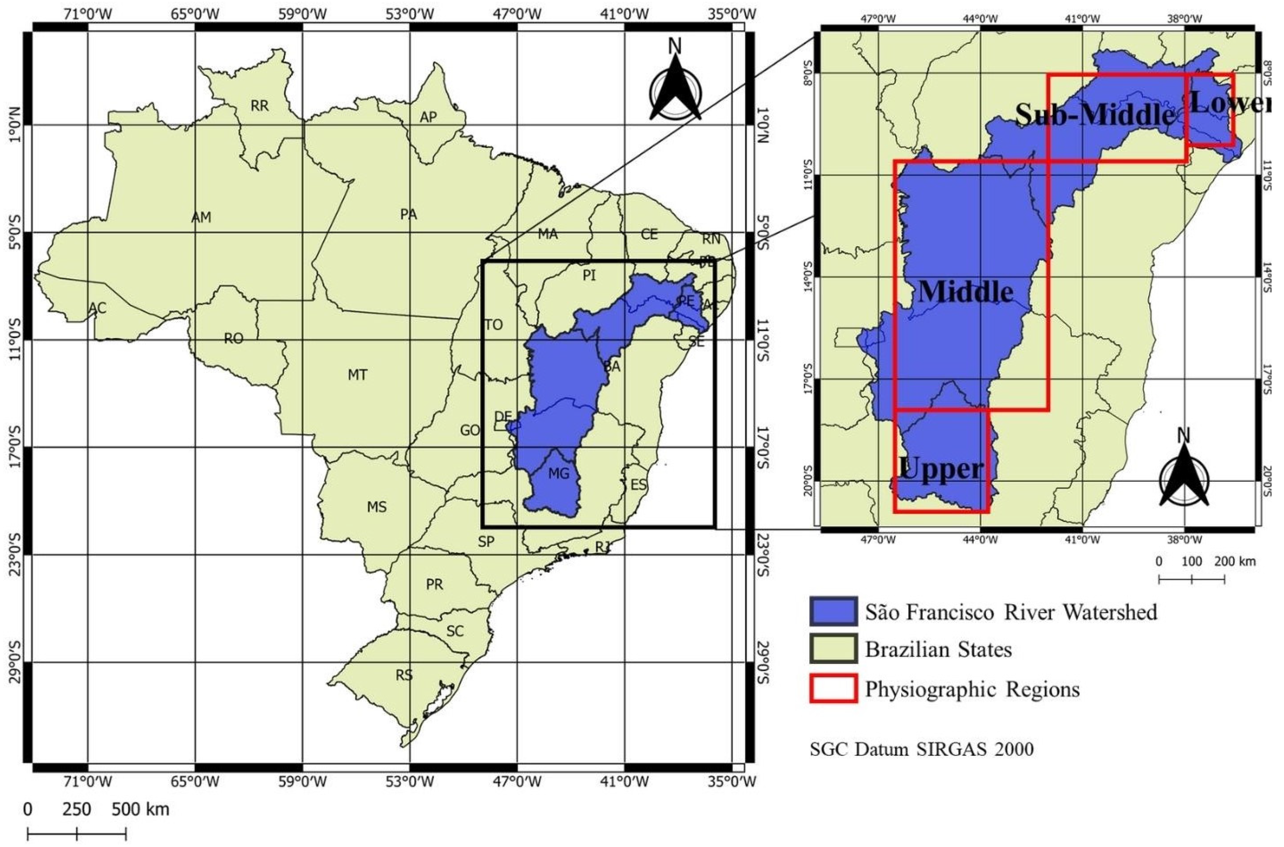
2.1. Study Area

The SFRB is one of the main Brazilian watersheds. This basin runs for 2863 km; crosses six Brazilian states [20]; and it is subdivided into four regions: Upper, Middle, Sub-Middle, and Lower SF (Figure 1) [67]. The SFRB stands out (a) for its power generation potential with important hydro power plants such as Três Marias, Sobradinho, Paulo Afonso, Itaparica, and Xingó and (b) for the water supply for the population and its activities, among other ecosystem services such as: navigability, fishing activities, agriculture, and basic sanitation [68].
The SFRB (Figure 1, left) covers an area of approximately 638,466 km2, comprises about 7.5% of the entire Brazilian territory, and has a population of over 14 million inhabitants [18,69]. Most of the population (7,075,587 people) is located in the Upper SF [69]. Along its physiographic regions, fragments of different biomes are found, such as: Cerrado in the Upper and Middle SF; Caatinga in the Middle, Sub-Middle, and Lower SF region; and the Atlantic Forest in the Upper region and in the coastal areas of the Lower SF [19,70].
Due to its territorial extension, different climate patterns are found in its subregions. According to the Köppen climate classification, the Upper SF has a predominance of Aw climate (warm and humid tropical, with dry winters); in the Middle SF, Aw and BShw (semiarid) prevail; the BShw climate predominates in the Sub-Middle region; and the As climate (warm and humid tropical, with rainy winters) in the Lower SF [71]. The precipitation patterns in the basin show a decrease from the headwater, which is located in the SEB (Upper SF) towards the mouth of the river located on the coast of the NEB (Lower SF) [72]. The main systems responsible for the precipitation in the SFRB are the SACZ [73,74,75] in the Upper and Middle SF and the ITCZ [76] in the Sub-Middle and Lower SF.

2.2. Data

Different datasets were used in the study. Precipitation data between 1979 and 2020 from the Gauge-Based Analysis of Global Daily Precipitation (CPC) generated by the National Oceanic and Atmospheric Administration/Climate Prediction Center (NOAA/CPC) were used. CPC has a spatial resolution of 0.5° and is constructed based on surface observations of approximately 30,000 stations distributed across the globe, which are interpolated to create a higher-quality unified set [77,78]. Therefore, the direct comparison of CPC interpolated data and rain gauge stations shows similar results [79]. For each SF sub-basin, Upper SF (20°75′ S/17°75′ S–46°50′ W/43°75′ W), Middle SF (17°75′ S/10°50′ S–46°50′ W/42°00′ W), Sub-Middle SF (10°50′ S/8°00′ S–42°00′ W/38°00′ W), and Lower SF (10°00′ S/8°00′ S–38°00′ W/36°75′ W; red boxes indicated in Figure 1 right), a monthly precipitation time series based on the areal average was constructed.
ERA5 Reanalysis [80] data for geopotential heights and zonal and meridional components of the wind at 850- and 250-hPa levels, sea surface temperature (SST), and mean sea level pressure (MSLP) were also analyzed. The data are provided by the European Center for Medium-Range Weather Forecasts (ECMWF) and have a spatial resolution of 0.25° (https://climate.copernicus.eu/climate-reanalysis, accessed on 30 April 2021). The 850- and 250-hPa levels were selected, as they best represent the South American low and high levels atmospheric circulation patterns, respectively [81]. At the 850-hPa level, the low-level jets of South America are represented without the influence of topography, while, at the 250-hPa level are the high-level jets and the Bolivian High-Pressure System [82].
The Tropical Southern Atlantic Index (TSA) [83] and the Oceanic Niño Index (ONI), both available on the National Oceanic and Atmospheric Administration (NOAA—https://psl.noaa.gov/data/climateindices/list/#Nina34, accessed on 11 August 2021), were used to indicate the anomalous conditions of the sea surface temperature in the Tropical South Atlantic and Central-East Pacific Oceans. The South Atlantic Subtropical Anticyclone Index (Índice do Anticiclone Subtropical do Atlântico Sul—IASAS) [84] was also included to control the MSLP over the SEB and Southern Brazil as a response of the South Atlantic Subtropical Anticyclone (SASA) influence. This index is obtained through the difference of MSLP over the SEB and Southern Brazil [84] and is available on the website of the Universidade Federal de Itajubá (UNIFEI—https://meteorologia.unifei.edu.br/teleconexoes/, accessed on 11 August 2021). When the IASAS is positive (negative), the MSLP is higher (lower) over the SEB and lower (higher) over the southern region. Then, the positive index phase indicates that the rainfall is concentrated over Southern Brazil, since the low-level jet east of the Andes flows in the direction of the lower pressure, contributing to the moisture convergence.

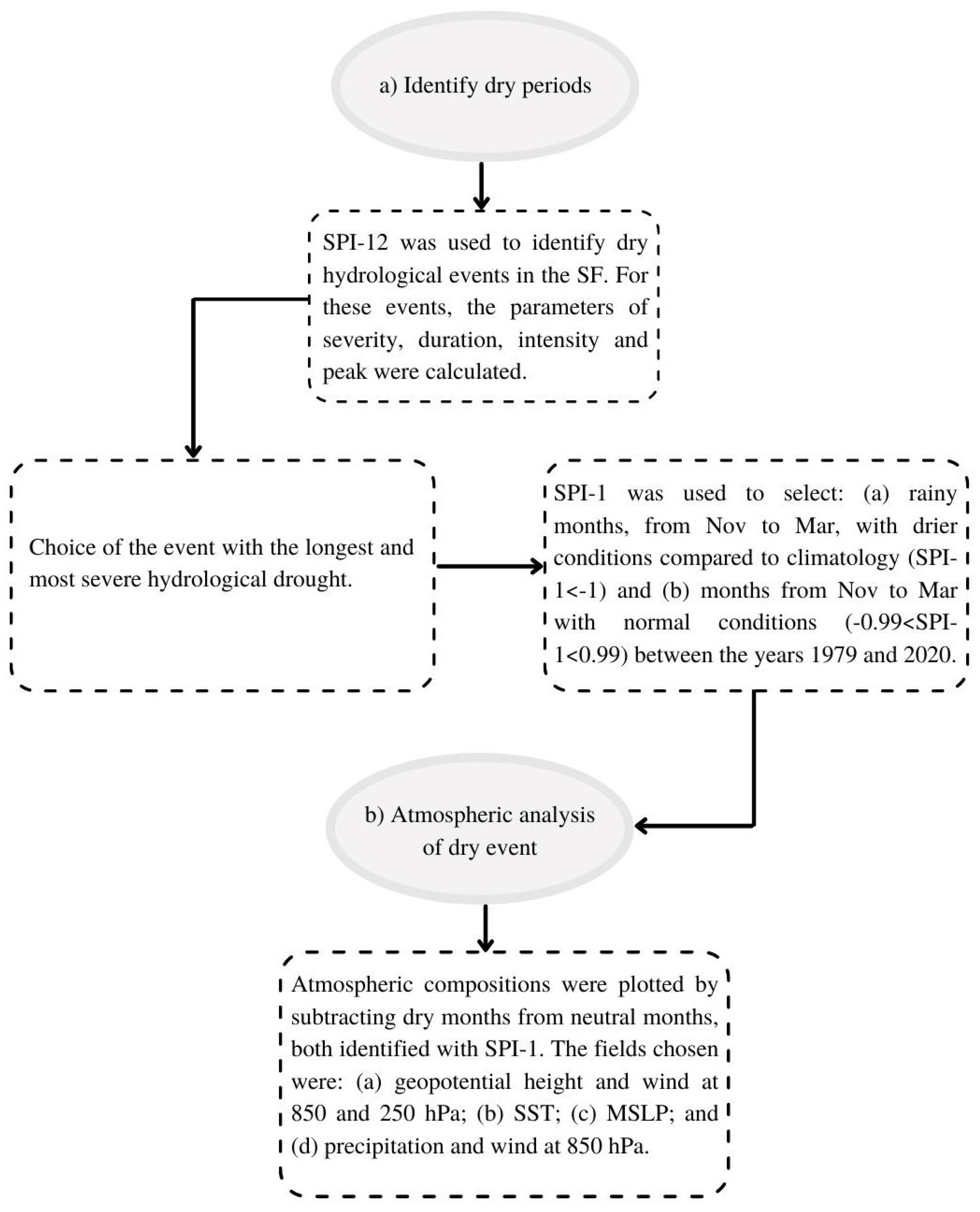
2.3. Identification of Dry Periods

The SPI is an index developed by McKee et al. [17] that uses only precipitation data to identify wet and dry periods. This index measures the precipitation anomalies in a given location by comparisons with the total rainfall accumulated rates for the reference period. The index can be calculated for different time scales of accumulation. The 1-month scale (SPI-1) can reflect short-term conditions and can be used for the analysis of meteorological droughts [1]. The 12-month scale (SPI-12), in addition to long-term precipitation patterns, can also be associated with anomalies of river flows and reservoir levels [1], and it was chosen to assess hydrological droughts in the SF, following Santos et al. [85]. By calculating the SPI, the time series is adjusted to a gamma function, and, after this process, it is transformed into a variable with normal distribution; therefore, the average of the SPI is always zero, and its variance has a unit value [86]. For its calculation, it is recommended to have no missing data, as described by Silva et al. [7], McKee et al. [17] and Guttman [87]. SPI-1 and SPI-12 were applied to identify the dry periods in the SF subregions between 1979 and 2020. The monthly rainfall series used in the SPI (SPI-1 and SPI-12) calculations had no missing data.
SPI positive values indicate rainy periods, while negative values characterize rainfall deficits. The onset of a drought episode can be identified when the SPI changes from a positive to a negative value, and it ends when the index returns to a positive value; however, to define the event as dry, the SPI must reach a value less than or equal to −1 [17]. Works such as Gozzo et al. [52], Stojanovic et al. [88] and Drumond et al. [89] also applied a similar methodology to assess the onset of events in order to include the mild dry conditions that lead to the establishment of a drought in the analysis. In addition to the criteria to define a drought, McKee et al. [17] created a system to classify the SPI values, as shown in Table 1. Hence, after the identification of SPI-12 drought episodes, the parameters of severity (absolute sum of all SPI-12 values during the event), duration (number of months between the first and last month of the event), intensity (ratio between severity and duration), and peak (highest absolute SPI-12 value registered during the event) were calculated according to McKee et al. [17].
For this analysis, the longest and most severe hydrological drought was identified through SPI-12. Afterwards, SPI-1 was used to select months during the rainy season that prevailed over the SFRB (from November to March), presenting anomalous dry conditions (SPI-1 is less than −1) within this event. In addition, SPI-1 was also applied to identify months with near-normal conditions (SPI-1 between −0.99 and 0.99) from November to March (Nov–Mar) during the period 1979–2020 (Figure 2).

2.4. Anomalous Atmospheric and Oceanic Patterns

Monthly composite maps were plotted using ERA5 to investigate the atmospheric and oceanic patterns associated with the meteorological dry conditions (identified via SPI-1) observed during the rainy season of the longest and most severe hydrological drought in the SFRB (identified by the SPI-12 analysis). The composite maps were computed by subtracting the average of the drier months identified through SPI-1 within the hydrological drought episode selected from the average of the near-normal months within the studied period (1979–2020). Both months (dry and normal) were identified with SPI-1.
Figure 2 summarizes the methodology applied in this work through a flow chart.

3. Results and Discussion

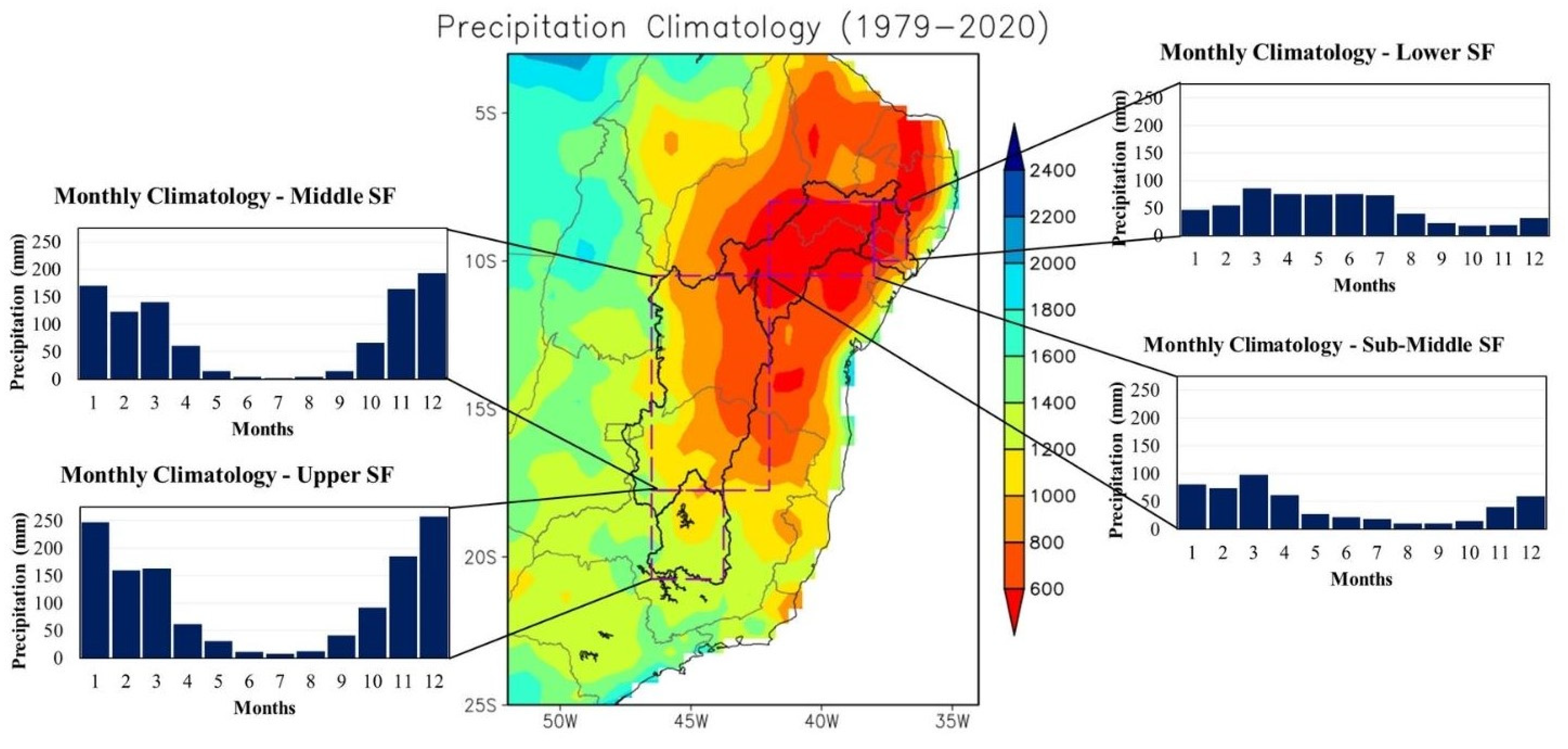
3.1. Climatology of Precipitation in the SFRB

The annual and monthly rainfall climatology in the SFRB, considering the period from 1979 to 2020, were calculated in order to identify the wet season in the subregions. The results are shown in Figure 3.
The rainfall regime in the basin presents temporal and spatial variability, agreeing with the results of Cruz et al. [90]. The highest annual accumulated rainfall is concentrated in the Upper and Middle SF regions, with 1200–1400 mm per year. In the Upper and Middle SF, the wettest months are November, December, January, February, and March, while the precipitation is the minimum during June, July, and August.
The total annual precipitation rates for the Sub-Middle and Lower SF are smaller, with values between 600 and 1000 mm per year. Differing from the other regions, the rainy season in the Lower SF is concentrated between the months of March, April, May, June, and July. In turn, the dry season occurs during the months of September, October, and November.
The rainfall annual cycle in the Upper and Middle SF regions follows the South American Monsoon precipitation regime, with wet summers and dry winters [82]. On the other hand, the precipitation cycle in the Sub-Middle and Lower SF is slightly different, mainly in the Lower SF, which is strongly influenced by the ITCZ that migrates to its southernmost position in the austral autumn months—wet season [82].

3.2. Identification of the Dry Periods

SPI-12 was used to assess the hydrological drought episodes between 1979 and 2020 in the four subregions (Table 2). Analyzing the parameters of severity and duration, the drought that affected the Upper SF in the last decade (2012–2020) was the most severe and the longest (in total, it lasted 103 months) among all the episodes identified in the four subregions. In addition, this episode peaked at 3.08 in January 2015 (Table 2), which refers to precipitation deficit conditions accumulated from February 2014 to January 2015 falling into the extreme drought category (as presented in Table 1). The major impacts of this extremely dry year were described in the literature and discussed in Section 1. Although not the objective of the present work, it would be interesting in further studies to investigate the anomalous climate patterns during the year that preceded this peak of −3.08 as an attempt to understand the extreme climate conditions involved.
Since the 2012–2020 drought in the Upper SF was the most severe and the longest among all the episodes identified for all subregions, this was the episode chosen for the analysis of the atmospheric and oceanic patterns. It is important to highlight that the period 2012–2020 also encompasses the SPI-12 drought episodes configured in the other subregions of the SFRB, indicating the predominance of dry conditions at the basin scale during these years. For instance, the Upper SF and Middle SF had very similar drought event distributions, with the Middle SF presenting only three months of accumulated humid conditions. The Sub-Middle SF was also affected by the SPI-12 drought during 2012–2018, presenting only three months of accumulated wet conditions. The period of 2012–2020 was also predominantly dry in the Lower SF.
Moreover, the largest part of the basin’s population lives in this subregion [69], and 70% of the flow of the entire SF river comes from this region and from part of the Middle SF [21]. Therefore, the lack of rainfall in the region can compromise the amount of water available along the basin. The results obtained through the SPI-12 analysis are in accordance with the ones obtained via different methodologies for the NEB [14,15,22,23]. Droughts were also detected in the SEB during the middle 2010s [25,26,53,54].
The months during the wet season (Nov–Mar) presenting: (a) dry conditions during the selected drought event (2012–2020) and (b) near-normal conditions within the entire period 1979–2020 were identified through the Upper SF SPI-1 time series, and the results are shown in Table 3. Within the drought event studied, the year 2014 was the only one with extremely dry conditions during three out of four months of the wet season (Dec–Feb), indicating the exceptionality of this year as pointed out by the SPI-12 peak in January 2015. Considering the entire study period, December was the month with the highest number of years with extreme drought conditions. In March, dry conditions were identified only twice, and both of them reached the category moderate. November was the only month of the rainy season that did not present dry conditions in any year of the selected event. Further details of the SPI-1 and SPI-12 time series are found in Figures S1 and S2 of the Supplementary Material.
Table 4 shows that the months with meteorological dry conditions in the Upper SF during the 2012–2020 event (Table 3) also encompassed the dry months identified for the other subregions, mainly during the months of Dec–Feb (austral summer). Following the same criteria applied in Table 3 for the Upper SF, the months of dry conditions between Nov and Mar for each subregion have been identified through their respective SPI-1 time series and are presented in Table 4, in which is considered the different drought events of each region within the period 2012–2020 (Table 2). This result justifies the representativeness of the results based on the 2012–2020 Upper SF analysis as the basin domain, in addition to its socioeconomic and hydrological issues already discussed. Even though the Lower SF has a distinct rainfall regime, the dry months of the austral summer coincide with the dry months of the Upper SF. The similarity in the dry periods is even higher between the Middle SF and Upper SF, which have a similar rainy season. Major differences were found during March, a rainy–dry transition month. While it is the dismissal of the rainy season in the Upper SF and Mid SF, the peak of precipitation in the Sub-Middle and the Lower SF normally occurs in March.

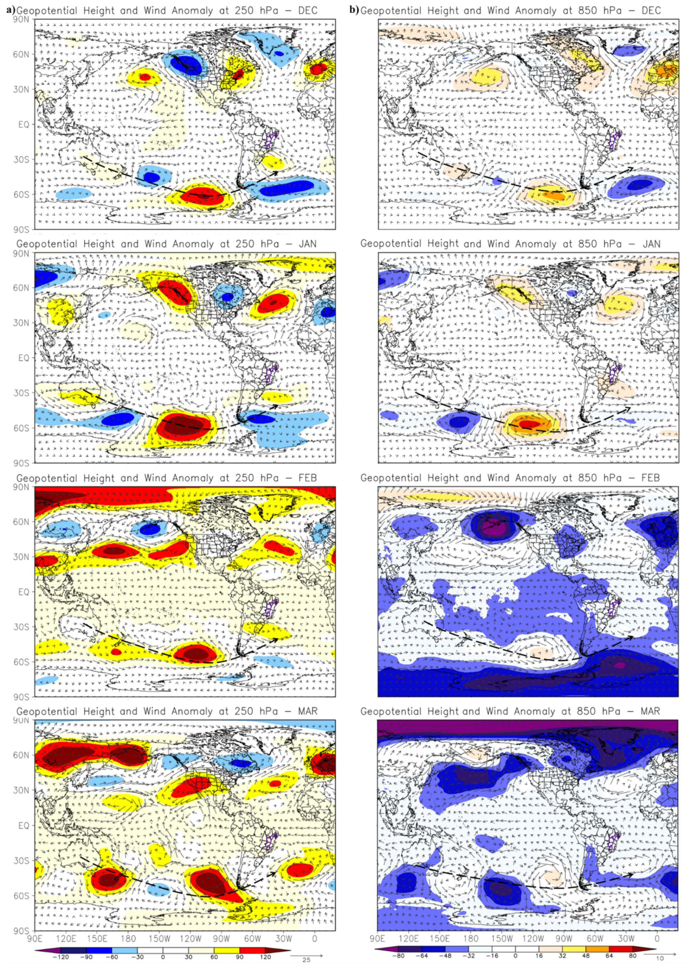
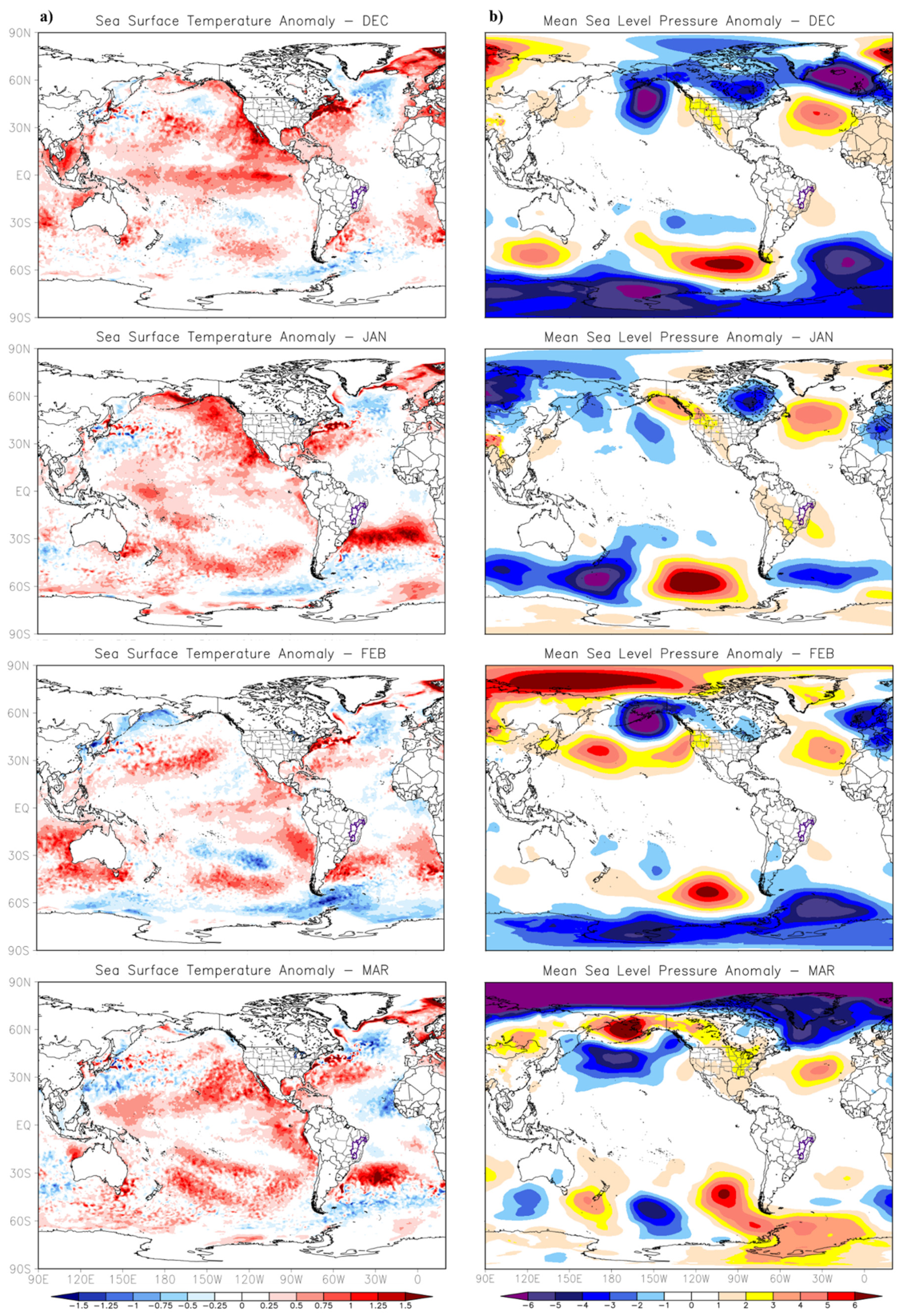
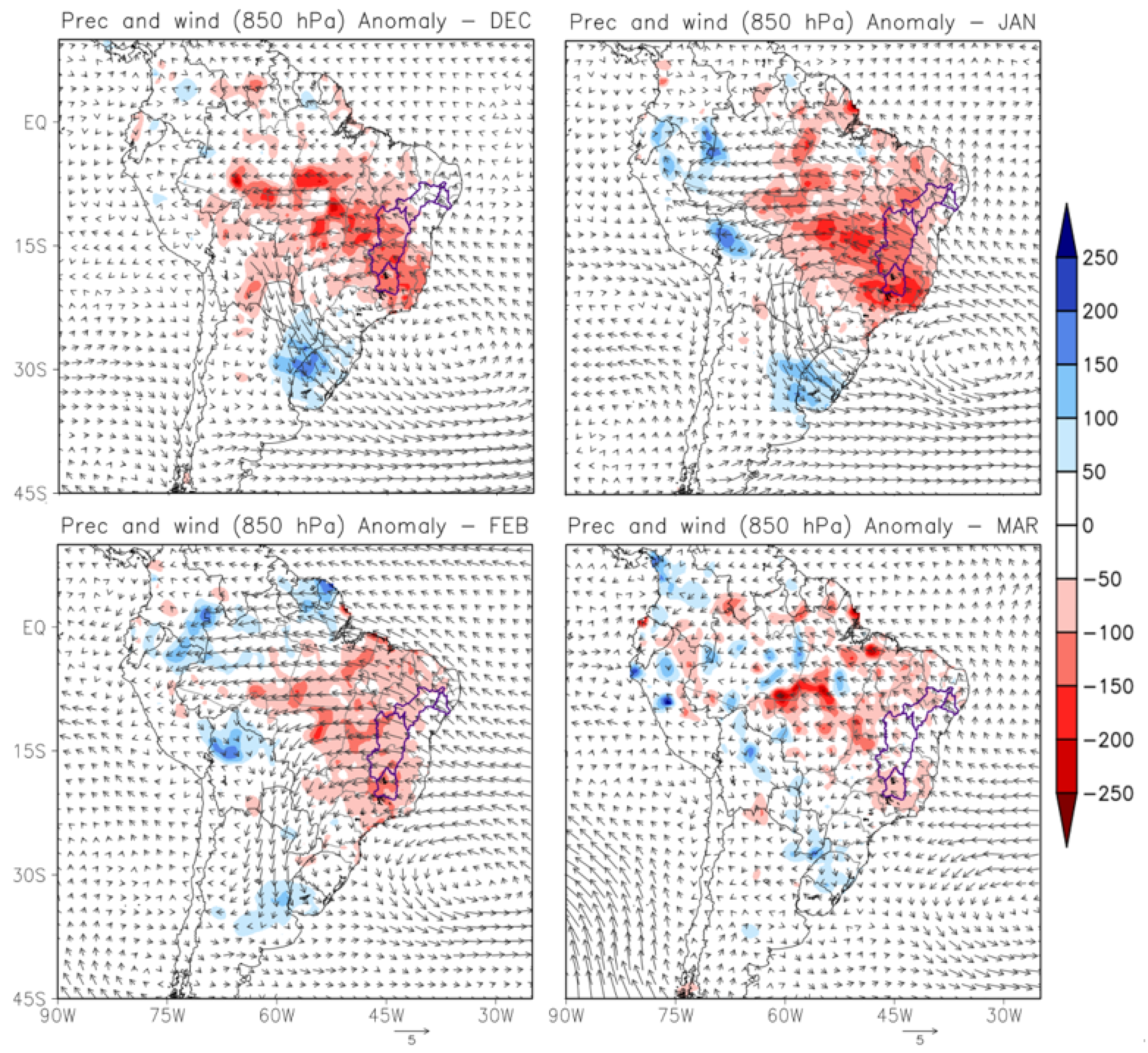
3.3. Anomalous Atmospheric and Oceanic Patterns

After the identification of the dry and normal months through SPI-1 for the Upper SF (shown in the Table 3), atmospheric field composite maps were made in order to verify the anomalous atmospheric and oceanic patterns associated with dry conditions. These composite maps were plotted by subtracting the average of variables in the dry months, within the hydrological drought event, from the average of the variables in the normal months for the entire period. As the month of November did not present any year with a dry condition within the analyzed event, the composite maps were made considering only the dry months from December to March.
The geopotential height composite map and wind at 850 and 250 hPa shows a wave propagation pattern from the vicinity of Australia through Southern South America to the SEB region of Brazil (Figure 4a,b) through all months (Dec–Mar). In the SEB, this pattern reaches positive values of geopotential height and anticyclonic atmospheric circulation, which characterizes a region with a high atmospheric pressure system. This circulation pattern, shown in Figure 4, is similar to the anomalous patterns found for the drought associated with the Brazilian energy crisis in 2001 [91] and the water crisis in the SEB in 2014 [54].
The Tropical Atlantic Ocean shows conditions closer to the climatological features, while the Tropical Pacific Ocean does not indicate El Niño and La Niña conditions, which can be confirmed by the indices shown in Table 4. In the South Atlantic Ocean, patterns similar to those shown in Figure 4 are also found through the MSLP composite map (Figure 5b). Between 30° S and 60° S latitudes, there is a predominance of positive SST anomalies (Figure 5a) and a high atmospheric pressure system. In the presence of high-pressure anomalies, solar energy can more efficiently warm the ocean surface. Therefore, there is a combination of processes: an anomalous wave propagation pattern favors the predominance of anticyclonic anomalies close to the Brazilian coast, which, in turn, hinder the formation of precipitation systems, so that the sky becomes less cloudy and there is a more effective warming of the SST [53,54].
The composite map of precipitation anomaly for each month from Dec to Mar within the period 2012–2020 shows a deficit of precipitation in several regions of the country (Figure 6). The SEB and NEB regions were the most affected, with rainfall deficits reaching 250 mm in Jan. The SEB faced a serious water crisis between 2014 and 2016, as studied by Coelho et al. [25], Finke et al. [26] and Marengo et al. [53]. Regarding the low-level wind anomaly, there was an anomalous anticyclonic circulation on or near the south and SEB coast. In March, when this system was further away from the coast, the dry conditions were milder. Confirming the result already found through the SPI-12 analysis, the precipitation anomaly composite map shows the Upper SF region as the most affected by the deficit of precipitation. The largest negative rainfall anomalies are associated with the presence of a positive MSLP anomaly near the coast of SEB Brazil (Figure 5b). This anomalous high pressure seemed to enhance the flow of the low-level jet east of the Andes towards Southeastern South America (Figure 6), then favored shaping a precipitation dipole between the south and SEB. In this dipole, the lack of rain in the region of the SACZ is associated with above-average precipitation in the southern region of the country or vice-versa [41,45,92,93]. These anomalous precipitation and low-level circulation patterns were also similar to the ones registered in the energy crisis in 2001 [91].
In general, the anomalous atmospheric patterns shown in this study were similar to those that occurred in the water crisis in the SEB in 2014 [54], indicating that the dry conditions observed during the 2012–2020 episode over the Upper-SF investigated here have also affected other regions in the country [89,94]. The predominance of the wave pattern with positive pressure anomaly over the SEB may inhibit cloud formation, which can consequently warm the SST, as noted by the positive anomalies of the SST in the South Atlantic (Figure 5a). The presence of the positive pressure anomaly over the SEB inhibits the transport of moisture from the interior of the continent to the SEB region. On the other hand, the southern region tends to show positive precipitation anomalies.
The higher values of atmospheric pressure in the SEB can also be identified by the IASAS index, which is a measure of the difference in the MSLP between the SEB and south regions of Brazil. Therefore, between Dec and Mar from 2012 to 2020, there was a positive IASAS, indicating higher MSLP over the SEB region. The Pearson correlation coefficient was calculated between the IASAS, TSA, and ONI indices with the SPI-1 time series to verify the linear relationship between the SASA, the Southern Tropical Atlantic, and ENSO with the monthly precipitation variability in Upper SF during 1979–2020. To test the significance of this result, the bilateral t-test was applied considering 40 degrees of freedom (subtracting 2 years from the 42 years of the study period) at a significance level of 0.01. The negative correlation between the IASAS and Upper-SF SPI-1 (Table 5) also supports these results from a climatological perspective. Hence, dry conditions in the Upper SF during the summer months are associated with a positive MSLP anomaly in the SEB and negative in Southern Brazil. It was not the focus of this study, but for further studies, the dynamics of rainfall distribution in the other subregions may be analyzed through the correlation of the SPI-1 time series with the indices, considering the different rainy periods.

4. Conclusions

The drivers of droughts in the SFRB region are discussed little, although there are several studies that have identified periods of drought in the basin region. Thus, the present study used the SPI to identify the hydrological drought periods in the SFRB and, for the longest and most severe hydrological drought, analyzed the atmospheric and oceanic patterns that were associated with dry conditions in the rainy season. The SPI-12 analysis showed that all subregions of the SFRB experienced long and extreme hydrological drought episodes in the 2010s. According to the methodology applied, the Upper SF region stands out with the longest (103 months; 2012–2020) and the most severe drought when compared with all the droughts identified for the four subregions between 1979 and 2020.
The analysis of the atmospheric and oceanic composite maps anomalies, obtained through the differences between the anomalous dry and normal conditions months (identified by SPI-1 of the Upper SF) during the rainy season, showed that the rainfall deficit, which affected several regions of the country between 2012 and 2020, was associated with an anomalous wave propagation pattern of Australia origin. This pattern favored the predominance of an anticyclonic system near the coast of the SEB, which probably acted by inhibiting the formation of rain clouds, resulting in an increase in the SST in the region. This condition leads to a decrease of the precipitation rates in the SEB region and causes a positive rainfall anomaly in the south region of the country. The IASAS index, which controls the SASA, presents positive values in almost all the anomalous dry months considered in the composite maps analysis, agreeing with the pressure anomaly composite maps. Climatologically, the negative linear correlation between the IASAS and Upper SF SPI-1 time series indicates that the occurrence of an anomalous high atmospheric pressure system near the SEB coast of Brazil inhibits precipitation in the Upper SF region. Although not the scope of this study, further investigation of the potential forcing that triggers the wave propagated in the vicinity of Australia is necessary, as well as a more in-depth study on the IASAS and the Southern Atlantic variability. Previous studies showed the importance of the South Atlantic Ocean as a moisture source for Eastern South America [89,94,95,96].

Supplementary Materials

The following are available online at https://www.mdpi.com/article/10.3390/atmos13010041/s1: Figure S1: SPI-1 time series for the four SF regions for the period Jan 1979–Dec 2020. Figure S2: SPI-12 time series for the four SF regions for the period Jan 1980–Dec 2020.

Author Contributions

Conceptualization, A.A.F., A.D., V.S.B.C. and M.S.R.; methodology, A.A.F.; analysis, A.A.F., A.D., V.S.B.C. and M.S.R.; writing—original draft preparation, A.A.F., A.D., V.S.B.C. and M.S.R.; and writing—review and editing, A.A.F., A.D., V.S.B.C., M.S.R., B.C.S. and C.B.U. All authors have read and agreed to the published version of the manuscript.

Funding

This work is part of the project GlobalHydroPressure (EU Water JPI). A.A.F. and V.S.B.C. acknowledge the support received by the Minas Gerais Research Funding Foundation—FAPEMIG (ID-11831). V.S.B.C., M.S.R. and B.C.S. also acknowledge FAPEMIG (APQ 04377-18). A.D. acknowledges the support from the Brazilian National Council for Scientific and Technological Development (CNPq) (100186/2021-1). C.B.U. acknowledge the support received from the Swedish Research Council FORMAS, Grant No. 2018-02379).

Data Availability Statement

All dataset used in this study are available by meteorological centers.

Acknowledgments

The authors would like to thank the Coordination for the Improvement of Higher Education Personnel (CAPES), the Minas Gerais Research Funding Foundation (FAPEMIG), and the Brazilian National Council for Scientific and Technological Development (CNPq). We would like to thank ECMWF and CPC for providing the data. The authors would like to thank the editor and the anonymous reviewers.

Conflicts of Interest

The authors declare no conflict of interest. The funders had no role in the design of the study; in the collection, analyses, or interpretation of the data; in the writing of the manuscript; or in the decision to publish the results.

References

  1. WMO—World Meteorological Organization. Standardized Precipitation Index. User Guide. 2012. Available online: https://library.wmo.int/doc_num.php?explnum_id=7768 (accessed on 17 November 2020).
  2. Van Loon, A.F.; Gleeson, T.; Clark, J.; Van Dijk, A.I.J.M.; Stahl, K.; Hannaford, J.; Baldasarre, G.; Teuling, A.J.; Tallaksen, L.M.; Uijlenhoet, R.; et al. Drought in the Anthropocene. Nat. Geosci. 2016, 9, 89–91. [Google Scholar] [CrossRef] [Green Version]
  3. Wilhite, D.A.; Glantz, M.H. Understanding: The drought phenomenon: The role of definitions. Water Int. 1985, 10, 111–120. [Google Scholar] [CrossRef] [Green Version]
  4. Yihdego, Y.; Vaheddoost, B.; Al-Weshah, R.A. Drought indices and indicators revisited. Arab. J. Geosci. 2019, 12, 69. [Google Scholar] [CrossRef]
  5. WMO—World Meteorological Organization; GWP—Global Water Partnership. Handbook of Drought Indicators and Indices; World Meteorological Organization: Geneva, Switzerland, 2016; Available online: https://public.wmo.int/en/resources/library/handbook-of-drought-indicators-and-indices (accessed on 5 November 2021).
  6. Mukherjee, S.; Mishra, A.; Trenberth, K.E. Climate change and drought: A perspective on drought indices. Curr. Clim. Chang. Rep. 2018, 4, 145–163. [Google Scholar] [CrossRef]
  7. Da Silva, D.F.; da Silva Lima, M.J.; de Souza Neto, P.F.; Gomes, H.B.; dos Santos Silva, F.D.; de Carvalho Almeida, H.R.R.; Pereira, M.P.S.; Costa, R.L. Caracterização de eventos extremos e de suas causas climáticas com base no índice Padronizado de Precipitação Para o Leste do Nordeste. RBGF 2020, 13, 449–464. [Google Scholar] [CrossRef]
  8. Rossato, L.; Marengo, J.A.; de Angelis, C.F.; Pires, L.B.M.; Mendiondo, E.M. Impact of soil moisture over Palmer Drought Severity Index and its future projections in Brazil. RBRH 2017, 22, e36. [Google Scholar] [CrossRef] [Green Version]
  9. Gozzo, L.F.; Palma, D.S.; Custodio, M.S.; Machado, J.P. Climatology and trend of severe drought events in the state of São Paulo, Brazil, during the 20th century. Atmosphere 2019, 10, 190. [Google Scholar] [CrossRef] [Green Version]
  10. Gonçalves, S.T.N.; das Chagas Vasconcelos Junior, F.; Sakamoto, M.S.; da Silva Silveira, C.; Martins, E.S.P.R. Índices e Metodologias de Monitoramento de Secas: Uma Revisão. Rev. Bras. Meteorol. 2021, 36, 495–511. [Google Scholar] [CrossRef]
  11. Morello, T.F.; Ramos, R.M.; Anderson, L.O.; Owen, N.; Rosan, T.M.; Steil, L. Predicting fires for policy making: Improving accuracy of fire brigade allocation in the Brazilian Amazon. Ecol. Econ. 2020, 169, 106501. [Google Scholar] [CrossRef]
  12. Martins, M.A.; Tomasella, J.; Rodriguez, D.A.; Alvalá, R.C.S.; Giarolla, A.; Garofolo, L.L.; Siqueira Júnior, J.L.; Paolicchi, L.T.L.C.; Pinto, G.L.N. Improving drought management in the Brazilian semiarid through crop forecasting. Agric. Syst. 2018, 160, 21–30. [Google Scholar] [CrossRef]
  13. Silva, S.M.; Souza Filho, F.A.; Araújo, L.M., Jr. Mecanismo financeiro projetado com índices de seca como instrumento de gestão de risco em recursos hídricos. Rev. Bras. Recur Hídricos 2015, 20, 320–330. [Google Scholar] [CrossRef]
  14. Cunha, A.P.M.A.; Zeri, M.; Leal, K.D.; Costa, L.; Cuartas, L.A.; Marengo, J.A.; Tomasella, J.; Vieira, R.M.; Barbosa, A.A.; Cunningham, C.; et al. Extreme drought events over Brazil from 2011 to 2019. Atmosphere 2019, 10, 642. [Google Scholar] [CrossRef] [Green Version]
  15. Brito, S.S.B.; Cunha, A.P.M.; Cunningham, C.C.; Alvalá, R.C.; Marengo, J.A.; Carvalho, M.A. Frequency, duration and severity of drought in the Semiarid Northeast Brazil region. Int. J. Climatol. 2017, 38, 517–529. [Google Scholar] [CrossRef]
  16. Xavier, L.C.P.; Silva, S.M.O.D.; Carvalho, T.M.N.; Pontes Filho, J.D.; Souza Filho, F.D.A.D. Use of Machine Learning in Evaluation of Drought Perception in Irrigated Agriculture: The Case of an Irrigated Perimeter in Brazil. Water 2020, 12, 1546. [Google Scholar] [CrossRef]
  17. Mckee, T.B.; Doesken, N.J.; Kleist, J. The Relationship of Drought Frequency and Duration to Time Scales. In Proceedings of the 8th Conference on Applied Climatology, Boston, MA, USA, 17–22 January 1993; pp. 179–183. Available online: https://climate.colostate.edu/pdfs/relationshipofdroughtfrequency.pdf (accessed on 10 November 2020).
  18. ANA—Agência Nacional De Águas E Saneamento Básico. Conjuntura dos Recursos Hídricos no Brasil: Regiões Hidrográficas Brasileiras—Edição Especial; ANA: Brasília, Brazil, 2015. Available online: https://www.snirh.gov.br/portal/centrais-de-conteudos/conjuntura-dos-recursos-hidricos/regioeshidrograficas2014.pdf (accessed on 3 August 2020).
  19. CODEVASF—Companhia de Desenvolvimento dos Vales do São Francisco e do Parnaíba. Plano Nascente: Plano de Preservação e Recuperação de Nascentes da Bacia do rio São Francisco; Editora IABS: Brasília Brasil, 2015; Available online: https://www.terrabrasilis.org.br/ecotecadigital/images/abook/pdf/2016/Marco/Mar.16.25.pdf (accessed on 15 March 2020).
  20. CBHSF—Comitê da Bacia do São Francisco. A Bacia. 2021. Available online: https://cbhsaofrancisco.org.br/a-bacia/ (accessed on 14 August 2021).
  21. Amorim, R.S.; De Souza, S.A.; Reis, D.S., Jr. Autocorrelation and Multiple Testing Procedures in Trend Detection Analysis: The Case Study of Hydrologic Extremes in São Francisco River Basin, Brazil. In Proceedings of the World Environmental and Water Resources Congress, Sacramento, CA, USA, 21–25 May 2017; pp. 134–148. Available online: https://ascelibrary.org/doi/abs/10.1061/9780784480601.013 (accessed on 22 October 2021).
  22. Marengo, J.A.; Cunha, A.P.; Alves, L.M. A Seca de 2012-15 no Semiárido do Nordeste do Brasil no Contexto Histórico. Climanálise 2016, 3, 1–6. Available online: http://climanalise.cptec.inpe.br/~rclimanl/revista/pdf/30anos/marengoetal.pdf (accessed on 22 June 2020).
  23. De Medeiros, F.J.; De Oliveira, C.P.; Silva, C.M.S.E.; De Araújo, J.M. Numerical simulation of the circulation and tropical teleconnection mechanisms of a severe drought event (2012–2016) in Northeastern Brazil. Clim. Dyn. 2020, 54, 4043–4057. [Google Scholar] [CrossRef]
  24. Paredes-Trejo, F.; Barbosa, H.A.; Giovannettone, J.; Kumar, T.V.; Thakur, M.K.; Buriti, C.D.O.; Uzcátegui-Briceño, C. Drought Assessment in the São Francisco River Basin Using Satellite-Based and Ground-Based Indices. Remote Sens. 2021, 13, 3921. [Google Scholar] [CrossRef]
  25. Coelho, C.A.S.; Cardoso, D.H.F.; Firpo, M.A. A seca de 2013 a 2015 na região sudeste do Brasil. Climanálise 2016, 30, 55–66. Available online: http://climanalise.cptec.inpe.br/~rclimanl/revista/pdf/30anos/Coelhoetal.pdf (accessed on 12 August 2021).
  26. Finke, K.; Jiménez-Esteve, B.; Taschetto, A.S.; Ummenhofer, C.C.; Bumke, K.; Domeisen, D.I.V. Revisiting remote drivers of the 2014 drought in South-Eastern Brazil. Clim. Dyn. 2020, 55, 3197–3211. [Google Scholar] [CrossRef]
  27. Geirinhas, J.L.; Russo, A.; Libonati, R.; Sousa, P.M.; Miralles, D.G.; Trigo, R.M. Recent increasing frequency of compound summer drought and heatwaves in Southeast Brazil. Environ. Res. Lett. 2021, 16, 034036. Available online: https://iopscience.iop.org/article/10.1088/1748-9326/abe0eb (accessed on 6 November 2021). [CrossRef]
  28. Munich, R.E. Natural Catastrophes 2014. Analyzes, Assessments, Positions. TOPICS-GEO 2014. 2015. Available online: https://www.munichre.com/content/dam/munichre/contentlounge/website-pieces/documents/302-08606_en.pdf/_jcr_content/renditions/original.media_file.download_attachment.file/302-08606_en.pdf (accessed on 8 November 2021).
  29. Reboita, M.S.; De Oliveira, D.D.; De Freitas, C.H.; De Oliveira, G.M.; Pereira, R.A.A. Anomalias dos Padrões Sinóticos da Atmosfera na América do Sul nos Meses de Janeiros de 2014 e 2015. Rev. Bras. Energ. Renov. 2015, 4, 1–12. [Google Scholar] [CrossRef] [Green Version]
  30. Nobre, C.A.; Marengo, J.A.; Seluchi, M.E.; Cuartas, L.A.; Alves, L.M. Some characteristics and impacts of the drought and water crisis in Southeastern Brazil during 2014 and 2015. J. Water Resour. Prot. 2016, 8, 252–262. [Google Scholar] [CrossRef] [Green Version]
  31. Gutiérrez, A.P.A.; Engle, N.L.; De Nys, E.; Molejón, C.; Martins, E.S. Drought preparedness in Brazil. Weather Clim. Extrem. 2014, 3, 95–106. [Google Scholar] [CrossRef] [Green Version]
  32. Marengo, J.A.; Torres, R.R.; Alves, L.M. Drought in Northeast Brazil—Past, present, and future. Theor. Appl. Climatol. 2016, 129, 1189–1200. [Google Scholar] [CrossRef]
  33. Marengo, J.A.; Alves, L.M.; Beserra, E.A.; Lacerda, F.F. Variabilidade e Mudanças Climáticas no Semiárido Brasileiro. Recursos Hídricos em Regiões Áridas e Semiáridas. 2011. Volume 1. Available online: http://plutao.sid.inpe.br/col/dpi.inpe.br/plutao/2011/06.11.02.16/doc/Marengo_Variabilidade.pdf?languagebutton=en (accessed on 14 August 2020).
  34. SUDENE—Superintendência do Desenvolvimento do Nordeste. Nova Delimitação Semiárido. 2018. Available online: http://antigo.sudene.gov.br/images/arquivos/semiarido/arquivos/Rela%C3%A7%C3%A3o_de_Munic%C3%ADpios_Semi%C3%A1rido.pdf (accessed on 14 August 2020).
  35. Santana, M.O. Atlas das Áreas Susceptíveis a Desertificação do Brasil/MMA; Secretaria de Recursos Hídricos: Brasília, Brazil, 2007; Available online: http://repiica.iica.int/docs/B3826p/B3826p.pdf (accessed on 9 October 2020).
  36. Perez-Marin, A.M.; Cavalcante, A.D.M.B.; Medeiros, S.S.D.; Tinôco, L.B.D.M.; Salcedo, I.H. Núcleos de Desertificação do Semiárido Brasileiro: Ocorrência Natural ou Antrópica? Parcer. Estratégicas 2013, 17, 87–106. Available online: http://seer.cgee.org.br/index.php/parcerias_estrategicas/article/viewFile/671/615 (accessed on 9 October 2020).
  37. Tomasella, J.; Vieira, R.M.S.P.; Barbosa, A.A.; Rodriguez, D.A.; Santana, M.O.; Sestini, M.F. Desertification trends in the Northeast of Brazil over the period 2000–2016. Int. J. Appl. Earth Obs. Geoinf. 2018, 73, 197–206. [Google Scholar] [CrossRef]
  38. Vieira, R.M.S.P.; Tomasella, J.; Barbosa, A.A.; Martins, M.A.; Rodriguez, D.A.; De Rezende, F.S.; Carriello, F.; Santana, M.O. Desertification risk assessment in Northeast Brazil: Current trends and future scenarios. Land Degrad. Dev. 2021, 32, 224–240. [Google Scholar] [CrossRef]
  39. MMA—Ministério do Meio Ambiente. Programa de Ação Nacional de Combate à Desertificação e Mitigação dos Efeitos da Seca; Secretaria de Recursos Hídricos: Brasilia, Brazil, 2005. Available online: https://antigo.mma.gov.br/estruturas/sedr_desertif/_arquivos/pan_brasil_portugues.pdf (accessed on 9 June 2021).
  40. De Almeida, C.; Barbieri, A.F.; Rodrigues Filho, S. Linking migration, climate and social protection in Brazilian semiarid: Case studies of Submédio São Francisco and Seridó Potiguar. SiD 2020, 11, 238–251. [Google Scholar] [CrossRef]
  41. Nogués-Paegle, J.; Mo, K.C. Alternating wet and dry conditions over South America during summer. Mon. Weather Rev. 1997, 125, 279–291. [Google Scholar] [CrossRef]
  42. Ambrizzi, T.; De Souza, E.B.; Pulwarty, R.S. The Hadley and Walker Regional Circulations and Associated ENSO Impacts on South American Seasonal Rainfall. In The Hadley Circulation: Present, Past and Future; Springer: Dordrecht, The Netherlands, 2005; pp. 203–235. [Google Scholar] [CrossRef]
  43. Tedeschi, R.G.; Grimm, A.M.; Cavalcanti, I.F.A. Influence of Central and East ENSO on extreme events of precipitation in South America during austral spring and summer. Int. J. Climatol. 2015, 35, 2045–2064. [Google Scholar] [CrossRef]
  44. Cai, W.; Mcphaden, M.J.; Grimm, A.M.; Rodrigues, R.R.; Taschetto, A.S.; Garreaud, R.D.; Dewitte, B.; Poveda, G.; Ham, Y.; Santoso, A.; et al. Climate impacts of the El Niño–southern oscillation on South America. Nat. Rev. Earth Environ. 2020, 1, 215–231. [Google Scholar] [CrossRef]
  45. Reboita, M.S.; Ambrizzi, T.; Crespo, N.M.; Dutra, L.M.M.; de S Ferreira, G.W.; Rehbein, A.; Drumond, A.; Da Rocha, R.P.; De Souza, C.A.D. Impacts of teleconnection patterns on South America climate. Ann. N. Y. Acad. Sci. 2021, 1504, 1–38. [Google Scholar] [CrossRef] [PubMed]
  46. Moura, A.D.; Shukla, J. On the dynamics of droughts in northeast Brazil: Observations, theory and numerical experiments with a general circulation model. J. Atmos. Sci. 1981, 38, 2653–2675. [Google Scholar] [CrossRef] [Green Version]
  47. Hastenrath, S.; Greischar, L. Circulation mechanisms related to northeast Brazil rainfall anomalies. J. Geophys. Res. Atmos. 1993, 98, 5093–5102. [Google Scholar] [CrossRef]
  48. Nobre, P.; Shukla, J. Variations of sea surface temperature, wind stress, and rainfall over the tropical Atlantic and South America. J. Clim. 1996, 9, 2464–2479. [Google Scholar] [CrossRef]
  49. Andreoli, R.V.; Kayano, M.T. Tropical Pacific and South Atlantic effects on rainfall variability over Northeast Brazil. Int. J. Climatol. J. R. Meteorol. Soc. 2006, 26, 1895–1912. [Google Scholar] [CrossRef]
  50. Hastenrath, S. Exploring the climate problems of Brazil’s Nordeste: A review. Clim. Chang. 2012, 112, 243–251. [Google Scholar] [CrossRef]
  51. Foltz, G.R.; Brandt, P.; Richter, I.; Rodríguez-Fonseca, B.; Hernandez, F.; Dengler, M.; Rodrigues, R.R.; Schmidt, J.O.; Yu, L.; Lefevre, N.; et al. The tropical Atlantic observing system. Front. Mar. Sci. 2019, 6, 206. [Google Scholar] [CrossRef]
  52. Gozzo, L.F.; Palma, D.S.; Custódio, M.S.; Drumond, A. Padrões Climatológicos Associados a Eventos de Seca no Leste do Estado de São Paulo. Rev. Bras. Climatol. 2021, 28, 321–341. [Google Scholar] [CrossRef]
  53. Marengo, J.A.; Nobre, C.A.; Seluchi, M.E.; Cuartas, A.; Alves, L.M.; Mendiondo, E.M.; Obregón, G.; Sampaio, G. A seca e a crise hídrica de 2014–2015 em São Paulo. Rev. USP 2015, 106, 31–44. [Google Scholar] [CrossRef] [Green Version]
  54. Coelho, C.A.S.; De Oliveira, C.P.; Ambrizzi, T.; Reboita, M.S.; Carpenedo, C.B.; Campos, J.L.P.S.; Tomaziello, A.C.N.; Pampuch, L.A.; Custódio, M.S.; Dutra, L.M.M.; et al. The 2014 southeast Brazil austral summer drought: Regional scale mechanisms and teleconnections. Clim. Dyn. 2015, 46, 3737–3752. [Google Scholar] [CrossRef]
  55. Marengo, J.A. Mudanças Climáticas e Eventos Extremos no Brasil; FBDS: Rio de Janeiro, Brazil, 2009; Available online: http://www.fbds.org.br/cop15/FBDS_MudancasClimaticas.pdf (accessed on 14 August 2020).
  56. PBMC—Painel Brasileiro de Mudanças Climáticas. Base Científica das Mudanças Climáticas. Contribuição do Grupo de Trabalho 1 do Painel Brasileiro de Mudanças Climáticas ao Primeiro Relatório da Avaliação Nacional Sobre Mudanças Climáticas; Ambrizzi, T., Araujo, M., Eds.; COPPE. Universidade Federal do Rio de Janeiro: Rio de Janeiro, Brasil, 2014; p. 464. Available online: http://www.pbmc.coppe.ufrj.br/documentos/RAN1_completo_vol1.pdf (accessed on 14 August 2020).
  57. Reboita, M.S.; Kuki, C.A.C.; Marrafon, V.H.; De Souza, C.A.; Ferreira, G.W.S.; Teodoro, T.; Lima, J.W.M. South America climate change revealed through climate indices projected by GCMs and Eta-RCM ensembles. Clim. Dyn. 2021, 1–27. [Google Scholar] [CrossRef]
  58. Marengo, J.A.; Chou, S.C.; Kay, G.; Alves, L.M.; Pesquero, J.F.; Soares, W.R.; Santos, D.C.; Lyra, A.A.; Sueiro, G.; Betts, R.; et al. Development of regional future climate change scenarios in South America using the Eta CPTEC/HadCM3 climate change projections: Climatology and regional analyses for the Amazon, São Francisco and the Paraná River basins. Clim. Dyn. 2012, 38, 1829–1848. [Google Scholar] [CrossRef]
  59. Marengo, J.A.; Cunha, A.P.; Soares, W.R.; Torres, R.R.; Alves, L.M.; Brito, S.S.B.; Cuartas, L.A.; Leal, K.; Ribeiro Neto, G.; Alvalá, R.C.S.; et al. Increase risk of drought in the semiarid lands of Northeast Brazil due to regional warming above 4 °C. In Climate Change Risks in Brazil; Springer: Cham, Switzerland, 2019; pp. 181–200. [Google Scholar] [CrossRef]
  60. Marengo, J.A. O futuro clima do Brasil. Rev. USP 2014, 103, 25–32. [Google Scholar] [CrossRef] [Green Version]
  61. Lyra, A.; Tavares, P.; Chou, S.C.; Sueiro, G.; Dereczynski, C.; Sondermann, M.; Silva, A.; Marengo, J.; Giarolla, A. Climate change projections over three metropolitan regions in Southeast Brazil using the non-hydrostatic Eta regional climate model at 5-km resolution. Theor. Appl. Climatol. 2017, 132, 663–682. [Google Scholar] [CrossRef]
  62. Reboita, M.S.; Marrafon, V.H.A.; Llopart, M.; Da Rocha, R.P. Cenários de mudanças climáticas projetados para o estado de Minas Gerais. Rev. Bras. Climatol. 2018, 1, 110–128. [Google Scholar] [CrossRef] [Green Version]
  63. Silveira, C.S.; Souza Filho, F.A.; Martins, E.S.P.R.; Oliveira, J.L.; Costa, A.C.; Nobrega, M.T.; De Souza, S.A.; Silva, R.F.V. Mudanças climáticas na bacia do rio São Francisco: Uma análise para precipitação e temperatura. RBRH 2016, 21, 416–428. [Google Scholar] [CrossRef]
  64. De Jong, P.; Tanajura, C.A.S.; Sánchez, A.S.; Dargaville, R.; Kiperstok, A.; Torres, E.A. Hydroelectric production from Brazil’s São Francisco River could cease due to climate change and inter-annual variability. Sci. Total Environ. 2018, 634, 1540–1553. [Google Scholar] [CrossRef] [PubMed]
  65. Coutinho, P.E.; Cataldi, M. Assessment of water availability in the period of 100 years at the head of the São Francisco River basin, based on climate change scenarios. Reveng 2021, 29, 107–121. [Google Scholar] [CrossRef]
  66. Da Silva, M.V.M.; Silveira, C.D.S.; Costa, J.M.F.D.; Martins, E.S.P.R.; Vasconcelos Júnior, F.D.C. Projection of climate change and consumptive demands projections impacts on hydropower generation in the São Francisco River Basin, Brazil. Water 2021, 13, 332. [Google Scholar] [CrossRef]
  67. ANA—Agência Nacional De Águas E Saneamento Básico. Projeto de Gerenciamento Integrado das Atividades Desenvolvidas em Terra na Bacia do Rio São Francisco: Programa de Ações Estratégicas para o Gerenciamento Integrado da Bacia do Rio São Francisco e da Sua Zona Costeira; PAE: Brasilia, Brazil, 2004; Available online: https://www.terrabrasilis.org.br/ecotecadigital/pdf/programa-de-acoes-estrategicas-para-o-gerenciamento-integrado-da-bacia-do-rio-sao-francisco-e-da-sua-zona-costeira--pae--relatorio-final.pdf (accessed on 4 August 2020).
  68. IBGE—Instituto Brasileiro de Geografia e Estatística. Vetores Estruturantes da Dimensão Socioeconômica da Bacia Hidrográfica do Rio São Francisco. 2009. Available online: https://biblioteca.ibge.gov.br/visualizacao/livros/liv42291.pdf (accessed on 15 March 2020).
  69. IBGE—Instituto Brasileiro de Geografia e Estatística. Censo de 2010. 2010. Available online: http://www.ibge.gov.br/home/estatistica/populacao/censo2010/default.shtm (accessed on 9 October 2020).
  70. MMA—Ministério do Meio Ambiente. Caderno da Região Hidrográfica do São Francisco/Ministério do Meio Ambiente, Secretaria de Recursos Hídricos; MMA: Brasília, Brazil, 2006; Available online: https://www.academia.edu/29626622/S%C3%83O_FRANCISCO_CADERNO_DA_REGI%C3%83O_HIDROGR%C3%81FICA (accessed on 3 August 2020).
  71. CBHSF—Comitê da Bacia Hidrográfica do Rio São Francisco. Plano de Recursos Hídricos da Bacia Hidrográfica do Rio São Francisco 2016–2025; CBHSF: Alagoas, Brazil, 2016; Available online: https://cbhsaofrancisco.org.br/documentacao/plano-de-recursos-hidricos-2016-2025/ (accessed on 14 September 2021).
  72. Pruski, F.F.; Pereira, S.B.; Novaes, L.F.D.; Silva, D.D.D.; Ramos, M.M. Precipitação média anual e vazão específica média de longa duração, na Bacia do São Francisco. Rev. Bras. Eng. Agric. Ambient. 2004, 8, 247–253. [Google Scholar] [CrossRef]
  73. Da Silva, D.F.; Brito, J.I.B. Variabilidade do Vento na Bacia Hidrográfica do Rio São Francisco Durante a Ocorrência da ZCAS. AMBIÊNCIA 2008, 4, 221–235. Available online: https://revistas.unicentro.br/index.php/ambiencia/article/view/164 (accessed on 13 October 2020).
  74. Reboita, M.S.; Marietto, D.M.G.; Souza, A.; Barbosa, M. Caracterização atmosférica quando da ocorrência de eventos extremos de chuva na região sul de Minas Gerais. Rev. Bras. Climatol. 2017, 21, 20–37. [Google Scholar] [CrossRef] [Green Version]
  75. Escobar, G.C.J.; Reboita, M.S. Relationship between Daily Atmospheric Circulation Patterns and South Atlantic Convergence Zone (SACZ) Events. Atmósfera 2020, 35, 1–25. Available online: https://www.revistascca.unam.mx/atm/index.php/atm/article/view/52936 (accessed on 10 November 2020). [CrossRef]
  76. Utida, G.; Cruz, F.W.; Etourneau, J.; Bouloubassi, I.; Schefuß, E.; Vuille, M.; Novello, V.F.; Prado, L.F.; Sifeddine, A.; Klein, V.; et al. Tropical South Atlantic influence on Northeastern Brazil precipitation and ITCZ displacement during the past 2300 years. Sci. Rep. 2019, 9, 1698. [Google Scholar] [CrossRef]
  77. Chen, M.; Shi, W.; Xie, P.; Silva, V.B.S.; Kousky, V.E.; Higgins, R.W.; Janowiak, J.E. Assessing objective techniques for gauge-based analyses of global daily precipitation. J. Geophys. Res. Atmos. 2008, 113, 1–13. [Google Scholar] [CrossRef]
  78. Sun, Q.; Miao, C.; Duan, Q.; Ashouri, H.; Sorooshian, S.; Hsu, K. A review of global precipitation data sets: Data sources, estimation, and intercomparisons. Rev. Geophys. 2018, 56, 79–107. [Google Scholar] [CrossRef] [Green Version]
  79. Torres, F.L.R.; Ferreira, G.W.S.; Kuki, C.A.C.; De Vasconcellos, B.T.C.; De Freitas, A.A.; Silva, P.N.; Souza, C.A.; Reboita, M.S. Validação de Diferentes Bases de Dados de Precipitação nas Bacias Hidrográficas do Sapucaí e São Francisco. Rev. Bras. Climatol. 2020, 27, 368–404. [Google Scholar] [CrossRef]
  80. Hersbach, H.; Dee, D. ERA-5 Reanalysis is in Production; ECMWF Newsletter, Number 147; Spring: Berkshire, UK, 2016; p. 7. Available online: https://www.ecmwf.int/sites/default/files/elibrary/2016/16299-newsletter-no147-spring-2016.pdf (accessed on 13 May 2021).
  81. Vasquez, T. Weather Analysis & Forecasting Handbook, 5th ed.; Weather Graphics Technologies: Garland, TX, USA, 2002. [Google Scholar]
  82. Reboita, M.S.; Gan, M.A.; Da Rocha, R.P.D.; Ambrizzi, T. Regimes de precipitação na América do Sul: Uma revisão bibliográfica. Rev. Bras. Meteorol. 2010, 25, 185–204. [Google Scholar] [CrossRef]
  83. Enfield, D.B.; Mestas-Nuñez, A.M.; Mayer, D.A.; Cid-Serrano, L. How ubiquitous is the dipole relationship in tropical Atlantic Sea surface temperatures? J. Geophys. Res. Ocean. 1999, 104, 7841–7848. [Google Scholar] [CrossRef]
  84. De Souza, C.A.; Reboita, M.S. Ferramenta para o monitoramento dos padrões de teleconexão na América do Sul. TerraE Didat. 2021, 17, e02109. [Google Scholar] [CrossRef]
  85. Santos, E.A.B.D.; Stosic, T.; Barreto, I.D.D.C.; Campos, L.; Silva, A.S.A.D. Application of Markov chains to Standardized Precipitation Index (SPI) in São Francisco River Basin. Rev. Ambiente Agua 2019, 14, e2311. [Google Scholar] [CrossRef]
  86. Fernandes, D.S.; Heinemann, A.B.; Da Paz, R.L.; Amorim, A.O.; Cardoso, A.S. Índices Para a Quantificação da Seca. Embrapa Arroz e Feijão-Documentos (INFOTECA-E). 2009. Available online: https://www.infoteca.cnptia.embrapa.br/bitstream/doc/663874/1/doc244.pdf (accessed on 10 November 2020).
  87. Guttman, N.B. Comparing the palmer drought index and the standardized precipitation index 1. J. Am. Water Resour. Assoc. 1998, 34, 113–121. [Google Scholar] [CrossRef]
  88. Stojanovic, M.; Drumond, A.; Nieto, R.; Gimeno, L. Variations in moisture supply from the Mediterranean Sea during meteorological drought episodes over central Europe. Atmosphere 2018, 9, 278. [Google Scholar] [CrossRef] [Green Version]
  89. Drumond, A.; Stojanovic, M.; Nieto, R.; Gimeno, L.; Liberato, M.L.R.; Pauliquevis, T.; Oliveira, M.; Ambrizzi, T. Dry and Wet Climate Periods over Eastern South America: Identification and Characterization through the SPEI Index. Atmosphere 2021, 12, 155. [Google Scholar] [CrossRef]
  90. Cruz, M.A.S.; De Aragao, R.; Almeida, A.Q. Evaluation of the Rainfall Estimation for Different Global Climate Models (GCMs) in the São Francisco River Basin, Brazil. In Proceedings of the Simpósio De Recursos Hídricos Do Nordeste, Aracaju, Brazil, 3–6 June 2018; Available online: https://www.alice.cnptia.embrapa.br/bitstream/doc/1104999/1/Artigo5.pdf (accessed on 22 June 2020).
  91. Drumond, A.R.M.; Ambrizzi, T. The role of SST on the South American atmospheric circulation during January, February and March 2001. Clim. Dyn. 2005, 24, 781–791. [Google Scholar] [CrossRef]
  92. Vera, C.S.; Alvarez, M.S.; Gonzalez, P.L.M.; Liebmann, B.; Kiladis, G.N. Seasonal cycle of precipitation variability in South America on intraseasonal timescales. Clim. Dyn. 2017, 51, 1991–2001. [Google Scholar] [CrossRef]
  93. Grimm, A.M. Madden–Julian Oscillation impacts on South American summer monsoon season: Precipitation anomalies, extreme events, teleconnections, and role in the MJO cycle. Clim. Dyn. 2019, 53, 907–932. [Google Scholar] [CrossRef]
  94. Drumond, A.; Stojanovic, M.; Nieto, R.; Vicente-Serrano, S.M.; Gimeno, L. Linking Anomalous Moisture Transport and Drought Episodes in the IPCC Reference Regions. BAMS 2019, 100, 1481–1498. [Google Scholar] [CrossRef]
  95. Drumond, A.; Nieto, R.; Gimeno, L.; Ambrizzi, T. A Lagrangian identification of major sources of moisture over Central Brazil and La Plata Basin. J. Geophys. Res. 2008, 113, D14128. [Google Scholar] [CrossRef] [Green Version]
  96. Drumond, A.; Nieto, R.; Trigo, R.; Ambrizzi, T.; Souza, E.; Gimeno, L. A Lagrangian Identification of the Main Sources of Moisture Affecting Northeastern Brazil during Its Pre-Rainy and Rainy Seasons. PLoS ONE 2010, 5, e11205. [Google Scholar] [CrossRef] [PubMed]
Figure 1. Representation of the study area: left side—location of the SFRB in relation to Brazil and right side—SFRB subregions. The red boxes delimit the areas considered in the analysis.
Atmosphere 13 00041 g001
Figure 2. Flowchart of the methodology used in this research.
Atmosphere 13 00041 g002
Figure 3. Annual climatology (mm) for the SFRB considering the period from 1979 to 2020, and monthly climatologies for each subregion identified by the purple boxes in the central panel. Data: Gauge-Based Analysis of Global Daily Precipitation (CPC).
Atmosphere 13 00041 g003
Figure 4. Geopotential height and wind anomaly for the months Dec–Mar, considering the subtraction of the anomalous dry months, within the hydrological drought event from the normal months, both identified with the help of SPI-1 for the Upper SF. This field was plotted for levels of column (a) 250 hPa and (b) 850 hPa. SFRB is highlighted by a purple line, and the wave train is indicated with a dashed line.
Atmosphere 13 00041 g004
Figure 5. Column (a) SST anomaly and (b) MSLP anomaly—considering the subtraction of the dry months within the hydrological drought event from the normal months, both identified with the help of SPI-1 for the Upper SF. This field was plotted for the months from Dec to Mar.
Atmosphere 13 00041 g005
Figure 6. Rain (mm) and wind anomaly at 850 hPa (reference vector is 5 m/s), considering the subtraction of the dry months within the hydrological drought event from the normal months, both identified with the help of SPI-1. This field was plotted for the months from Dec to Mar.
Atmosphere 13 00041 g006
Table 1. SPI index classification. Adapted from McKee et al. [17].
SPIClassification
≥2.00Extremely wet
1.50 to 1.99Very wet
1.00 to 1.49Moderately wet
−0.99 to 0.99Near normal
−1.00 to −1.49Moderately dry
−1.50 to −1.99Severely dry
≤−2.00Extremely dry
Table 2. Hydrological drought events identified in the subregions of the SFRB from SPI-12 with their respective parameters. For each subregion, the longest drought episodes are marked in light gray.
RegionsStart DataEnd DataSeverityDuration (Months)IntensityPeak
Upper SF06/199012/19902.4170.341.34
03/200711/200815.57210.742.05
01/201002/201111.00140.791.47
03/201209/2020126.471031.233.08
Middle SF12/198611/198711.98121.001.58
12/199002/19912.1930.731.23
10/199302/19944.7850.961.43
03/199802/199911.86120.991.57
10/200711/200815.40141.101.97
01/201211/201325.04231.091.85
02/201412/201528.31241.181.88
02/201610/202063.67571.123.14
Sub-Middle SF01/198102/19811.5020.751.49
03/198209/198426.78310.861.66
12/199012/19915.87130.451.33
01/199310/199532.31340.952.48
03/199810/199918.83200.941.65
01/201212/201561.41481.282.64
03/201602/201830.52241.272.67
Lower SF05/198002/19815.05100.501.12
06/198102/198312.39210.591.98
04/198308/198416.00170.941.97
07/199012/199112.73180.711.28
01/199305/199432.26171.902.77
03/199803/200037.88251.522.43
01/200312/200310.33120.861.44
04/201201/201423.02221.051.85
04/201508/201725.99290.902.25
07/201807/20199.86130.761.15
Table 3. Number of months from Nov to Mar classified as moderate, severe, and extreme dry conditions (identified by SPI-1) during the hydrological drought event (identified by SPI-12) for the region of Upper SF (2012–2020) and with near-normal conditions (identified by SPI-1) between 1979 and 2020.
MonthsNumber of Months between the Period 2012 to 2020 with Dry Conditions Classified asNumber of Months Classified as Normal between
ModeratelySeverelyExtremely1979 and 2020
November 29
December20162015201229
2014
January20172015201426
2019
February2012 201425
2013
2016
March2014 30
2017
Table 4. Months from Nov to Mar with dry conditions (identified by SPI-1) from each region during their respective hydrological drought events (identified by SPI-12) within the period 2012–2020. Years in bold are contained in the Upper SF drought event.
MonthsRegions
UpperMiddleSub-MiddleLower
November 201920152015
2016
December201220122012
20142015
20152016
20162019
January2014201520142017
201520172015
201720192017
2019
February2012201320132013
20132016 2017
2016
March2014201220122013
201720162013
2016
Table 5. (Left) Upper SFRB SPI-1, IASAS, TSA, and ONI indices values for the dry months within the hydrological drought studied, and (right) monthly correlations between the SPI-1 time series and the IASAS, TSA, and ONI indices of the wet season during 1979–2020. All correlation values that are significant at 99%, according to a bilateral t-test, and above the critical value (0.403) are in bold.
MonthYearIndexCorrelation (1979–2020) of SPI-1 with
SPI-1IASASTSAONIIASASTSAONI
DEC2012−2.472.510.18−0.21−0.43−0.180.03
2014−2.820.89−0.120.66
2015−1.581.690.702.64
2016−1.271.290.67−0.56
JAN2014−2.012.010.11−0.42−0.65−0.250.12
2015−1.780.290.430.55
2017−1.290.330.58−0.34
2019−1.901.420.750.75
FEB2012−1.242.25−0.51−0.72−0.460.030.16
2013−1.220.370.25−0.43
2014−2.070.020.22−0.46
2016−1.031.280.592.14
MAR2014−1.150.940.22−0.27−0.470.00−0.27
2017−1.23−0.780.290.05
Publisher’s Note: MDPI stays neutral with regard to jurisdictional claims in published maps and institutional affiliations.

