Article

Prediction of PM2.5 Concentration Based on the LSTM-TSLightGBM Variable Weight Combination Model

1
School of Statistics and Mathematics, Zhongnan University of Economics and Law, Wuhan 430073, China
2
School of Computer Science, Liaocheng University, Liaocheng 252059, China
*
Author to whom correspondence should be addressed.
Atmosphere 2021, 12(9), 1211; https://doi.org/10.3390/atmos12091211
Submission received: 28 July 2021 / Revised: 4 September 2021 / Accepted: 15 September 2021 / Published: 16 September 2021
(This article belongs to the Special Issue Study of Mitigation of PM2.5 and Surface Ozone Pollution)

Abstract

:
PM2.5 is one of the main pollutants that cause air pollution, and high concentrations of PM2.5 seriously threaten human health. Therefore, an accurate prediction of PM2.5 concentration has great practical significance for air quality detection, air pollution restoration, and human health. This paper uses the historical air quality concentration data and meteorological data of the Beijing Olympic Sports Center as the research object. This paper establishes a long short-term memory (LSTM) model with a time window size of 12, establishes a T-shape light gradient boosting machine (TSLightGBM) model that uses all information in the time window as the next period of prediction input, and establishes a LSTM-TSLightGBM model pair based on an optimal weighted combination method. PM2.5 hourly concentration is predicted. The prediction results on the test set show that the mean squared error (MAE), root mean squared error (RMSE), and symmetric mean absolute percentage error (SMAPE) of the LSTM-TSLightGBM model are 11.873, 22.516, and 19.540%, respectively. Compared with LSTM, TSLightGBM, the recurrent neural network (RNN), and other models, the LSTM-TSLightGBM model has a lower MAE, RMSE, and SMAPE, and higher prediction accuracy for PM2.5 and better goodness-of-fit.

1. Introduction

In recent years, the process of industrialization and urbanization has accelerated, injecting vitality into the global economy, bringing people a better life but causing serious damage to the ecological environment. Air quality issues have become a major concern for countries and individuals. Among them, atmospheric particulate matter (PM) is one of the main pollutants that causes air pollution, and fine particulate matter represented by PM2.5 has enveloped a layer of haze over most cities in the world. PM2.5 refers to the particulate matter with an aerodynamic equivalent diameter of 2.5 microns or less in the ambient air. The intuitive expression is that the atmosphere is in a turbid state. Although it has a small particle size, it has a large contact area with the air, is highly mobile, and can readily carry a large amount of toxic and harmful substances. If a large amount of PM2.5 is inhaled in the body, it will directly stimulate the bronchi, respiratory tract, cardiovascular system, and other parts of the body, and can easily cause various respiratory diseases such as cough, bronchitis, and asthma together with more severe maladies such as arrhythmia, nonfatal heart disease, and other cardiovascular diseases. It can even lead to embryonic deformities, directly endangering our next generation. Therefore, accurate PM2.5 concentration prediction has positive practical significance and far-reaching impacts on air quality detection, air pollution restoration, and human health.
At present, predicting PM2.5 mainly include numerical models, statistical modeling prediction, and machine learning methods. The numerical model prediction method mainly uses mathematical methods to establish the dilution and diffusion model of air pollution concentration, and dynamically predicts the changes of air quality and the concentration of main pollutants. Because the atmospheric process is too complex, the forecast cannot be accurate. Another shortcoming of this method is that the calculation is extensive and time-consuming. Most experts and scholars are conducting research on the latter two methods, taking into account factors that may affect PM2.5 concentration and establishing a combined model based on historical PM2.5 concentration data to predict the concentration of PM2.5 or other pollutants, which makes up for the uncertainty of the single numerical model prediction. The prediction of PM2.5 based on machine learning and deep learning forecasting methods has recently attracted relatively broad research attention. Among them, statistical modeling and forecasting mainly refer to traditional time series models such as the autoregressive integrated moving average model (ARIMA) and multiple linear regression (MLR). Machine learning techniques are divided into traditional machine learning models, such as the support vector machine (SVM) and the back propagation neural network (BPNN), and deep learning models that have emerged in recent years.
In terms of a single model, Wang et al. [1] used the ARIMA model to predict PM2.5 concentration, but ARIMA prediction usually only considers the PM2.5 concentration sequence, without considering the variable factors that affect it, and the prediction accuracy is not ideal. Furthermore, Hui et al. [2] used the autoregressive moving average with exogenous inputs (ARMAX) to predict the PM2.5 concentration hourly by considering the impact of weather and other pollutants. The three evaluation indicators of R2, MAE, and RMSE showed that ARMAX has a better fitting effect than the ARIMA model. Kanirajan et al. [3] constructed a RBFNN model based on a radial basis function (RBF) neural network, which has a better prediction performance than the classic BPNN. Chen et al. [4] first used a fuzzy granular time series and then used a SVM to predict PM2.5 concentration that overcomes, to a certain extent, the instability of forecasts caused by the incomplete consideration of influencing factors. Among deep learning models, the most commonly used are the RNN and LSTM models. Biancofiore et al. [5] established RNN models to predict PM2.5 and PM10. Evaluation indicators, including the correlation coefficient (R), fractional bias (FB), the normalized mean square error (NMSE), and factor of two (FA2), proved that its prediction performance is better than multiple linear regression models and the NN model without recursive structure. Considering that RNN has a short memory and gradient explosion problems, Tsai et al. [6] established an improved LSTM model based on TensorFlow to predict air quality. The correlation coefficient, Spearman level, and mean square error of the LSTM model are better than those of the RNN. This proves that it is an air quality prediction model with higher accuracy and stronger generalization effect.
Due to the high complexity and randomness of the time series, and the PM2.5 concentration is affected by multiple factors, a single model as described above does not fully explore the interaction between the multiple factors and the PM2.5 concentration, and cannot make full use of the PM2.5 forecast’s favorable factors, so most scholars study combined models to predict PM2.5 concentration. Liu et al. [7] jointly applied the SVM and particle swarm optimization (PSO) to establish a rolling forecast model, and the effect is better than a single radial basis neural network and multiple linear regression. Sun et al. [8] combined principal component analysis (PCA) and least squares support vector regression (LSSVR) optimized by a cuckoo search algorithm to predict PM2.5 daily. Because the traditional BPNN method cannot reflect the impact of data in the historical time window on the current prediction, Wenyi Zhao et al. [9] established a weighted KNN-BP neural network model to predict PM2.5 concentration. Xulin Liu et al. [10] established CNN-Seq2seq to predict PM2.5 concentration within an hour, and the effect was better than the combined Seq2seq model of a machine learning model and non-CNN extracting variable features. Kow et al. [11] proposed that CNN-BP can adequately handle heterogeneous inputs with large time lags, cope with the curse of dimensionality, and achieve multiregion simultaneous multistep prediction of PM2.5 concentration; the prediction performance is better than the BPNN, random forest, and LSTM models. To achieve a grid format prediction of PM2.5 concentration, Guo et al. [12] established a ConvLSTM deep neural network model using a convolution module to extract spatial features along with LSTM extracting time features. Yiwen et al. [13] considered that the traditional RNN and LSTM using the same weight calculation for data at different moments did not conform to the brainlike design and proposed a PM2.5 prediction method based on Adam’s attention mechanism. Through an experimental comparison, it was found that attention was added. The RNN and LSTM of the force mechanism are more accurate in predicting the concentration of PM2.5 than those without this addition.
Most of these NN models give more attention to time series features. Common RNN and LSTM time series prediction models are not as sensitive to features as integrated learning models. Taking into account the time series characteristics of the data and the nonlinear characteristics of the data, this article proposes that an integrated learning model be combined with LSTM to establish a short-term prediction model of PM2.5. In recent years, many scholars have begun to study forecasting models that combine ensemble learning and NNs, and then apply them to forecasts in economics, finance, power load and temperature forecasting, and sales. However, the ensemble model chosen by most scholars is extreme gradient boosting (XGBoost). Considering that LSTM has a better memory function than the RNN, LightGBM is much faster than XGBoost in model training, and the leafwise principle can reduce more errors and obtain better accuracy. A common combination model is to assign the same weight to each model and then add the predicted results. Weng et al. [
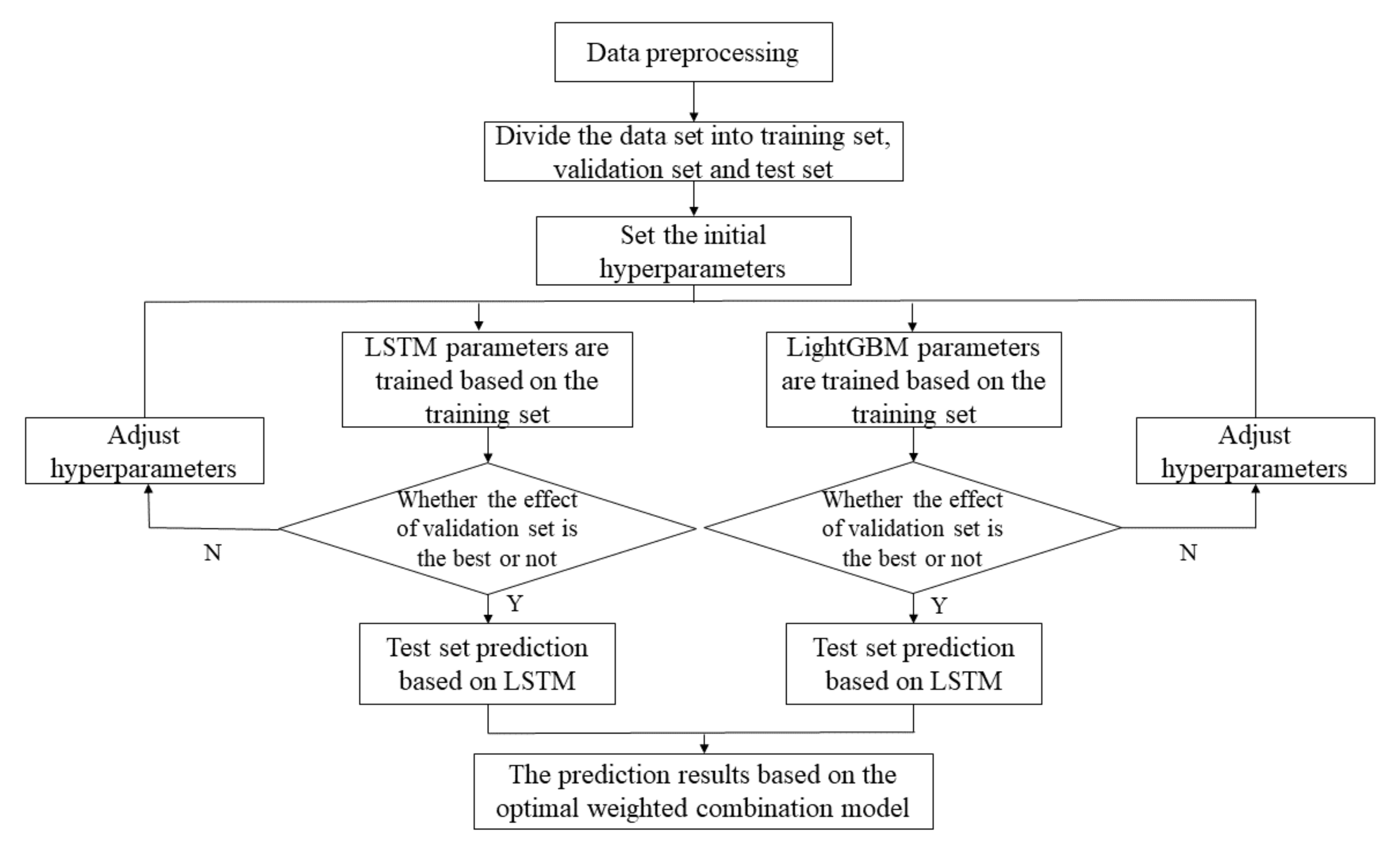
14] adopts the optimal weighting method to determine the weight of each model, which can effectively improve the advantages of a single model. This paper establishes a weighted combination model of LSTM and LightGBM through the optimal weighted combination method based on the residual of the verification set.

2. Model

2.1. LSTM Model

RNNs can process time series data by using neurons with their own feedback. However, as the time series grows, the residual error that RNN needs to return decreases exponentially, resulting in slow update of network weights and the problem of gradient disappearance or gradient explosion. Hochreiter et al. proposed a long-term and short-term neural network [15], replacing the traditional hidden layer with the LSTM layer, which can obtain both the cell state and the hidden layer state from the previous moment. LSTM adopts a control gate mechanism, which is composed of memory cells, input gates, output gates, and forget gates. Its unit structure is shown in Figure 1.
Forget gate: Determine what information the model “forgets” from the cell; ft is the output of the forget gate, the value is between 0 and 1. The closer ft is to 1, the more information is retained in Ct − 1, and the closer ft to 0, the more information is eliminated in Ct − 1. The calculation is shown in Equation (1).
f t = σ W f h t 1 , x t + b f
Input gate: There are two parts of the function, one part is used to find those cell states that need to be updated, and the other part is used to update the information that needs to be updated into the cell state. The calculation is shown in Equation (2):
i t = σ W i h t 1 , x t + b i
Memory unit:
g t = tanh W c h t 1 , x t + b c
C t = f t · C t 1 + i t · g t
Output gate: Determine the information of the output through the sigmoid layer. According to the calculated cell state update value Ct, the output result ht is obtained:
O t = σ W o h t 1 , x t + b o
h t = O t · tanh C t
In Equations (1)–(6), σ represents sigmoid function; Wf, Wi, Wc, and Wo are the weight matrix of forget gate, input gate, memory unit, and output gate, respectively. A vector [ht − 1, xt] is spliced by two vectors; bf, bi, bc, and bo are the bias terms of forget gate, input gate, memory unit, and output gate, respectively; and Ct represents the unit state at the current time and Ct − 1 represents the cell state at the last time.

2.2. LightGBM Model

LightGBM [16] is a distributed gradient boosting framework based on the decision tree algorithm. It still uses the optimization results of (T − 1)-th trees to construct the T-th tree. Each time the combination of weak learners is better than the previous one. Similar to XGBoost, LightGBM explicitly adds a regular term, performs a second-order Taylor expansion of the loss function, and uses first-order and second-order derivative information. The objective function follows:
o b j t = i = 1 n l y i , y ^ i ( t 1 ) + f t ( x i ) + Ω ( f t ) + c o n s tan t
To find ft, make i = 1 n l y i , y ^ i ( t 1 ) + f t ( x i ) + Ω ( f t ) minimum, where Ω(ft) is the regularization term.
GBDT needs to scan all data to estimate all possible segmentation points of information gain, which consumes time and memory. LightGBM uses a GOSS algorithm to reduce samples and an EFB algorithm to bundle features, reducing the time complexity of the algorithm.

2.2.1. Goss Algorithm and EFB Algorithm

First, the GOSS algorithm sorts the samples from large to small based on the absolute value of the gradient, extracts a% samples from the sorted samples, and retains all a% samples. It then randomly samples b% samples from the remaining (1 − a%) samples, in order to maintain the original distribution, amplifies the gradient weights of the [(1 − a%) b%] samples, and multiplies them by (1 − a%)/b%. The new information gain formula follows:
V ˜ J ( d ) = 1 n x i A l g i + 1 a b x i B l g i 2 n l j ( d ) + x i A r g i + 1 a b x i B r g i 2 n r j ( d )
where n is the total number of samples of a node after the Goss algorithm filters samples, n l j d is the number of left samples of the node, and n r j d is the number of right samples of the node.
The EFB algorithm initially constructs a weighted undirected graph using the relationship between features. The nodes are then sorted in descending order according to their degree. The greater the degree, the greater the conflict with other features. Finally, it traverses each feature and assigns it to an existing feature package, or it creates a new feature package to minimize the overall conflict.

2.2.2. Histogram Algorithm

The histogram algorithm [17] greatly improves the efficiency of the LightGBM model, which can discretize the feature sequence and directly support the native support category. It is not necessary to use similar one-hot encoding for feature digitization, as is the case in XGBoost, and transform it into a multidimensional 0/1 feature, which is not efficient in space and time. The histogram algorithm discretizes the floating-point eigenvalues into m integers and builds a histogram with a width of m, as shown in Figure 2 (right). When traversing the data, the discretized value is used as an index to accumulate statistics in the histogram. Once the data are traversed, the histogram will accumulate the required statistics. According to the discrete value of the histogram, the optimal segmentation point is found. Compared with GBDT, traversing all possible segmentation points of each feature to find the optimal segmentation point, LightGBM requires a much smaller memory and greatly improves the speed. The algorithm is shown in Figure 2 [18].
In addition, since the histogram of a leaf can be obtained by the difference between the histogram of its parent node and its brother node, the histogram difference only needs to traverse the k bins of the histogram, and does not need to traverse all the data on this leaf. Therefore, after LightGBM constructs a histogram of a leaf, it can obtain the histogram of its sibling leaves at a very small cost. The “histogram difference acceleration” construction method is shown in Figure 3.

2.2.3. Building the Leafwise Strategy

LightGBM uses the leafwise strategy to split the leaf node with the largest gain among all leaf nodes each time, while limiting the maximum depth of the tree to prevent overfitting. The splitting process is shown in Figure 4 [18].
The splitting gain of a binary tree is shown in Equations (9)–(11) [18].
g a i n = 1 2 G L 2 H L + λ + G R 2 H R + λ ( G L + G R ) 2 H L + H R + λ γ
G j = i I j g i ,     i = 1 , 2 , , n ; j = 1 , 2 , , T
H j = i I j h i ,     i = 1 , 2 , , n ; j = 1 , 2 , , T
where γ is the cost of complexity of introducing new leaf nodes each time, and Gj and Hj are the first and second derivatives of the error function of the sample set.

2.3. Weighted Combination Prediction Model Based on LSTM and LightGBM

2.3.1. An Optimal Weighted Combination Method

LSTM and LightGBM are two completely different models. The former is sensitive to the nature of time series, while the latter has a stronger ability to extract features than the former. There are differences in the predictive abilities of these two models. However, a model with a poor overall forecasting effect does not mean that the model has a bad forecasting ability for all samples. In view of the different advantages of the two models in terms of processing data, this paper combines the models through the optimal weighted combination method, which avoids the overall disadvantage of a single model and improves the stability of the model’s performance. The calculation steps of the optimal weighted combination method follow:
Step 1: Find the deviation matrix E, as shown in Equation (12):
E = i = 1 N e 1 T 2 i = 1 N e 1 T e 2 T i = 1 N e 1 T e 2 T i = 1 N e 2 T 2
where N represents the number of samples contained in the dataset, and e1T and e2T are, respectively, the error between the predicted value and the true value of the LSTM model and the LightGBM model at time T.
Step 2: The optimal weight is obtained by the Lagrange multiplier method, as shown in Equation (13):
[ w 1 , w 2 ] T = E 1 R R T E 1 R
where w1 and w2 are the weight coefficients of the LSTM and LightGBM models, respectively, the sum of the coefficients is 1, and R = [1,1]T.
Step 3: The final PM2.5 concentration prediction result is obtained according to the weight coefficient, as shown in Equation (14):
y ^ T = w 1 y ^ 1 T + w 2 y ^ 2 T
where y ^ T represents the PM2.5 concentration prediction results of LSTM-LightGBM at time T, and y ^ 1 T and y ^ 2 T are the PM2.5 concentration prediction results of the LSTM and LightGBM models, respectively.

2.3.2. The Combined Forecasting Process

The weight coefficients w1 and w2 mentioned in Section 2.3.1 are determined according to the evaluation effect of the validation set. First, the original data are preprocessed, and the training, validation, and test sets are divided according to a certain proportion. According to the evaluation effect of the verification set, the important parameters of the two models are tuned separately, and the test set is used for the actual PM2.5 concentration prediction. After model training and parameter tuning, the test set is independently predicted with LSTM and LightGBM. Finally, the combined prediction result is obtained through the optimal weighted combination method.
The process of combined forecasting is shown in Figure 5.

3. Experimental Setup and Data Processing

3.1. Experimental Environment

The computer configuration used in this experiment follows: an Intel i5-8250 processor, 1.80 Hz CPU frequency, 8 GB memory, and Windows 10 (64-bit) operating system. The software platform is Anaconda (an open source Python distribution for scientific computing), the programming is based on Python 3.7, the LSTM experiment uses the Keras deep learning framework, and the LightGBM model is established based on the LightGBM library.

3.2. Data Source and Index Selection

Marković et al. [19] noted that the sources of PM particles, SO2, NO2, CO, and O3, are different but affect each other. Guo et al. [20] used meteorological factors and other potential pollutant concentrations as the influencing factors of PM2.5 concentration for modeling. This paper selects the hourly historical air quality concentration data and meteorological data of the Beijing Olympic Sports Center from 1 January 2014, to 28 February 2017, in the UCI database, which includes year, month, day, hour, PM2.5 concentration, PM10 concentration, temperature, precipitation, and other information, for a total of 27,720 data and 16 variables, as shown in Table 1. Among them, year, month, day, hour are date-type variables, wd is a subtype variable, and the remaining 11 are all numeric variables. Some data have missing values. This article is concerned with how to predict the concentration of PM2.5 per hour through historical variable information, thus PM2.5 concentration is used as the explained variable, and historical air particulate matter records and weather conditions are used as the explanatory variables.

3.3. Analysis of Influencing Factors of PM2.5 Concentration

3.3.1. Average Concentration of PM2.5 at Different Times

Affected by climatic conditions, the concentration of PM2.5 varies in different seasons. This section explores the changes in the concentration of PM2.5 per hour during the season. According to the climate statistics method, the four seasons are divided into March–May as spring, June–August as summer, September–November as autumn, and December–February as winter. The average concentration of PM2.5 in different months and the hourly average concentration of PM2.5 in different seasons are shown in Figure 6 and Figure 7, respectively.
It can be seen in Figure 6 and Figure 7 that there are differences in PM2.5 at different hours, but it maintains a steady upward or downward trend in similar hours. The PM2.5 concentration is higher in winter, November, and March, and the PM2.5 concentration in summer is significantly lower than the other three seasons. The seasonal concentrations of PM2.5 from high to low follow: winter > autumn > spring > summer. The average concentration of PM2.5 was the highest in December. Because of the severe cold in winter, household coal-fired and carbon-fired heating increase, leading to an increase of pollutants in the air. The trend of PM2.5 concentration in summer and spring is similar. The average concentration of PM2.5 was lowest in August. PM2.5 is higher than other periods from 8 a.m. to 12 a.m., which is caused by the morning peak and factory work; PM2.5 decreases in the afternoon because the temperature at this time limits formation of an inversion layer, which provides greater air circulation and pollutant diffusion; PM2.5 levels increase after 5 p.m. during off-peak hours due to vehicle emissions.

3.3.2. Effects of Air Particulate Matter and Meteorological Factors on PM2.5 Concentration

PM2.5 is a kind of particulate matter affected by other particles in the air and meteorological conditions. The thermal distribution diagram of the correlation between the hourly PM2.5 other air particles and meteorological factors from 1 January 2014 to 28 February 2017 are shown in Figure 8. There is a correlation between them. The other particulate matter in the air has a strong correlation with PM2.5, and meteorological conditions have a weak correlation with PM2.5. Different particulate matter and meteorological conditions have varying degrees of impact on PM2.5.
In terms of air quality, the following conclusions can be made: (1) PM2.5 has the highest correlation with PM10, and its correlation coefficient is as high as 0.88. (2) PM2.5 has a strong positive correlation with SO2, NO2, and CO, and its correlation coefficients are all above 0.7, which shows that harmful pollutants increase the concentration of PM2.5. (3) PM2.5 and O3 are interactive, when the concentration of O3 increases by 1 μg/m3, the concentration of PM2.5 decreases by 0.18 μg/m3 on average, indicating that a certain concentration of O3 is beneficial to suppressing the concentration of PM2.5.
In terms of meteorological conditions, the following conclusions can be made: (1) Wind speed has the greatest impact on PM2.5, and the correlation coefficient is −0.29. (2) PM2.5 is negatively correlated with temperature, rainfall, and wind speed. PM2.5 is suppressed under conditions of high temperature, rainfall, and high wind speed. (3) The dew point temperature and air pressure are positively correlated with PM2.5. The correlation between air pressure and PM2.5 is the smallest, and its correlation coefficient is only 0.0057.

3.4. Data Processing and Division

3.4.1. Data Preprocessing

Missing values and repeated values affect the fitting effect of the model. It is necessary to check whether the dataset contains missing values and duplicate values. It is found that there are no duplicate values in the data, and all other variables except time have missing values. The interpolation method is used to fill numerical variables, and the mode fill method is used to fill subtype variables. The year, month, day, and hour are merged as a data index. Regarding the wind direction of categorized variables, considering that one-hot coding reduces the efficiency of space and time, and the use of one-hot coding cannot have a significant impact on integrated learning; hard coding is used to code it. After the above processing is completed, 12 variables and 27,720 pieces of data are retained.

3.4.2. Data Set Partition and Normalization

Due to the particularity of the time series, the past data are trained to predict the future data, so the dataset cannot be divided randomly. In this paper, in chronological order, the top 70% of the dataset is used as the training set (19,404 data from 1 January 2014, to 19 March 2016), and the middle 20% of the data is used as the validation set (5544 data from 19 March 2016, to 5 November 2016), and the last 10% of the data as a test set (2772 data from 5 November 2016, to 18 February 2017). For each model, it is trained based on the training set, and the verification set is used to select the optimal parameters. Finally, it is predicted on the test set to evaluate the performance of the model. In addition, in order to prevent information leakage, the normalization problem is considered after the dataset is divided.
Since the tree model is optimized by finding the optimal split of the feature, the normalization does not change the position of the split point, so normalization is not required when applying the tree model. However, in order to increase the convergence speed of the NN, when the NN model is established, the data are normalized by minimum–maximum to convert the original data to fall within [0,1]. The normalized expression is shown in Equation (15):
x i j = x i j min 1 i N x i j max 1 i N x i j min 1 i N x i j
where xij represents the original data, xij* is the normalized value, max 1 i N x i j is the maximum value of the selected data feature, and min 1 i N x i j represents the minimum value of the selected data feature. Since the normalized data prediction is not the true predicted value, the conversion factor should be saved to facilitate denormalization after prediction to obtain the actual predicted value. The denormalization method is shown in Equation (16):
y ^ = ( y max y min ) · y ^ + y min
where y ^ is the predicted value of the model with a value [0,1], and y ^ represents the actual predicted value of the model after denormalization.

3.5. Evaluating Indicator

This article explores the problem of regression prediction. It is concerned with whether the predicted PM2.5 is close to the real PM2.5. RMSE, MAE, and SMAPE are selected to measure the prediction accuracy and generalization ability of different models. Let yi be the true value; let y ^ i be the predicted value of the model, i = 1, 2, …, n; and let n be the number of samples. The expressions of the above evaluation indicators are shown in Equations (17)–(19).
R M S E = 1 n i = 1 n y i y ^ 2
M A E = 1 n i = 1 n y ^ i y i
S M A P E = 100 % n i = 1 n y ^ i y i y ^ i + y i / 2
The RMSE and MAE are used to judge the deviation between the predicted value of the model and the true value. The smaller the value, the smaller the prediction error of the model. The SMAPE is used to evaluate the goodness-of-fit of the model, which is an improvement of the mean absolute percentage error (MAPE), which overcomes the asymmetry of MAPE. The closer the value is to 0, the stronger the generalization ability of the model.

4. Model Construction and Evaluation

First, this section establishes the LSTM model and the TSLightGBM model, respectively. According to the performance on the verification set, the two models are weighted by the optimal weighted combination method, and the test set is then predicted. Finally, it is compared with LSTM, TSLightGBM, MLP, RNN, and RF.

4.1. LSTM Model

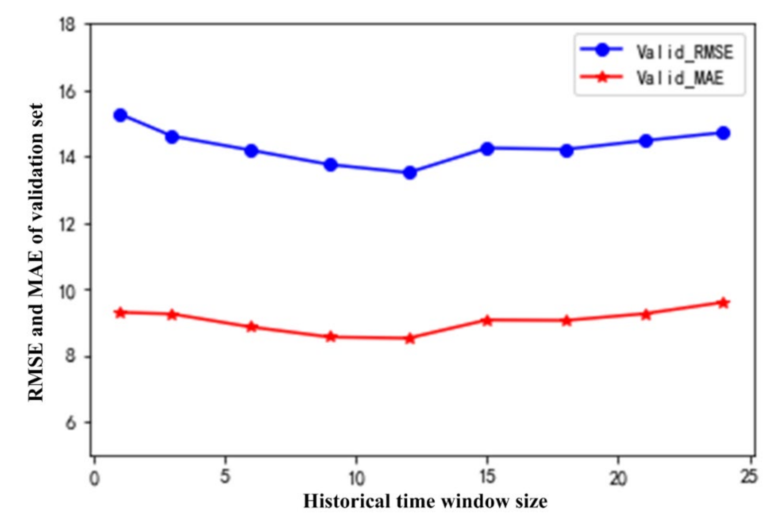
With the continuous accumulation or dissipation of air pollutants over a period of time, the PM2.5 in the air is constantly changing; that is, the PM2.5 in the current period is affected by the influencing factors of the previous N periods. This article conducts comparative experiments by setting different time windows T, where the time window refers to how many hours of historical data are used to predict the current PM2.5. In this paper, the size of the time window is set to 1, 3, 6, 9, 12, 15, 18, 21, and 24.
There are too many parameters affecting the performance of NN. Therefore, first, according to the previous experience, the activation function is determined as ReLU, and the optimization algorithm is determined as the Adam algorithm. Two hidden layers are set, the learning rate is set as the default parameter of 0.01, and some neurons are randomly deleted with a probability of 0.2. A pre-experiment is set to roughly adjust the secondary important parameters. In the pre-experiment, the batch size is set as 16, 32, and 64, the number of iterative training epochs is set to 100 and 200 to model the training samples, two hidden layers are set, the batch is set to 32, and the number of epochs is set to 100, which is more appropriate. At the same time, the MAE of the verification set has an upward trend in the last 50 trainings, so a mechanism (Early_Stopping) is set to prevent the model from overfitting. When the MAE of the verification set decreases by no more than 0.0005 for 15 consecutive times, model training is considered complete. According to the previous experience, the parameter settings completed by the pre-experiment are shown in Table 2.
The formal experiment mainly adjusts the number of neurons contained in the two hidden layers. Under different time windows T, these two parameters must be continuously adjusted. The MAE is used as an evaluation index, and the parameter corresponding to the minimum MAE of the verification set in the current time window is selected. According to the length of the input sequence, the number of neurons in the hidden layer is obtained within the range of [50,400]. The optimal parameter settings obtained under each time window and the MAE and RMSE of the verification set are shown in Table 3. Considering the authenticity of the results of the verification set, the MAE and RMSE in Table 3 are calculated based on the index formula after restoring the predicted value of the verification set.
As shown in Table 3, when T = 12, LSTM performs best on the validation set. The MAE and RMSE are 8.522 and 13.515, respectively. When T = 24, LSTM performs the worst on the validation set; MAE and RMSE are 9.604 and 14.724, respectively. In order to more intuitively judge the relationship between the prediction ability of LSTM and the size of T, the effect of the verification set of LSTM under each time window is presented in Figure 9.
In Table 3 and Figure 9, as the time series increases, the overall performance of LSTM on the PM2.5 value shows an upward trend and then a downward trend. The effect on the verification set is best when T = 12. The LSTM model has similar prediction performance for PM2.5 within 3 h. For example, when T = 1 and T = 3, the MAE and RMSE are about 9.27 and 14.9, respectively; when T = 9 and T = 12, the MAE and RMSE are about 8.5 and 13.5, respectively; and when T = 15 and T = 18, the MAE and RMSE are about 9.05 and 14.2, respectively.
In summary, when the T is set to 12, LSTM performs best on the verification set. The specific parameters follow: the activation function is set to ReLU, the optimization algorithm is the Adam algorithm, the learning rate is the default parameter of 0.01, the batch size is 32, and the number of neurons in the first and second hidden layers is set to 320 and 160, respectively. During training, each hidden layer randomly discards some neurons with a probability of 0.2. If the MAE of the validation set drops less than 0.0005 for 15 consecutive times, training stops.

4.2. The TSLightGBM Model

When integrated models such as LightGBM and RF process time series, there is no time correlation between the input data. There are generally two ways to introduce time features: (1) One is to add basic feature variables, such as year, season, month, week, and hour. This model is denoted as TLightGBM. (2) The other uses T as a sliding window, and statistics such as the mean and standard deviation of each samples’ features are used as feature variables before T hours, so as to introduce the time characteristics to improve the training accuracy of the model. This model is denoted as TFLightGBM in this paper. However, these two methods do not make full use of the data in the time window T, and some information will be lost. In this section, when the time window size T is selected, the data of each T period are spliced into a one-dimensional shape as the explained variable of the PM2.5 of the T + 1 period, so as to predict the PM2.5 of the T + 1 h. In this paper, this model is denoted as TSLightGBM and compares it with the previous two methods that introduce temporal features. In order to ensure the fairness of the model comparison, the size of the selected sliding window and time window are the same as in Section 4.1.
Considering that there are many parameters of the LightGBM model, the ensemble model of the tree is mainly affected by the number of trees, the maximum depth, and the learning rate. This section mainly adjusts the three main parameters of LightGBM as minimally as possible with the goal of verifying the set MAE. The number of trees (n_estimators) is adjusted within [100, 250, 500, 1000, 2000], the maximum tree depth (max_depth) is adjusted within [6, 8, 10, 12, 16], and the learning rate (learning_rate) is adjusted within [0.01, 0.05, 0.1]. The final adjustment results and the corresponding MAE and RMSE values are shown in Table 4.
Table 4 shows the following: (1) The model with the best effect is TSLightGBM, and its RMSE and MAE are 8.153 and 13.266, respectively; (2) the second-best model is TLightGBM, and its RMSE and MAE are 12.496 and 19.570, respectively; and (3) the worst model is TFLightGBM, and its RMSE and MAE are 18.180 and 26.796, respectively. When LightGBM cannot provide the input data with a time correlation, the data in T are spliced into a one-dimensional shape as an explanatory variable to predict PM2.5 in the T + 1 period, and the prediction performance of the model is better.
In summary, the feature construction method of TSLightGBM is selected, the number of trees is set to 1000, the maximum depth of the tree is 10, and the learning rate is 0.01. LightGBM performs best on the verification set.

4.3. LSTM-TSLightGBM Weighted Combination Model

Based on the verification set MAE of the optimal LSTM and the optimal LightGBM in Section 4.1 and Section 4.2, the ratio (0.42:0.58) of two models in the prediction is calculated according to the optimal weighted combination method.
In order to better evaluate the performance of the combined model, this section compares it with MLP, RNN, RF, LSTM, and TFLightGBM. These models all choose the parameters with the goal of the smaller MAE of the validation set. Among them, the input of MLP and RF is similar to that of TFLightGBM. Similar to other NNs, MLP is normalized when training the model. The RNN is constructed in the same way as LSTM. The real prediction performance of each model is shown in Table 5.
Table 5 shows the following: (1) the weighted combination model LSTM-TSLightGBM has a better performance than any single model, and its MAE, RMSE, and SMAPE are the smallest, which are 11.873, 22.516, and 19.540%, respectively; (2) the second-best model is TSLightGBM, and its MAE, RMSE, and SMAPE are 12.278, 23.216, and 19.936%, respectively; (3) the third-best model is LSTM. Although the SMAPE of LSTM is 0.321% larger than that of RF, its MAE and RMSE are 12.918 and 23.501 respectively, which are 0.1 and 1.2 smaller than that of RF. Overall, LSTM is a better model than RF.
This paper assumes that if the difference between the prediction errors of the two models exceeds 10%, it is considered that there is a significant difference in the prediction performance of the two models. Compared with MLP and RNN models, MAE of LSTM-TSLightGBM decreased by 33.50% and 29.52%, respectively; RMSE decreased by 19.75% and 17.09% respectively; and SMAPE decreased by 47.15% and 44.94% respectively. On the whole, the prediction effect of LSTM-TSLightGBM on PM2.5 concentration is significantly improved.
To more intuitively judge the superiority of the LSTM-TSLightGBM performance, it is necessary to further combine graphics to judge its performance. Considering that the effect of graphic display is not obvious when the difference degree of MAE is within 1, this section only shows the comparison curve between the predicted value and the real value of LSTM-TSLightGBM model with the best performance and the MLP model with the worst performance. Due to the large sample size of the test set, all visualization will affect the judgment effect. Here, 100 samples are drawn from the first and second halves of the test set for comparison. The visualization results are shown in Figure 10 and Figure 11.
As shown in Figure 10 and Figure 11, compared with the LSTM-TSLightGBM model, the difference between the predicted value of MLP neural network and the actual value is more obvious. When PM2.5 is in the range of 100 to 200, the predictive capabilities of LSTM-TSLightGBM and the MLP neural network are close. However, when PM2.5 is close to 0 or greater than 350, the difference between the predicted value of MLP and the real value is clear, while the difference between the LSTM-TSLightGBM model and the real value is not. The reason why LSTM-TSLightGBM is better may be that LSTM has a “memory” function, and the variable inputs to the MLP are independent of each other. In addition, LSTM has gating rules and selectively filters variable information. At the same time, TSLightGBM also has the function of screening variables, which can reduce the influence of noise.
In terms of evaluation indicators and prediction results, LSTM-TSLightGBM combines the advantages of LSTM’s high sensitivity to time information and the advantages of LightGBM’s strong extraction of feature variables. Therefore, LSTM-TSLightGBM has superiority in the prediction of PM2.5.

5. Conclusions

Based on the hourly historical air quality data and meteorological dataset from the environmental monitoring site of the Beijing Olympic Sports Center from 1 January 2014, to 28 February 2017, this paper conducts an empirical study and draws the following conclusions:
(1)
The overall seasonal variation of PM2.5 concentration, from highest to lowest, shows the following pattern: winter > autumn > spring > summer. The average concentration of PM2.5 is highest in December and the lowest in August. The concentration of PM2.5 is positively correlated with the concentration of harmful particulate matter. The correlation between PM2.5 and PM10 is the highest, reaching 0.88. A certain concentration of O3 is conducive to suppressing the concentration of PM2.5, and high temperature, rainfall, and wind speed have a certain inhibitory effect on PM2.5. Meteorological factors have a small impact on PM2.5.
(2)
As the PM2.5 concentration is affected by historical information, the performance of LSTM is related to the size of the time window. As the time window increases, the performance of LSTM on PM2.5 increases first and then decreases. When the time window size is 12, performance of LSTM is best. For the nontime series model, LightGBM, different feature construction methods have an impact on the performance. The TSLightGBM, which uses all the information in the time window as the input the next period of prediction, has the best performance.
(3)
Comparing LSTM-TSLightGBM with LSTM, TSLightGBM, RF, RNN, and MLP neural networks, LSTM-TSLightGBM has the smallest MAE, RMSE, and SMAPE, which demonstrates its effectiveness in processing time series data and its superiority in the hourly forecast of PM2.5.

Author Contributions

Conceptualization, X.J. and Y.L.; methodology, Y.L. and X.J.; formal analysis, X.J. and Y.L.; data curation, B.Z.; funding acquisition, B.Z. and X.J.; supervision, B.Z.; writing—original draft preparation, Y.L. and X.J.; writing—review and editing, Y.L. and B.Z. All authors have read and agreed to the published version of the manuscript.

Funding

The research is supported by the Natural Science Foundation of Hubei Province, China (Grant No. 2020CFB180). The authors are grateful to other participants of the project for their cooperation.

Institutional Review Board Statement

Not applicable.

Informed Consent Statement

Not applicable.

Data Availability Statement

Data and methods used in the research are presented in sufficient detail in the paper.

Conflicts of Interest

The authors declare no conflict of interest.

References

  1. Wang, P.; Zhang, H.; Qin, Z.; Zhang, G. A novel hybrid-Garch model based on ARIMA and SVM for PM2.5 concentrations forecasting. Atmos. Pollut. Res. 2017, 8, 850–860. [Google Scholar] [CrossRef]
  2. Yu, H.; Yuan, J.; Yu, X.; Zhang, L.; Chen, W. Tracking prediction model for PM2.5 hourly concentration based on ARMAX. J. Tianjin Univ. Sci. Technol. 2017, 50, 105–111. [Google Scholar]
  3. Kanirajan, P.; Kumar, V.S. Power quality disturbance detection and classification using wavelet and RBFNN. Appl. Soft Comput. 2015, 35, 470–481. [Google Scholar] [CrossRef]
  4. Chen, S.; Wang, J.; Zhang, H. A hybrid PSO-SVM model based on clustering algorithm for short-term atmospheric pollutant concentration forecasting. Technol. Forecast. Soc. Chang. 2019, 146, 41–54. [Google Scholar] [CrossRef]
  5. Biancofiore, F.; Busilacchio, M.; Verdecchia, M.; Tomassetti, B.; Aruffo, E.; Bianco, S.; Di Tommaso, S.; Colangeli, C.; Rosatelli, G.; Di Carlo, P. Recursive neural network model for analysis and forecast of PM10 and PM2.5. Atmos. Pollut. Res. 2016, 8, 652–659. [Google Scholar] [CrossRef]
  6. Tsai, Y.T.; Zeng, Y.R.; Chang, Y.S. Air pollution forecasting using RNN with LSTM. In Proceedings of the 2018 IEEE 16th Intl Conf on Dependable, Autonomic and Secure Computing, 16th Intl Conf on Pervasive Intelligence and Computing, 4th Intl Conf on Big Data Intelligence and Computing and Cyber Science and Technology Congress (DASC/PiCom/DataCom/CyberSciTech), Athens, Greece, 12–15 August 2018; IEEE: Piscataway, NJ, USA, 2018; pp. 1074–1079. [Google Scholar]
  7. Liu, W.; Guo, G.; Chen, F.; Chen, Y. Meteorological pattern analysis assisted daily PM2.5 grades prediction using SVM optimized by PSO algorithm. Atmos. Pollut. Res. 2019, 10, 1482–1491. [Google Scholar] [CrossRef]
  8. Sun, W.; Sun, J.S. Daily PM2.5 concentration prediction based on principal component analysis and LSSVM optimized by cuckoo search algorithm. J. Environ. Manag. 2017, 188, 144–152. [Google Scholar] [CrossRef] [PubMed]
  9. Zhao, W.; Xia, L.; Gao, G.; Cheng, L. PM2.5 prediction model based on weighted KNN-BP neural network. J. Environ. Eng. Technol. 2019, 9, 14–18. [Google Scholar]
  10. Liu, X.; Zhao, W.; Tang, W. Forecasting Model of PM2.5 Concentration one Hour in Advance Based on CNN-Seq2Seq. J. Chin. Comput. Syst. 2020, 41, 1000–1006. [Google Scholar]
  11. Kow, P.Y.; Wang, Y.S.; Zhou, Y.; Kao, F.-I.; Issermann, M.; Chang, L.-C.; Chang, F.-J. Seamless integration of convolutional and back-propagation neural networks for regional multi-step-ahead PM2.5 forecasting. J. Clean. Prod. 2020, 261, 121285. [Google Scholar] [CrossRef]
  12. Guo, C.; Guo, W.; Chen, C.H.; Wang, X.; Liu, G. The air quality prediction based on a convolutional LSTM network. In Proceedings of the International Conference on Web Information Systems and Applications, Qingdao, China, 20–22 September 2019; Springer: Cham, Switzerland, 2019; pp. 98–109. [Google Scholar]
  13. Zhang, Y.; Yuan, H.; Sun, X.; Wu, H.; Dong, Y. PM2.5 Concentration Prediction Method Based on Adam’s Attention Model. J. Atmos. Environ. Opt. 2021, 16, 117. [Google Scholar]
  14. Weng, T.; Liu, W.; Xiao, J. Supply chain sales forecasting based on lightGBM and LSTM combination model. Ind. Manag. Data Syst. 2019, 120, 249–265. [Google Scholar] [CrossRef]
  15. Hochreiter, S.; Schmidhuber, J. Long short-term memory. Neural Comput. 1997, 9, 1735–1780. [Google Scholar] [CrossRef] [PubMed]
  16. Ke, G.; Meng, Q.; Finley, T.; Wang, T.; Chen, W.; Ma, W.; Ye, Q.; Liu, T.-Y. LightGBM: A Highly Efficient Gradient Boosting Decision Tree. In Proceedings of the 31st Conference on Neural Information Processing Systems (NIPS 2017), Long Beach, CA, USA, 4–7 December 2017. [Google Scholar]
  17. Dale-Jones, R.; Tjahjadi, T. A study and modification of the local histogram equalization algorithm. Pattern Recognit. 1993, 26, 1373–1381. [Google Scholar] [CrossRef]
  18. Wang, Y.; Wang, T. Application of improved LightGBM model in blood glucose prediction. Appl. Sci. 2020, 10, 3227. [Google Scholar] [CrossRef]
  19. Marković, D.M.; Marković, D.A.; Jovanović, A.; Lazić, L.; Mijić, Z. Determination of O3, NO2, SO2, CO and PM 10 measured in Belgrade urban area. Environ. Monit. Assess. 2008, 145, 349–359. [Google Scholar] [CrossRef] [PubMed]
  20. Guo, J.; Xia, F.; Zhang, Y.; Liu, H.; Li, J.; Lou, M.; He, J.; Yan, Y.; Wang, F.; Min, M.; et al. Impact of diurnal variability and meteorological factors on the PM2. 5-AOD relationship: Implications for PM2. 5 remote sensing. Environ. Pollut. 2017, 221, 94–104. [Google Scholar] [CrossRef] [PubMed] [Green Version]
Figure 1. LSTM cell structure.
Atmosphere 12 01211 g001
Figure 2. Histogram algorithm.
Atmosphere 12 01211 g002
Figure 3. “Histogram difference acceleration” construction method.
Atmosphere 12 01211 g003
Figure 4. Tree building diagram based on the leafwise strategy.
Atmosphere 12 01211 g004
Figure 5. Flow chart of combined forecasting.
Atmosphere 12 01211 g005
Figure 6. Average concentration of PM2.5 in different months.
Atmosphere 12 01211 g006
Figure 7. Average PM2.5 concentration per hour in different seasons.
Atmosphere 12 01211 g007
Figure 8. Thermal distribution diagram of correlation between air particulate matter, meteorological factors, and PM2.5.
Atmosphere 12 01211 g008
Figure 9. The RMSE and MAE of the LSTM verification set under different time windows.
Atmosphere 12 01211 g009
Figure 10. LSTM-TSLightGBM prediction results: (a) 100 random samples in the first 50% of the test set, (b) 100 random samples in the last 50% of the test set.
Atmosphere 12 01211 g010
Figure 11. MLP neural network prediction results: (a) 100 random samples in the first 50% of the test set, (b) 100 random samples in the last 50% of the test set.
Atmosphere 12 01211 g011
Table 1. Variable description.
VariableMeaningVariableMeaning
YearYear of this rowCOCO concentration (μg/m3)
MonthMonth of this rowO3O3 concentration (μg/m3)
DayDay of this rowTEMPTemperature (°C)
HourHour of this rowPRESPressure (hPa)
PM2.5PM2.5 concentration (μg/m3)DEWPDew point Temperature (°C)
PM10PM10 concentration (μg/m3)RAINPrecipitation (mm)
SO2SO2 concentration (μg/m3)WDWind direction
NO2NO2 concentration (μg/m3)WSPMWind speed (m/s)
Table 2. Parameter settings.
ParametersSetting
Activation functionReLU
Optimization algorithmAdam
Learning rate0.01
Discard rate0.2
Batch parameters32
Early stop mechanismIf the MAE of the verification set drops less than 0.0005 for 15 consecutive times, training is stopped
Table 3. The parameter setting and verification effect under different time windows.
TNumber of Neurons in the First LayerNumber of Neurons in the Second LayerMAERMSE
1100509.30015.287
3120609.25214.619
6128648.86014.192
92561288.55713.760
123201608.52213.515
153001509.07314.258
183001509.05814.219
212561289.26014.480
243501759.60414.724
Table 4. The final adjustment results of LightGBM and the corresponding MAE and RMSE.
Modeln_estimatorsmax_depthlearning_rateMAERMSE
TLightGBM100060.0112.49619.570
TFLightGBM2000100.0118.18026.796
TSLightGBM1000100.018.15313.266
Table 5. The performance of each model.
ModelMAERMSESMAPE
MLP17.85328.05836.974%
RNN16.84627.15835.487%
RF13.02724.70220.950%
LSTM12.91823.50121.271%
TSLightGBM12.27823.21619.936%
LSTM-TSLightGBM11.87322.51619.540%
Publisher’s Note: MDPI stays neutral with regard to jurisdictional claims in published maps and institutional affiliations.

