A Haze Prediction Method Based on One-Dimensional Convolutional Neural Network

Abstract

In recent years, more and more people are paying close attention to the environmental problems in metropolitan areas and their harm to the human body. Among them, haze is the pollutant that people are most concerned about. The demand for a method to predict the haze level for the public and academics keeps rising. In order to predict the haze concentration on a time scale in hours, this study built a haze concentration prediction method based on one-dimensional convolutional neural networks. The gated recurrent unit method was used for comparison, which highlights the training speed of a one-dimensional convolutional neural network. In summary, the haze concentration data of the past 24 h are used as input and the haze concentration level on the next moment as output such that the haze concentration level on the time scale in hours can be predicted. Based on the results, the prediction accuracy of the proposed method is over 95% and can be used to support other studies on haze prediction.

1. Introduction

Haze is one of the most harmful air pollutants to the human body as it can directly enter the lungs and cause harm [1]. Compared with other kinds of air pollutants, haze is a more recent concern for human society. In recent years, more and more people are paying close attention to the environmental issues in metropolitan areas and their impact on the human body. Among them, haze is the air pollutant that people are most concerned about. Haze is a weather phenomenon that is closely related to social development and industrialized urbanization [2], which means it would affect high population-concentrated urban and factory areas. However, due to the complexity of the atmosphere and that the components of haze are very sensitive to changes in atmospheric conditions, the study of haze, especially the prediction of haze, has been difficult.

With the development of machine learning and neural network technology [3,4,5,6,7,8], neural networks have been widely used in environmental science, including all kinds of natural hazards [9,10,11,12,13,14]. In the past century, many researchers abroad have used some neural network knowledge to process atmospheric pollutant data. For example, in 1998, researchers such as Hubbard conducted regression analysis on atmospheric pollutant ozone concentration and made certain predictions [15]. In 2000, Pérez P and other researchers [16] used the structure of the neural network to predict and analyze the average concentration of haze in the San Diego area in the next few hours. In 2006, researchers such as Grivas [17] optimized the structure and parameters of neural networks based on the previous study of Pérez to predict the concentration of PM10. In addition, with continuous optimization of the network, many scholars have used neural networks to predict and analyze the haze on a time series [18,19,20].

Similarly, much research has been on the problem of haze conducted in China [21,22,23]. Sun et al. [24] analyzed the chemical characteristics of different PM during a Beijing haze. By treating the year-to-year increment as predicted, Yin et al. [25] established two new statistical schemes using multiple linear regression (MLR) and the generalized additive model (GAM), which both had higher predictive skills.

In the application of convolutional neural networks to weather phenomena, Shi et al. [26] proposed a convolution LSTM (long short-term memory) method in 2015 to extract features from radar signals. The network is input in chronological order, and the prediction of future rainfall is realized due to the existence of the LSTM network relationship. Although this model is not used for the research and analysis of haze, it does demonstrate that convolutional neural networks can be used to predict and analyze weather phenomena. At the 2015 Conference on Computer Vision and Pattern Recognition (CVPR), Klein et al. [27] proposed a ‘systematic convolutional layer’ for forecasting weather phenomena. Due to the complexity of haze and atmospheric conditions, this paper aims to propose a simple yet efficient method to provide near-future haze level prediction that could be used to support information for other related studies.

In this paper, one-dimensional haze time series data were used as input and the haze concentration level at the next moment was used as output to train a one-dimensional convolutional neural network (1D-CNN) to achieve the haze concentration prediction at the next moment. The 1D-CNN is compared with other methods to evaluate if it is suitable for the proposed task. Then, a one-dimensional convolutional neural network based on special calibration is proposed to extract features on the time dimension to achieve the prediction of the haze concentration level at the next moment.

2. Materials

The one-dimensional data used in this paper were derived from the data published by Peking University on the Machine Learning Repository. The data set is used for machine learning processing and contains 13 variables (row, year, month, day, hour, PM2.5, DEWP, TEMP, PRES, CBWD, LWS, IS, IR) with a time range from 1 January 2010 to 31 December 2014, for a total of five years, as well as the average concentration of haze, air pressure, temperature, wind speed, and wind direction.

Only the PM2.5 data in the experiments were used as the data for studying haze.

The input was calibrated using the concentration level at the next moment of the input time period. This trains the one-dimensional convolutional neural network to predict the next moment of smog. For the classification of the concentration, we used the grading method of average division, and divided it into ten grades according to smog concentration, as shown in the

Table 1. Detailed haze concentration level table.

Level	1	2	3	4	5	6	7	8	9	10
Concentration	35	70	105	140	175	210	245	280	315	500

:

The method for data calibration as Equation (1):

$$y_i=[\begin{array}{cccc}{c}_1& c_2& \dots & c_{10}\end{array}]$$

(1)

where $y$ is a one-hot vector.

3. Methodology

Convolutional neural networks have been widely used in image data processing [28,29,30,31], natural language processing [32,33], mechanical research [34,35,36], and other fields.

However, with the deepening of research, researchers have found that the convolutional neural network has unique advantages in the processing of one-dimensional signals [37,38,39].

In this section, we use the one-dimensional time series data of haze as the input and the level of haze concentration at the next moment as the output to train the one-dimensional convolutional neural network to realize the prediction of haze concentration at the next moment.

$x_{in}\in R^n$ represents the input haze time series data with a length of n. $y\in R^{10}$ represents the corresponding haze concentration level output, which is a vector of length 10. The learning goal of the one-dimensional convolutional neural network is the nonlinear mapping between the haze time series and the haze concentration level for the next time period from input to output as Equation (2):

$$y_{out}=F\left(x_{in}\right)$$

(2)

where F is represents a complex nonlinear mapping relationship between input data and output markers. In order to better express this complex mapping relationship, in this section, we transform the haze time series prediction problem into the mean square error function to find the minimum set in order to minimize the difference between the relationship fitted to the mapping function F and the real relationship as Equation (3):

$$L=\underset{F}{argmin}{\parallel y_{out}\left(x\right)-F\left(x\right)\parallel }_2^2$$

(3)

This method is the process of minimizing the difference between the output and the calibrated output. That is, the process by which the neural network adjusts the parameters.

Assume that the multilayer convolutional neural network used in this section has a total of I. For the i-th convolutional layer, the input $a_{i-1}$ is the output of the upper layer, and the output of the i-th layer is as Equation (4):

$$a_i=f_i\left(a_{i-1}\right)=\sigma \left(W_i{a}_{i-1}+b_i\right)$$

(4)

where $\sigma$ is the nonlinear activation function and $W_i$ is the weight in the convolution kernel. $b_i$ is the amount of offset added after convolution for a better nonlinear fitting. If the i-th layer is a convolutional layer, the activation function selects the rectified linear unit (ReLU) function. If the i-th layer is a fully connected layer, the activation function used in this layer is selected as the sigmoid function. This allows the nonlinear relationship between input and output to be expressed as Equation (5):

$$F\left(x_{in}\right)=f_l\left(f_{l-1}\left(\dots f_1\left(x_{in}\right)\right)\right)$$

(5)

The last layer is the classification layer, which performs soft max multiclassification, back propagates the error between the output and the calibration output, and then adjusts the optimization parameters so that the mean square error difference between them is minimized. In this way, the input data are convolved, pooled, fully connected, and multiclassified in the one-dimensional convolutional neural network and, finally, the feature extraction and prediction of the haze in time series is realized.

The general structure of a one-dimensional convolutional neural network is shown in Figure 1. It consists of five parts: a one-dimensional input layer, a one-dimensional convolutional layer, a one-dimensional pooling layer, a fully connected layer, and a classification layer. Different from the two-dimensional convolutional neural network structure, all convolution kernels and the pooled layer structure are also one-dimensional.

(1)

Convolution process of one-dimensional convolution network: In a one-dimensional convolutional neural network, the convolution of the first layer can be regarded as an operational relationship between the weight vector $W\in R^m$ and the input vector $x_{in}\in R^n$. The weight vector has a size of m, that is, the size of the convolution kernel is m. More specifically, $x_{in}$ is the haze period vector as output, and each of the elements is a haze concentration value at a time point. The convolution kernel of m size is used to convolve the sequence of each m length in the input vector to obtain the output of the first layer. Where $m\ll n$, this ensures that the haze concentration value at each moment in the input is included in the convolution operation. If the step size is 1, the convolution formula is as follows:

$$a_i={\mathit{x}}_{i:i+m-1}{W}^T$$

(6)

(2)

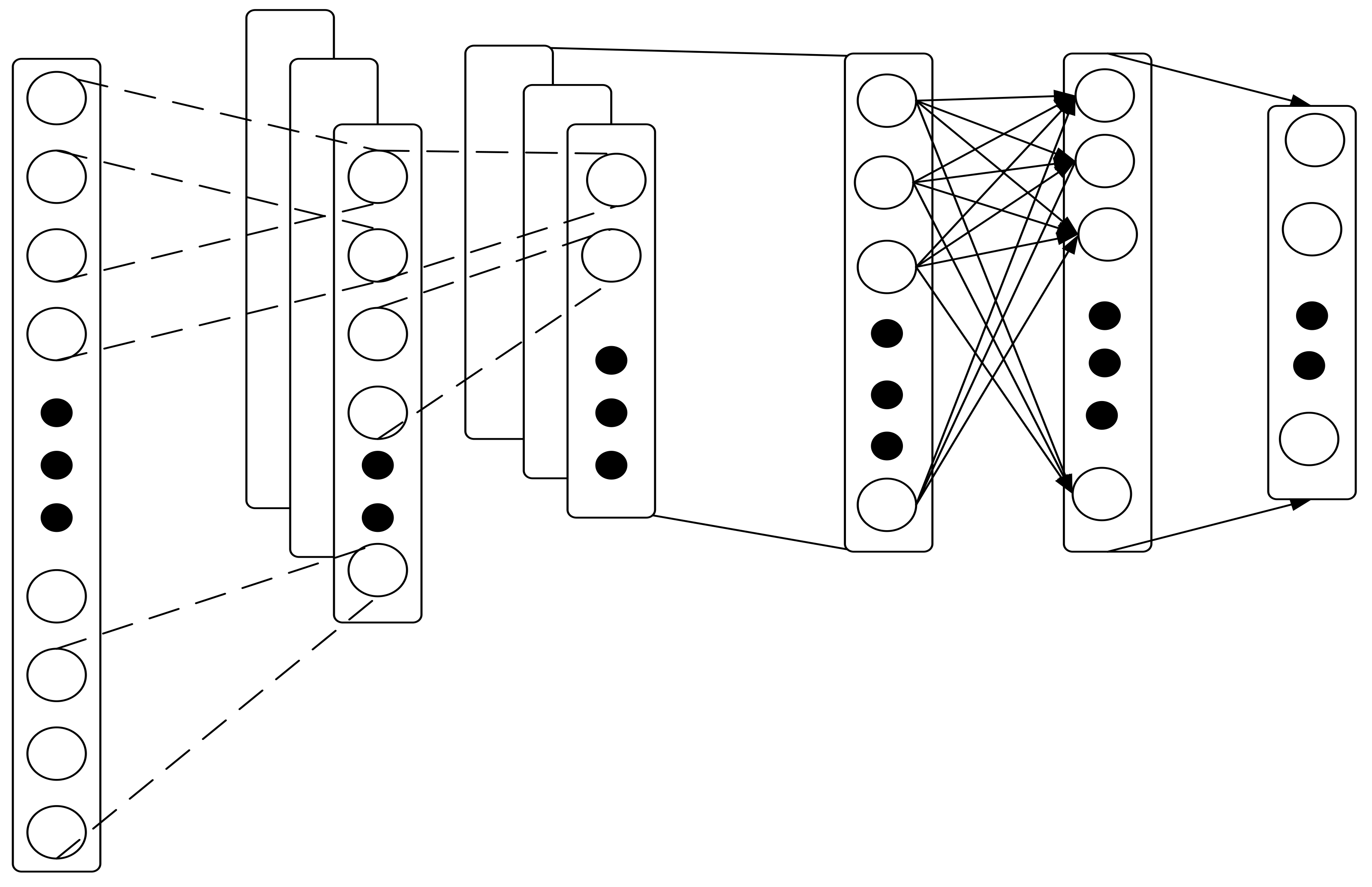
One-dimensional convolution layer: Since the one-dimensional convolution input layer is a one-dimensional vector, its convolution kernel is also one-dimensional. To illustrate the convolution process more specifically, a one-dimensional convolution process with an input length of 7, a convolution kernel size of 5, and a convolution step of one is shown in Figure 2.

(3)

One-dimensional convolution pooling layer: Due to the existence of the pooling layer, the one-dimensional convolutional neural network also fully exerts the neural network in theory due to the feature extraction, which can be equivalent in theory. The training speed of one-dimensional convolutional neural networks is inherently superior to other neural networks.

Since the data used in this experiment are time series, the testing method is walk forward validation [40,41]. A minimum number of observations is selected for training in the prediction of next time step. The prediction result will be compared to the known value of the next time step so that the prediction is evaluated. The window of the minimum observation will move to include the known value to make a prediction of the following time step, and then the process is repeated.

4. Experiments and Results

4.1. Comparison of 1D Convolutional Neural Network and GRU Circulatory Neural Network

A set of experiments is used in this section to demonstrate the advantages of one-dimensional convolutional neural networks in processing one-dimensional data. In this experiment, this section selects the gated recurrent unit (GRU) [42] cyclic neural network widely used in one-dimensional signal processing for comparison. According to the idea of control variables, the data in this section selects Benchmark, the standard data training library, to compare the performance of the two networks. The advantages of one-dimensional convolutional neural networks are analyzed by experiments on the same data by two networks.

The comparison network uses a GRU neural network. The method of processing sequence data is as follows:

• The input of the front layer and the input of this unit are weighted and then passed through an activation function to obtain an alternative value.
• Then, the input of the same front layer and the input of this unit are subjected to the same weighting, and the sigmoid activation function is mapped to 0, 1. This mapping value is the update gating parameter.
• Determine whether the parameter is updated by a gate control unit. By changing the relationship between the hidden layers of the cyclic neural network, the problem of weak correlation before and after the sequence input is solved.

The standard database (Benchmark) training set used in this section has 50,000 pieces of data. The following is the time used by the two networks to process these data, and the set learning rate is 0.0001. Then, the maximum number of iterations epoch is specified as 10 rounds, and the number of iterations per round is 400. The training result is displayed after every 100 iterations, and the result is saved once after 10 iterations. If the training result of the 100 iterations is better than the result of the last 100 iterations, it means that the training is effective. As per training termination conditions, the training is terminated if the accuracy is not improved after ten rounds of training or 500 iterations.

Training conditions: The computer processor model used during the training of the two networks is Intel Core i7-4790. The total training time of 1600 rounds of one-dimensional convolutional neural network is 29 min and 17 s, while the time required for 2200 rounds of GRU network training is 3 h, 47 min and 28 s.

Through experiments, the accuracy of the one-dimensional convolutional neural network and the GRU circular neural network in different iterations is shown in the Figure 3 and Figure 4:

The following conclusions can be drawn from the training process:

(1)

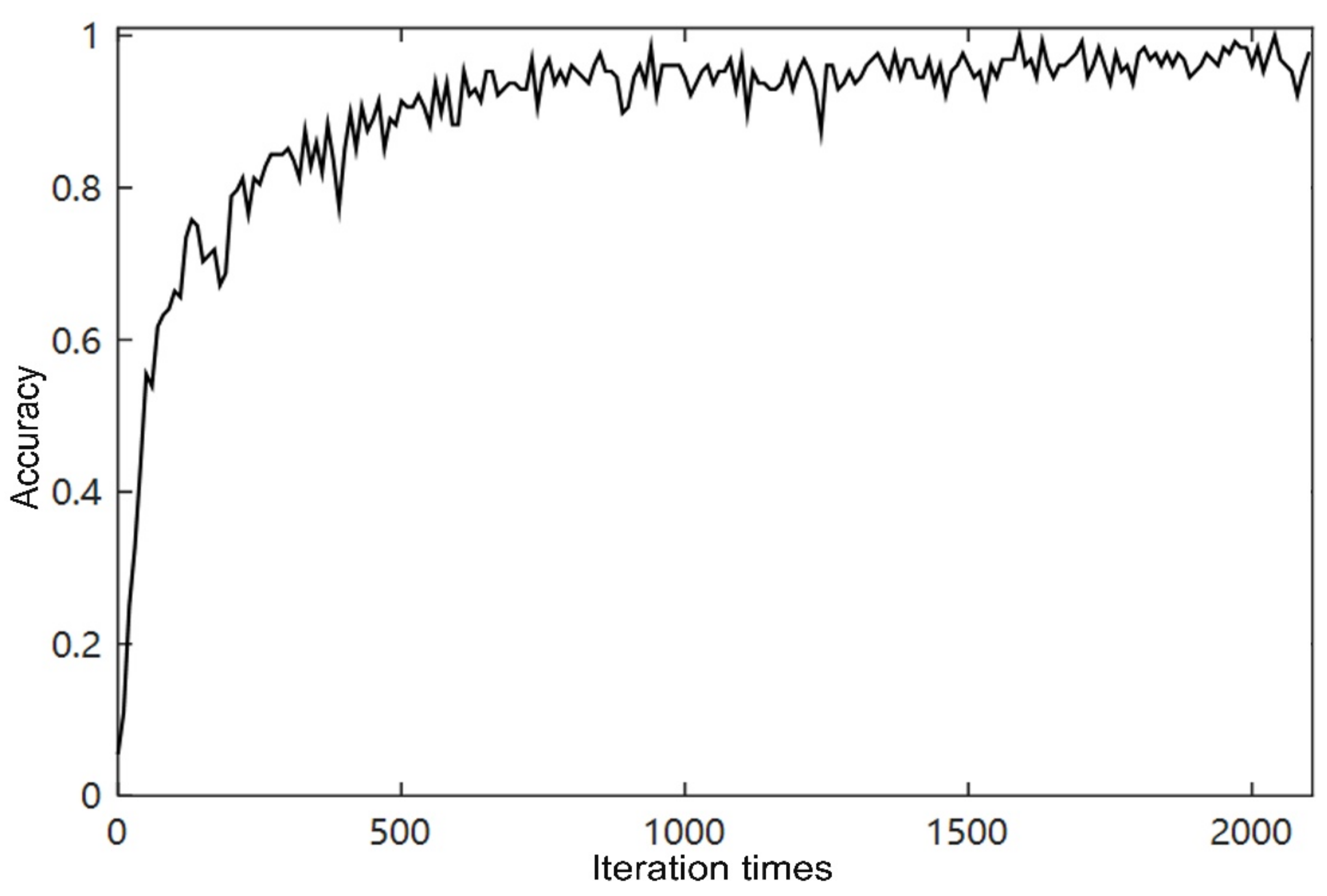
Convolution: The number of iterations required for the neural network to achieve the best accuracy is less than that of the cyclic neural network. The convolutional neural network stops after 1600 iterations, and the cyclic neural network only achieves the optimal result as specified by us at the 2200th iteration.

(2)

Due to the characteristics of weight sharing and the local connection of the convolutional neural network, the training speed of the convolutional neural network is faster. The time for the convolutional neural network is about 120 s per 100 iterations, while the cyclic neural network is every 100 iterations. The time required is about 600 s.

(3)

Overall, although the initial accuracy of GRU increases slower than the one-dimensional convolutional neural network, optimization results continue to appear as the rounds increase. After more rounds of training, the GRU recurrent neural network can also obtain better results.

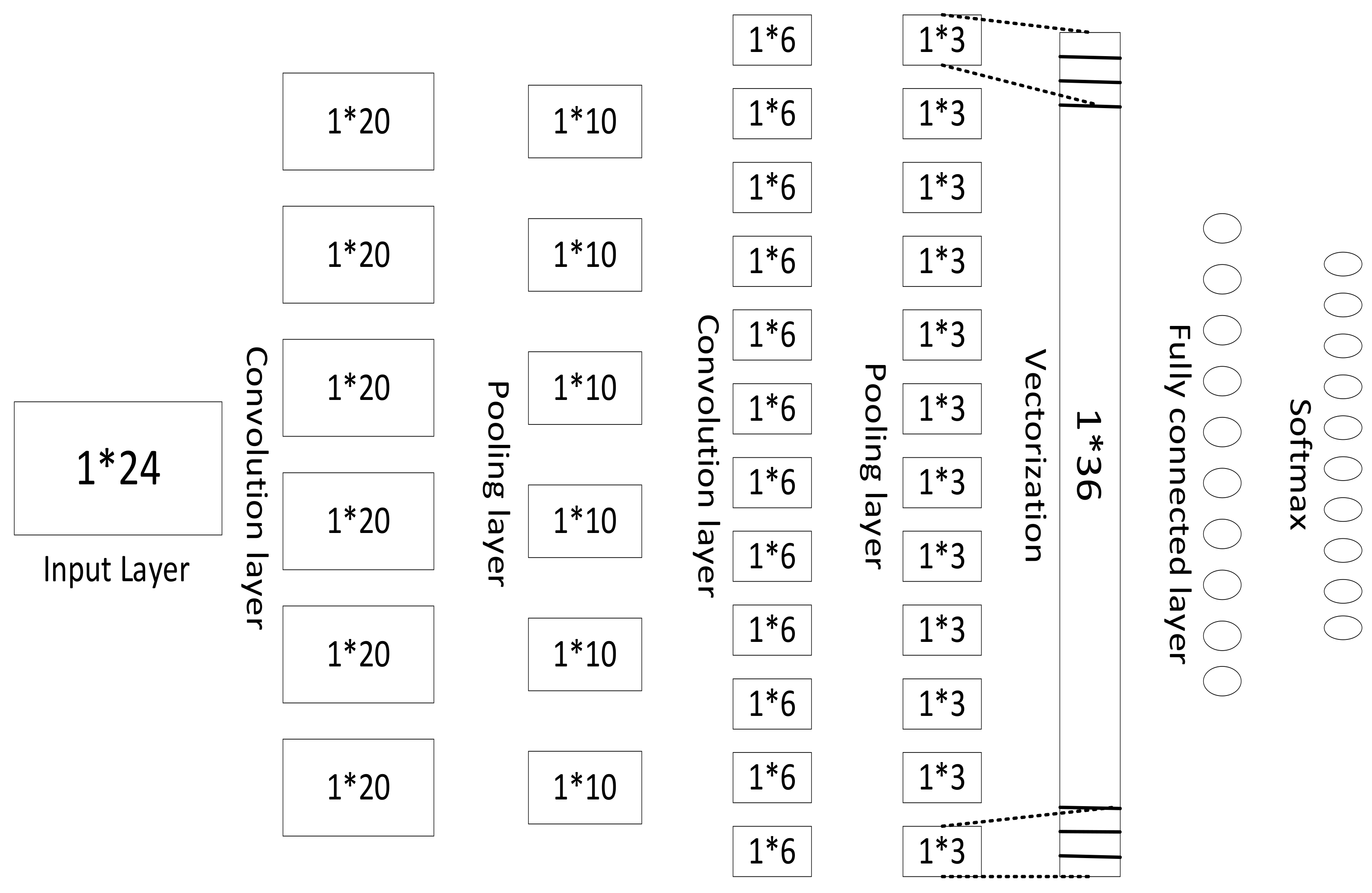
4.2. Experimental Process of One-Dimensional Convolutional Neural Network

Based on the comparison results, CNN is chosen as the method for haze level prediction. Regarding the characteristics of haze, its uneven distribution is not suitable for analysis and research on the changing law of haze. Therefore, in this article, the haze data are divided into subcategories, with 35 micrograms/m³ as a level, so that the data can be fully utilized. The input and training results of different lengths are first analyzed to specify the best training length. The specific parameters of the final selected 24 h sequence for the input length of the one-dimensional convolutional neural network are shown in Figure 5:

From the above figure, we can see the number of convolution kernels and the size of the data after each layer processing. For the unmarked parameters, further description is made here: The size of the convolution kernel taken by the first layer convolution is 1*5, the selected step size is 1, and there is no zero padding. The pooling layer window size is 1*2, which can reduce the feature data to 50%; the second convolution kernel size is still 1*5, the step size is 1, there is no zero padding, and the pooling layer is also 1*2. The haze concentration data for five years were iterated in 2000 rounds, and the network reached the optimal value. The training results are shown in Figure 6.

From the accuracy graph and the loss function graph shown in Figure 6 and Figure 7, we can conclude that the predicted results of this method are over 95%. This shows that the haze concentration level at a certain moment has a nonlinear relationship with the haze concentration of the previous day. Moreover, this nonlinear mapping relationship can be well fitted by the one-dimensional convolutional neural network.

5. Discussion

Based on the one-dimensional haze concentration data from the Machine Learning Repository at Peking University, this paper compared two machine learning methods on their performance on the next prediction based on the past 24 h measurement. The convolutional neural network rises quickly in a short time, but the subsequent changes are not significant. The accuracy rate of the GRU increases with the increase in the number of iterations. It can be said that the GRU neural network is more suitable for tasks with sufficient data volume and no requirement for training time.

The 1D-CNN method shows a higher learning speed and a better performance in general, so it was chosen as the method used for haze concentration prediction in this paper. Through the one-dimensional convolutional neural network proposed in this paper, the haze concentration in the past 24 h can be used to predict the haze concentration level at the next moment.

In the study and prediction of haze, most studies use images or other multidimension data to predict haze in larger areas, which requires a very complex method with a long training time [43,44,45,46]. Compared with other research in the field of haze study and prediction [2,39,47], this paper used single-dimension haze concentration data to predict the near-future haze and achieved a high accuracy, which requires a minimum amount of data to start and a quick learning speed as compared with other learning methods. Though the method could only provide the prediction results for the next time step, the method could be used for prediction into the further future by using the prediction value for the next step prediction. This choice will make the reliability of the second prediction lower than the first, but according to the accuracy of the prediction shown in the Results section, it still presents reliable information for the future.

6. Conclusions

Based on the rising global air pollution issue, this paper aims to produce a simple and accurate method to predict haze levels in the future. This paper chose the data set produced by Peking University to train and test the proposed 1D-CNN to predict the next hour haze concentration based on the known data of the past 24 h and achieved a high accuracy.

Since this study is specific to a research area, there may be insufficient total amounts of haze information in the general area, and the data requirements of large networks cannot be met. However, if it is used in other regions, it is necessary to establish a database by itself, and using a one-dimensional convolutional neural network can alleviate this requirement to some extent. Specifically, the advantages of one-dimensional convolutional neural networks for learning methods of cyclic neural networks fall into two aspects:

• The connection between layers in a convolutional neural network is sparsely connected and convoluted using a convolution kernel that is much smaller than the size of the input data, resulting in a smaller feature vector. This not only reduces the number of parameters but also reduces the storage size of the model, and the requirements for the amount of calculation are greatly reduced. Therefore, the efficiency of the one-dimensional convolutional neural network is significantly improved, and the time complexity is also greatly reduced.
• Parameter sharing: This makes the convolutional neural network robust to the translation of the input data. We can obtain the characteristics of these sequences by a one-dimensional convolution calculation. If we shift this feature event in the input, that is, delay it backward for a period of time, the convolution will still have exactly the same output value, but with the time delayed. This feature is beneficial for the extraction of time-dimensional features by one-dimensional convolutional neural networks and improves the accuracy of the network’s fitting of nonlinear mapping between input and output.

Due to the lack of studies on using haze concentration to predict future concentration, this paper produces a simple yet robust way to fill its absence. However, there are some limits of this method that could be further improved in the future. Since the proposed method is heavily dependent on the precollection and sorting of the data, this method may not be applicable to other locations where the historical data are not sufficient or large enough for this method to be carried out. On the other hand, this method could be combined with other methods, including the haze level converting from AOD and other spatial pattern studies of haze. By combining haze level converted from other data sets, this method could be used for areas without a measure station that have well collected and sorted data. When combined with other spatial pattern studies on haze, this method could support the study by producing reliable data for the unknown future.

References

1. Zhang, Y.; Ma, G.; Yu, F.; Cao, D. Health damage assessment due to PM2. 5 exposure during haze pollution events in Beijing-Tianjin-Hebei region in January 2013. Zhonghua Yi Xue Za Zhi 2013, 93, 2707–2710. [Google Scholar] [PubMed]
2. Zheng, W.; Li, X.; Xie, J.; Yin, L.; Wang, Y. Impact of human activities on haze in Beijing based on grey relational analysis. Rend. Lincei 2015, 26, 187–192. [Google Scholar] [CrossRef]
3. Zheng, W.; Liu, X.; Yin, L. Sentence Representation Method Based on Multi-Layer Semantic Network. Appl. Sci. 2021, 11, 1316. [Google Scholar] [CrossRef]
4. Ma, Z.; Zheng, W.; Chen, X.; Yin, L. Joint embedding VQA model based on dynamic word vector. PeerJ Comput. Sci. 2021, 7, e353. [Google Scholar] [CrossRef] [PubMed]
5. Zheng, W.; Liu, X.; Ni, X.; Yin, L.; Yang, B. Improving Visual Reasoning Through Semantic Representation. IEEE Access 2021, 9, 91476–91486. [Google Scholar] [CrossRef]
6. Zheng, W.; Yin, L.; Chen, X.; Ma, Z.; Liu, S.; Yang, B. Knowledge base graph embedding module design for Visual question answering model. Pattern Recognit. 2021, 120, 108153. [Google Scholar] [CrossRef]
7. Zheng, W.; Liu, X.; Yin, L. Research on image classification method based on improved multi-scale relational network. PeerJ Comput. Sci. 2021, 7, e613. [Google Scholar] [CrossRef]
8. Li, Y.; Zheng, W.; Liu, X.; Mou, Y.; Yin, L.; Yang, B. Research and improvement of feature detection algorithm based on FAST. Rend. Lincei. Sci. Fis. E Nat. 2021. [Google Scholar] [CrossRef]
9. Li, X.; Yin, L.; Yao, L.; Yu, W.; She, X.; Wei, W. Seismic spatiotemporal characteristics in the Alpide Himalayan Seismic Belt. Earth Sci. Inform. 2020, 13, 883–892. [Google Scholar] [CrossRef]
10. Tang, Y.; Liu, S.; Li, X.; Fan, Y.; Deng, Y.; Liu, Y.; Yin, L. Earthquakes spatio–temporal distribution and fractal analysis in the Eurasian seismic belt. Rend. Lincei Sci. Fis. E Nat. 2020, 31, 203–209. [Google Scholar] [CrossRef]
11. Yin, L.; Li, X.; Zheng, W.; Yin, Z.; Song, L.; Ge, L.; Zeng, Q. Fractal dimension analysis for seismicity spatial and temporal distribution in the circum-Pacific seismic belt. J. Earth Syst. Sci. 2019, 128, 22. [Google Scholar] [CrossRef] [Green Version]
12. Zheng, W.; Li, X.; Yin, L.; Yin, Z.; Yang, B.; Liu, S.; Song, L.; Zhou, Y.; Li, Y. Wavelet analysis of the temporal-spatial distribution in the Eurasia seismic belt. Int. J. Wavelets Multiresolut. Inf. Process. 2017, 15, 1750018. [Google Scholar] [CrossRef]
13. Li, X.; Zheng, W.; Wang, D.; Yin, L.; Wang, Y. Predicting seismicity trend in southwest of China based on wavelet analysis. Int. J. Wavelets Multiresolut. Inf. Process. 2015, 13, 1550011. [Google Scholar] [CrossRef]
14. Li, X.; Zheng, W.; Lam, N.; Wang, D.; Yin, L.; Yin, Z. Impact of land use on urban water-logging disaster: A case study of Beijing and New York cities. Environ. Eng. Manag. J. 2017, 16, 1211–1216. [Google Scholar]
15. Holben, B.N.; Eck, T.F.; Slutsker, I.A.; Tanre, D.; Buis, J.; Setzer, A.; Vermote, E.; Reagan, J.A.; Kaufman, Y.; Nakajima, T. AERONET—A federated instrument network and data archive for aerosol characterization. Remote Sens. Environ. 1998, 66, 1–16. [Google Scholar] [CrossRef]
16. Pérez, P.; Trier, A.; Reyes, J. Prediction of PM2.5 concentrations several hours in advance using neural networks in Santiago, Chile. Atmos. Environ. 2000, 34, 1189–1196. [Google Scholar] [CrossRef]
17. Grivas, G.; Chaloulakou, A. Artificial neural network models for prediction of PM10 hourly concentrations, in the Greater Area of Athens, Greece. Atmos. Environ. 2006, 40, 1216–1229. [Google Scholar] [CrossRef]
18. Marzano, F.S.; Rivolta, G.; Coppola, E.; Tomassetti, B.; Verdecchia, M. Rainfall nowcasting from multisatellite passive-sensor images using a recurrent neural network. IEEE Trans. Geosci. Remote Sens. 2007, 45, 3800–3812. [Google Scholar] [CrossRef]
19. Slini, T.; Kaprara, A.; Karatzas, K.; Moussiopoulos, N. PM10 forecasting for Thessaloniki, Greece. Environ. Model. Softw. 2006, 21, 559–565. [Google Scholar] [CrossRef]
20. Zheng, W.; Li, X.; Yin, L.; Wang, Y. The retrieved urban LST in Beijing based on TM, HJ-1B and MODIS. Arab. J. Sci. Eng. 2016, 41, 2325–2332. [Google Scholar] [CrossRef]
21. Chen, X.; Yin, L.; Fan, Y.; Song, L.; Ji, T.; Liu, Y.; Tian, J.; Zheng, W. Temporal evolution characteristics of PM2.5 concentration based on continuous wavelet transform. Sci. Total Environ. 2020, 699, 134244. [Google Scholar] [CrossRef]
22. Li, X.; Zheng, W.; Yin, L.; Yin, Z.; Song, L.; Tian, X. Influence of social-economic activities on air pollutants in Beijing, China. Open Geosci. 2017, 9, 314–321. [Google Scholar] [CrossRef] [Green Version]
23. Zheng, W.; Li, X.; Yin, L.; Wang, Y. Spatiotemporal heterogeneity of urban air pollution in China based on spatial analysis. Rend. Lincei 2016, 27, 351–356. [Google Scholar] [CrossRef]
24. Sun, Y.; Zhuang, G.; Tang, A.; Wang, Y.; An, Z. Chemical characteristics of PM2.5 and PM10 in haze−fog episodes in Beijing. Environ. Sci. Technol. 2006, 40, 3148–3155. [Google Scholar] [CrossRef]
25. Yin, Z.; Wang, H. Seasonal prediction of winter haze days in the north central North China Plain. Atmos. Chem. Phys. 2016, 16, 14843–14852. [Google Scholar] [CrossRef] [Green Version]
26. Xingjian, S.; Chen, Z.; Wang, H.; Yeung, D.-Y.; Wong, W.-K.; Woo, W.-C. Convolutional LSTM network: A Machine Learning Approach for Precipitation Nowcasting. Available online: https://papers.nips.cc/paper/2015/hash/07563a3fe3bbe7e3ba84431ad9d055af-Abstract.html (accessed on 1 September 2021).
27. Klein, B.; Wolf, L.; Afek, Y. A dynamic convolutional layer for short range weather prediction. In Proceedings of the IEEE Conference on Computer Vision and Pattern Recognition, Boston, MA, USA, 7–12 June 2015; pp. 4840–4848. [Google Scholar]
28. LeCun, Y.; Bengio, Y. Convolutional networks for images, speech, and time series. Handb. Brain Theory Neural Netw. 1995, 3361, 1995. [Google Scholar]
29. Schroff, F.; Kalenichenko, D.; Philbin, J. Facenet: A unified embedding for face recognition and clustering. In Proceedings of the IEEE Conference on Computer Vision and Pattern Recognition, Boston, MA, USA, 7–12 June 2015; pp. 815–823. [Google Scholar]
30. Xu, C.; Yang, B.; Guo, F.; Zheng, W.; Poignet, P. Sparse-view CBCT reconstruction via weighted Schatten p-norm minimization. Optics Express 2020, 28, 35469–35482. [Google Scholar] [CrossRef]
31. Liu, S.; Wang, L.; Liu, H.; Su, H.; Li, X.; Zheng, W. Deriving bathymetry from optical images with a localized neural network algorithm. IEEE Trans. Geosci. Remote Sens. 2018, 56, 5334–5342. [Google Scholar] [CrossRef]
32. Ding, Y.; Tian, X.; Yin, L.; Chen, X.; Liu, S.; Yang, B.; Zheng, W. Multi-Scale Relation Network for Few-Shot Learning Based on Meta-Learning; Springer: Cham, Switzerland, 2019; pp. 343–352. [Google Scholar]
33. Ni, X.; Yin, L.; Chen, X.; Liu, S.; Yang, B.; Zheng, W. Semantic representation for visual reasoning. In Proceedings of the MATEC Web of Conferences, Les Ulis, France, 2 June 2019. [Google Scholar]
34. Tang, Y.; Liu, S.; Deng, Y.; Zhang, Y.; Yin, L.; Zheng, W. An improved method for soft tissue modeling. Biomed. Signal Process. Control. 2021, 65, 102367. [Google Scholar] [CrossRef]
35. Tang, Y.; Liu, S.; Deng, Y.; Zhang, Y.; Yin, L.; Zheng, W. Construction of force haptic reappearance system based on Geomagic Touch haptic device. Comput. Methods Programs Biomed. 2020, 190, 105344. [Google Scholar] [CrossRef]
36. Yang, B.; Liu, C.; Huang, K.; Zheng, W. A triangular radial cubic spline deformation model for efficient 3D beating heart tracking. Signal Image Video Process. 2017, 11, 1329–1336. [Google Scholar] [CrossRef] [Green Version]
37. Krizhevsky, A.; Sutskever, I.; Hinton, G.E. Imagenet classification with deep convolutional neural networks. Adv. Neural Inf. Process. Syst. 2012, 25, 1097–1105. [Google Scholar] [CrossRef]
38. Szegedy, C.; Liu, W.; Jia, Y.; Sermanet, P.; Reed, S.; Anguelov, D.; Erhan, D.; Vanhoucke, V.; Rabinovich, A. Going deeper with convolutions. In Proceedings of the IEEE Conference on Computer Vision and Pattern Recognition, Boston, MA, USA, 7–12 June 2015; pp. 1–9. [Google Scholar]
39. Zhang, J.; Min, X.; Zhu, Y.; Zhai, G.; Zhou, J.; Yang, X.; Zhang, W. HazDesNet: An End-to-End Network for Haze Density Prediction. IEEE Trans. Intell. Transp. Syst. 2020, 1–16. [Google Scholar] [CrossRef]
40. Tran, T.N.; Phuc, D.T. Grid search of multilayer perceptron based on the walk-forward validation methodology. Int. J. Electr. Comput. Eng. 2021, 11, 1742. [Google Scholar]
41. Żbikowski, K. Using volume weighted support vector machines with walk forward testing and feature selection for the purpose of creating stock trading strategy. Expert Syst. Appl. 2015, 42, 1797–1805. [Google Scholar] [CrossRef]
42. Dey, R.; Salem, F.M. Gate-variants of gated recurrent unit (GRU) neural networks. In Proceedings of the 2017 IEEE 60th International Midwest Symposium on Circuits and Systems (MWSCAS), Boston, MA, USA, 6–9 August 2017; pp. 1597–1600. [Google Scholar]
43. Bahari, R.; Abbaspour, R.A.; Pahlavani, P. Prediction of PM2.5 concentrations using temperature inversion effects based on an artificial neural network. In Proceedings of the ISPRS International Conference of Geospatial Information Research, Tehran, Iran, 15–17 November 2014; p. 17. [Google Scholar]
44. Mogireddy, K.; Devabhaktuni, V.; Kumar, A.; Aggarwal, P.; Bhattacharya, P. A new approach to simulate characterization of particulate matter employing support vector machines. J. Hazard. Mater. 2011, 186, 1254–1262. [Google Scholar] [CrossRef]
45. Hooyberghs, J.; Mensink, C.; Dumont, G.; Fierens, F.; Brasseur, O. A neural network forecast for daily average PM10 concentrations in Belgium. Atmos. Environ. 2005, 39, 3279–3289. [Google Scholar] [CrossRef]
46. Voukantsis, D.; Karatzas, K.; Kukkonen, J.; Räsänen, T.; Karppinen, A.; Kolehmainen, M. Intercomparison of air quality data using principal component analysis, and forecasting of PM10 and PM2.5 concentrations using artificial neural networks, in Thessaloniki and Helsinki. Sci. Total Environ. 2011, 409, 1266–1276. [Google Scholar] [CrossRef] [PubMed]
47. Yeh, C.-H.; Huang, C.-H.; Kang, L.-W. Multi-scale deep residual learning-based single image haze removal via image decomposition. IEEE Trans. Image Process. 2019, 29, 3153–3167. [Google Scholar] [CrossRef] [PubMed]
Figure 1. General structure of one-dimensional convolutional neural networks. From left to right: input layer; convolution layer; pooling layer; connection layer; and classification layer.
Atmosphere 12 01327 g001
Figure 2. Sparse connection diagram of one-dimensional convolution.
Atmosphere 12 01327 g002
Figure 3. Accuracy of one-dimensional convolutional neural network.
Atmosphere 12 01327 g003
Figure 4. GRU circular neural network accuracy diagram.
Atmosphere 12 01327 g004
Figure 5. One-dimensional convolutional neural network predicts the specific structure of haze. From left to right: input layer; convolution layer; pooling layer; convolution layer; pooling layer; vectorization layer; connection layer; classification.
Atmosphere 12 01327 g005
Figure 6. Prediction accuracy diagram of haze classification by 1D-convolutional neural network.
Atmosphere 12 01327 g006
Figure 7. Loss function in training of 1D-convolutional neural network.
Atmosphere 12 01327 g007