Article

Crop Residue Burning in Northeast China and Its Impact on PM2.5 Concentrations in South Korea

1
Air Quality Forecasting Center, National Institute of Environmental Research, Incheon 22689, Korea
2
National Air Emission Inventory and Research Center, Chungju-si 28166, Korea
3
Air Quality Research Division, National Institute of Environmental Research, Incheon 22689, Korea
4
Division of Forest Science, Kangwon National University, Chuncheon-si 24341, Korea
*
Authors to whom correspondence should be addressed.
Atmosphere 2021, 12(9), 1212; https://doi.org/10.3390/atmos12091212
Submission received: 19 August 2021 / Revised: 7 September 2021 / Accepted: 13 September 2021 / Published: 16 September 2021
(This article belongs to the Section Aerosols)

Abstract

:
The impact of crop residue burning in northeastern China on South Korean PM2.5 concentrations was assessed via weather conditions, air quality modeling (AQM), and PM2.5 composition data during two cases exceeding 35 µg·m−3 in November 2015. PM2.5 concentration simulations of Case 1 differed from observations by 3.7–17.6 µg·m−3, overestimating the levels by 6–36%; however, Case 2 varied by 20.0–59.8 µg·m−3 from observations, with a 53–91% underestimation. Case 1 was generally well simulated, whereas the Case 2 simulation failed because the emissions of crop residue burning in northeastern China, as confirmed through satellite analysis (MODIS fires and thermal anomalies) and previous research, were not considered. The portion of organic/elemental carbon ratio during Case 2 was 1.6–2.3 times higher than that of Case 1. These results suggest that it is necessary to consider the effects of crop residue burning in northeast China to establish countermeasures to improve air quality and air quality forecasting in South Korea.

1. Introduction

PM2.5 is particulate matter with an aerodynamic diameter < 2.5 μm that can harmfully affect human health by causing cardiovascular and respiratory diseases and cancer, as well as increasing early mortality [1,2,3,4,5]. The Organization for Economic Cooperation and Development (OECD) projected that the early deaths from outdoor air pollution in 2060 will triple those in 2010, and the resulting losses of gross domestic product (GDP) will be 2.6% for China and 0.6% for South Korea, representing the two most drastically impacted nations among OECD members [6]. Accordingly, to adequately address this issue, the causes of PM2.5 must be understood, and appropriate measures must be undertaken.
Among the sources of PM2.5, which can be classified into natural emissions such as forest fires or yellow dust and anthropogenic emissions that originate from factories or cars, the gaseous and particulate pollutants produced by human activities are the largest contributors [7,8,9]. In particular, South Korean PM2.5 concentrations are dependent on domestic pollutants and the influx of foreign pollutants via long-range transport [10]. Located within the westerly wind zone, pollutants produced on the windward side can be transported into South Korea [11,12,13,14]. Particulate levels also vary with meteorological conditions. If high atmospheric pressure forms without precipitation, the wind speed will be extremely weak to diffuse pollutants, thereby increasing PM2.5 concentrations; however, in high wind speeds, significant diffusion takes place, decreasing the pollutant levels [15,16]. In particular, it is expected that the long-range transport of foreign pollutants creating high PM2.5 concentrations in South Korea will increase in the future [17,18,19,20]. It has also been found that pollutants produced from the northeastern region of China, located in the windward position of South Korea, can directly influence the air quality of South Korea [21,22].
The industrial and economic sectors of northeastern China are based on traditional industries such as crop cultivation, and 30% of the land area is dedicated to agriculture [23]. The burning of surplus crops has continuously occurred throughout this non-growing agricultural season in northeastern China. Furthermore, although this area reportedly possesses a larger amount of crop residues burned on site compared to other regions of China [24,25,26,27], the research surrounding the correlated impacts on PM2.5 concentrations in South Korea is insufficient. Therefore, the impact of crop burning in northeastern China on the PM2.5 concentration in South Korea was investigated in this study by analyzing meteorological data, air quality simulations, PM2.5 concentrations, and composition data during the high-concentration periods of November 2015.

2. Materials and Methods

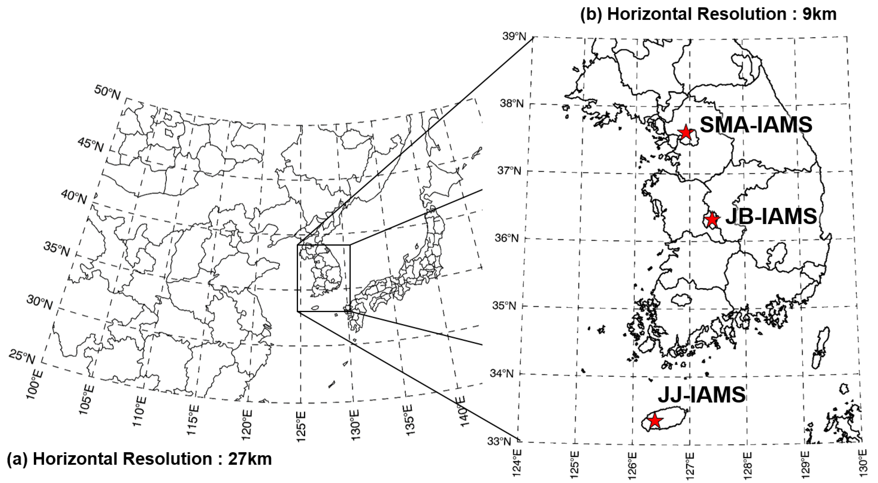
2.1. Ground and Satellite Data

Among the monitoring networks operated by the Ministry of Environment of South Korea, this study utilized the data collected from 2 November to 12 November, 2015, by Intensive Air Pollution Monitoring Stations in Seoul (SMA-IAMS), Daejeon (JB-IAMS), and Jeju (JJ-IAMS), which recorded PM2.5 mass, organic carbon (OC) and elemental carbon (EC) compositions, and ion composition (SO42− and NO3; Figure 1b). SMA-IAMS is located in an urban center with densely packed buildings, JB-IAMS is located in a residential and commercial district in the vicinity of a six-lane road, and JJ-IAMS is 600 m above sea level on the west side of Mt. Hallasan to monitor the national background PM concentrations and long-range pollutant transport [28].
To investigate pollutant source and transport trajectory, moderate-resolution imaging spectrometer (MODIS) fires and thermal anomalies data (https://worldview.earth-data.nasa.gov, accessed on 6 April 2021), and the hybrid single-particle Lagrangian trajectory (HYSPLIT) of the National Oceanic and Atmospheric Administration/Air Resources Laboratory (NOAA/ARL) were utilized [29]. The MODIS data maintained a daily 1 km × 1 km resolution, employing Terra (MOD14) and Aqua (MYD14) satellite data [30] to detect thermal sources, such as fires, from 4 November to 8 November, 2015. HYSPLIT analyzed the rear trajectory for the centrally located JB-IAMS site at 100, 200, and 500 m on 2 November (21:00 KST) and 10 November (03:00 KST).

2.2. Air Quality Model

To analyze the meteorological conditions and air quality changes in northeastern Asia, the Weather Research and Forecast (WRF) v.3.3 meteorological model [31], Sparse Matrix Operator Kernel Emission (SMOKE) v.3.1 emission processing model [32], and Community Modeling Air Quality (CMAQ) v.4.7.1 air quality model [33] were used. The emission inventory for the air quality simulation used the Model Inter Comparison Study for Asia (MICS-Asia) 2010 [34] for foreign regions and the Clean Air Policy Support System (CAPSS) 2010 emission list for domestic regions. For the initial and boundary conditions of the WRF, the simulated results of the unified model (UM) provided by the Korea Meteorological Administration (KMA) were used. The WRF meteorological simulation was used as the input data for the air quality model of the Meteorology Chemistry Interface Processor (MCIP) v.3.6 (Figure 1a) [35].
The air quality modeling (AQM) area was a nested grid consisting of domain 1, including northeastern Asia, and domain 2, comprising only the Korean Peninsula (Figure 1b). Domain 1 was 128 × 174 grids along the latitude and longitude, respectively, with a 27 km horizontal grid resolution; domain 2 was 82 × 67 grids along the latitude and longitude, respectively, with a 9 km horizontal grid resolution. The two domains were constructed equally in the vertical direction to simulate air quality up to 19 km above ground level, and the stretching grid of the lower section was used to generate 15 layers for vertical grid decomposition.
The major components of the meteorological and air quality models are listed in Table 1. The Yonsei University Scheme (YUS) [36] was used as the planetary boundary layer for the WRF model. For cloud microphysics, the WRF Single Moment 3 Class (WSM3) [37,38] was used, and the Kain-Fritsch scheme [39] was selected for the cumulus cloud option. The fifth-generation CMAQ aerosol module (AERO5) was selected for the air quality model (AQM) [40]. For the chemical mechanism, the Statewide Air Pollution Research Center v.99 (SAPRC 99) [41] was used, and for the horizontal diffusion, the YAMO scheme was used [42].

3. Results and Discussion

There were two instances where the PM2.5 exceeded 35 µg·m−3 at each of the three IAMSs, which corresponded to an “Unhealthy” rating according to the Korean forecast system. The first (Case 1) was from 2 November (15:00 KST) to 6 November (14:00 KST) for SMA-IAMS, and the second (Case 2) was from 10 November (01:00 KST) to 11 November (10:00 KST). At JB-IAMS, the cases were observed from 2 November (17:00 KST) to 6 November (11:00 KST) and from 10 November (02:00 KST) to 11 November (13:00 KST); at JJ-IAMS, the cases were observed from 2 November (19:00 KST) to 3 November (10:00 KST) and 9 November (11:00 KST) to 11 November (09:00 KST).

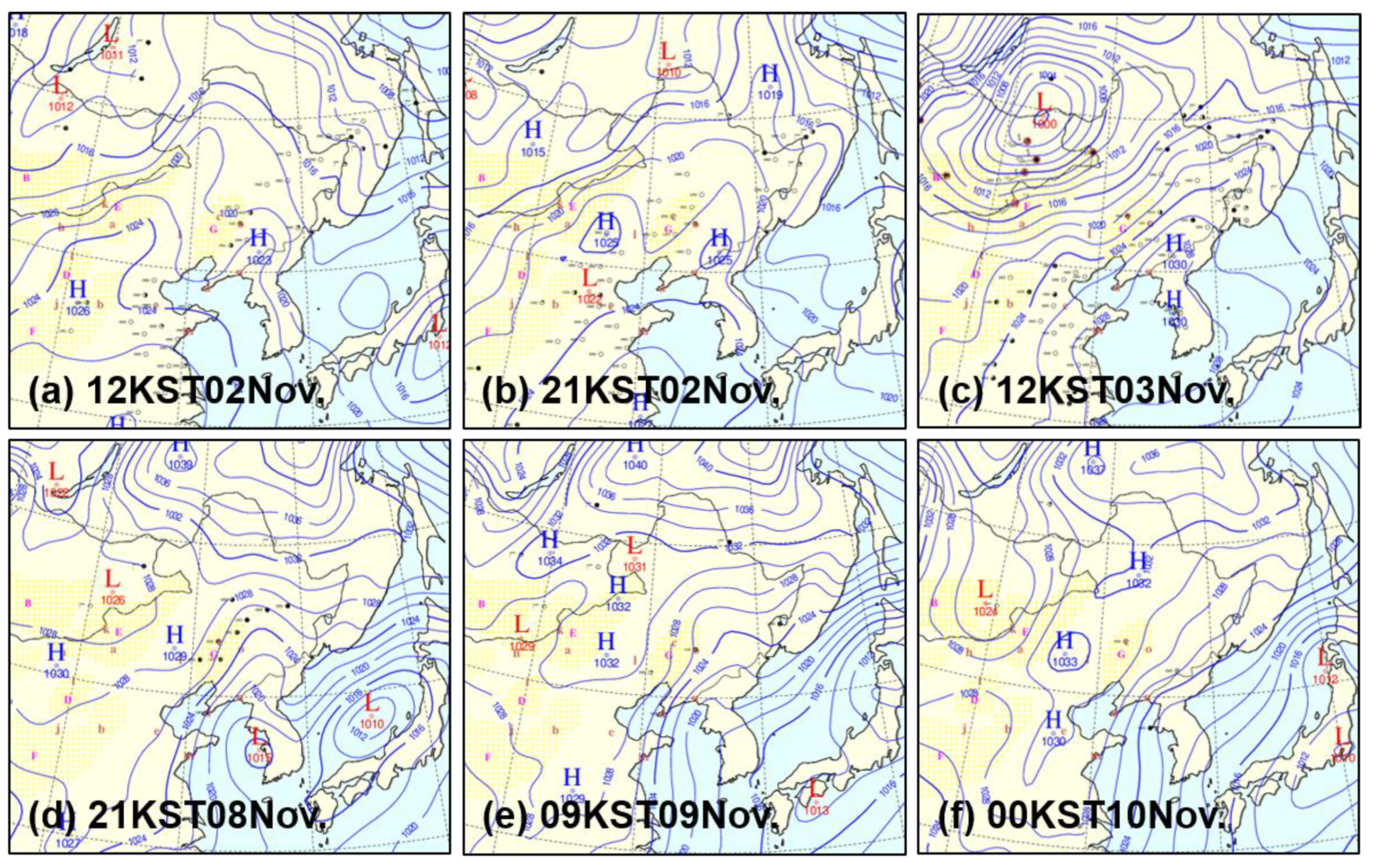
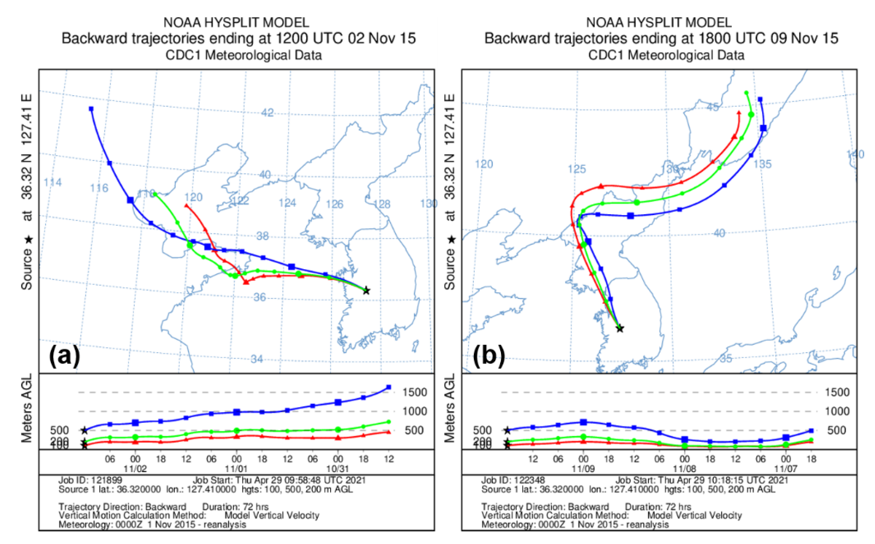
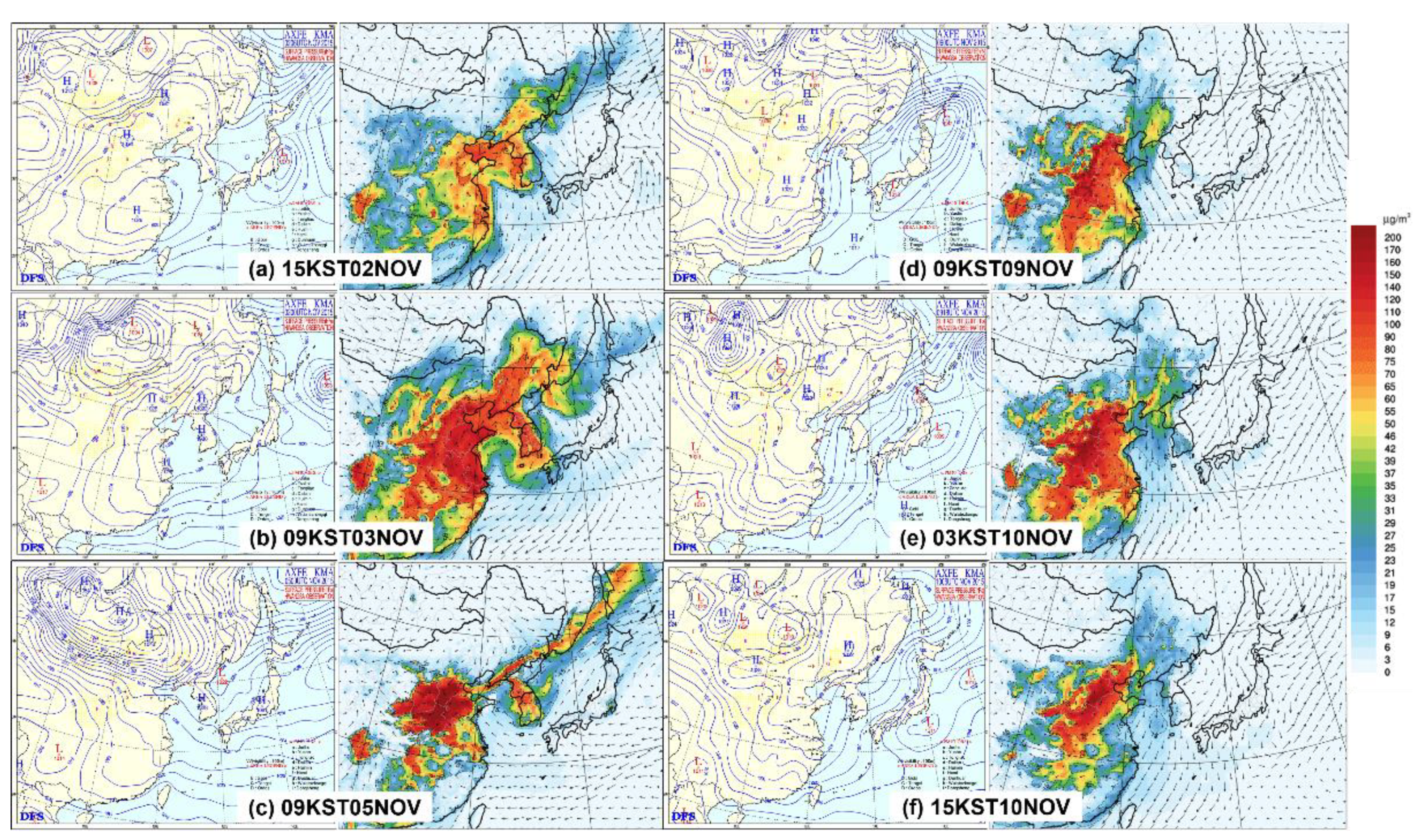
3.1. Meteorological Conditions
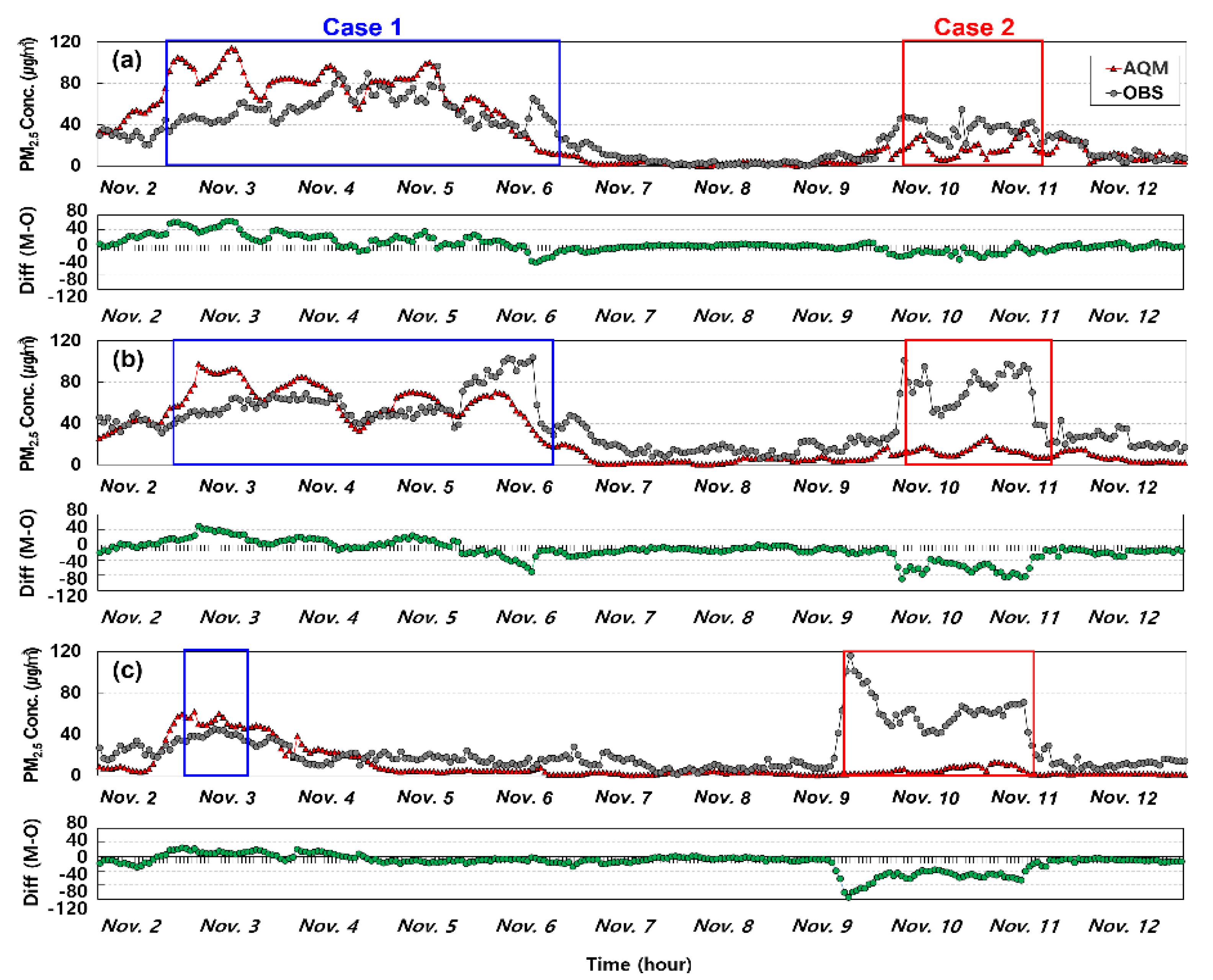
To assess the meteorological conditions of Case 1 and 2, the yellow dust weather list provided by the KMA was used. Figure 2 illustrates the early stages of the high PM concentrations in each case. For Case 1, a high-pressure system was formed in central China, forming favorable conditions for westerly or northwesterly airflow to South Korea along with the high-pressure air circulation (clockwise; Figure 2a). From the afternoon of 2 November, this high-pressure system slowly migrated and settled in South Korea (Figure 2b) on 3 November (Figure 2c). Owing to this movement, the westerly to northwesterly air current was formed on the afternoon of 2 November, and by 3 November, the air was relatively stagnant due to the influence of the South Korean high-pressure system. During Case 2, South Korea was affected by a low-pressure system on 8 November (Figure 2d), and on 9 November, then it was replaced by a high-pressure system as it moved toward Japan (Figure 2e). Thus, the westside of South Korea was under a high-pressure system, whereas the eastside experienced low-pressure conditions, leading to the formation of a north wind/air current. On 10 November, the same air pressure placement persisted, although the gradient had increased; thus, the north wind/air current remained, providing the meteorological conditions for stronger wind formation on 10 November (Figure 2f).
To study the initial air patterns during the high PM concentration events, a rear trajectory analysis was performed based on the centrally located JB-IAMS data. Figure 3a shows these back-projected results for 2 November at 21:00 KST and suggests that South Korea was affected by the air current around Shantung Province. The northwesterly air changed to a westerly–northwesterly flow by 31 October 09:00 KST, becoming uniformly westerly as of 1 November 09:00 KST. Figure 3b shows these results for 10 November 03:00 KST and suggests that South Korea was affected by an air current from the wind-ward region. On 7 November 09:00 KST, the air current flowing via the northerly winds from Russia was affected by the easterly winds, moving to the boundary of northeastern China and North Korea. Then, by 8 November 09:00 KST, it was affected by the northerly winds, moving into South Korea.
During the initial stages of high PM concentrations, the pressure placement and air pattern analyses suggested that South Korea was subjected to a (north) westerly airflow in Case 1 and a northerly airflow in Case 2. Their specific roles in creating the high PM concentrations observed in South Korea are described in Section 3.2, Section 3.3 and Section 3.4.

3.2. AQM

The PM2.5 concentrations were simulated via AQM over the research period. For the SMA-IAMS and JB-IAMS sites, the simulated concentrations of the lowest layer (z = 32 m) were used; however, for JJ-IAMS, located 600 m above sea level, the AQM concentrations at 640 m were used.
Figure 4 illustrates the spatial distribution of the simulated PM2.5 concentrations with weather charts from KMA for Case 1 and Case 2. The simulated wind fields are consistent with the atmospheric pressure patterns shown in weather chart. As detailed in Section 3.1, Case 1 was simulated such that the formation of the west-to-northwesterly airflow contributed to the high PM2.5 concentrations observed. The particulate matter started to get transported to South Korea on 2 November at 15:00 KST (Figure 4a) and lasted for approximately three days (until 5 November) due to foreign transport and stagnant air (Figure 4b,c). The simulated high PM2.5 concentrations began to dissipate on 6 November under the influence of a northerly airflow. For Case 2, a clear north airflow was formed, preventing the high concentrations from being adequately simulated (Figure 4d–f).
The simulated and observed PM2.5 concentrations at SMA-IAMS, JB-IAMS, and JJ-IAMS, as well as their differences, are shown in Figure 5 and Table 2. In Case 1, the AQM overestimated PM2.5 concentrations for all monitoring stations; however, Case 2 was underestimated at each station (Table 2). The average differences between the observed and simulated concentrations were 17.6 µg·m−3, 3.7 µg·m−3, and 14.3 µg·m−3 at SMA-IAMS, JB-IAMS, and JJ-IAMS in Case 1, respectively; however, these locations were underestimated by −20.0 µg·m−3, −59.8 µg·m−3, and −57.6 µg·m−3 in Case 2, respectively. These levels correspond to an overestimation of 31%, 6%, and 36% for Case 1 at SM- JB-, and JJ-IAMS, respectively; however, concentrations were underestimated by 53%, 81%, and 91% in Case 2, respectively.
The overestimation of Case 1 primarily occurred during the early stages of foreign transport; thus, it can be verified that the foreign influx of PM was higher than that observed, likely as a result of the emission list being based on 2010 data and failing to reflect the true situation of 2015.
The underestimation of high concentrations in Case 2 was likely based on nearby crop residue burning (see Section 3.3 and Section 3.4). The foreign emission data, MICS-Asia 2010, used for the air quality simulation in this study classified emission sources as either development, engineering, traffic, residence, or agriculture. For agriculture, only NH3 is included, and crop residue burning and dust scattering are excluded from the emission calculations [34]; therefore, it was found that the high PM2.5 concentrations could not be adequately modeled as foreign emissions from crop burning.

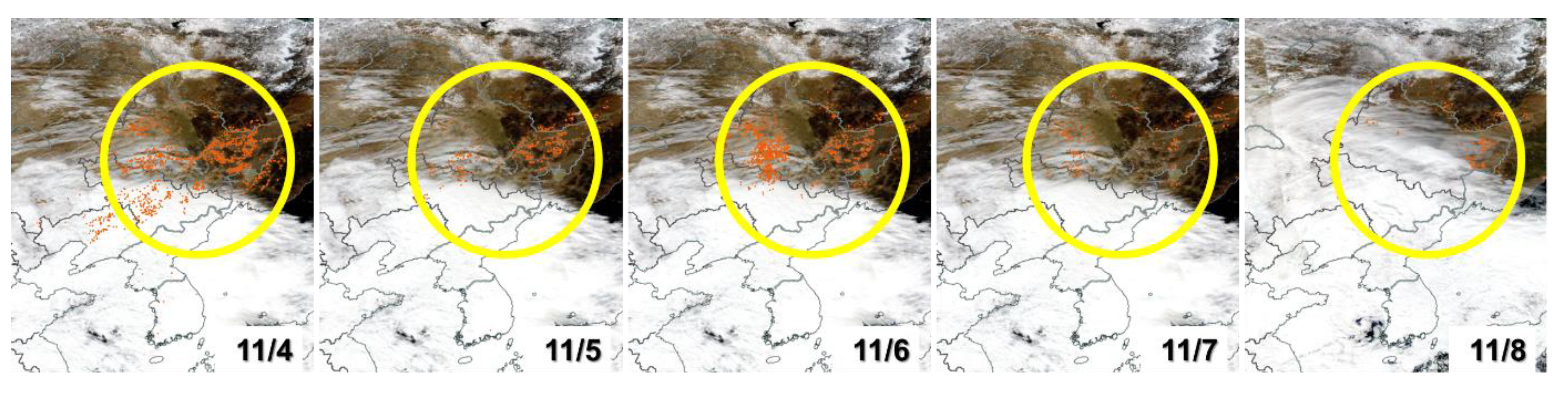
3.3. Crop Residue Burning in Northeastern China

To determine the driving factors behind the failure to model the high-pressure system observed in Case 2, the atmospheric situation of northeastern China, windward of South Korea, was further examined using MODIS fire and thermal anomaly data. The MODIS products from 4 November to 8 November indicated that relatively extensive heat was produced in northeastern China prior to Case 2 (although cloud cover prevented further detection on 7–8 November; Figure 6). According to the PM2.5 network (http://www.pm2.5.in, accessed on 8 November 2015) information on China’s air quality monitoring network, Changchun City in northeastern China, located between Shenyang and Harbin, exhibited a daily PM2.5 average concentration of 536 µg·m−3 on 8 November, a 21-fold increase over the recommended WHO standards of 25 µg·m−3 [46]. On 9 November 00:00, the recorded PM2.5 concentration was 991 µg·m−3, signaling a severe air pollution event; therefore, it was concluded that the heat production and resulting pollution continued to 7–8 November.
Previous research has found that the heat production during Case 2 was due to crop burning. Yin et al. used MODIS data to identify crop residue burning sites in northeastern China [47], concluding that from 4 November to 6 November, daily crop residue burning occurred at 2291, 1050, and 1109 individual sites, respectively. In particular, during the agricultural off-season of northeastern China in November 2015, the highest hourly PM2.5 concentrations reported surpassed 1000 µg·m−3. Furthermore, Zhang et al. reported serious air pollution in Shenyang in 8 November 2015, with PM concentrations of 1326 µg·m−3 [48].

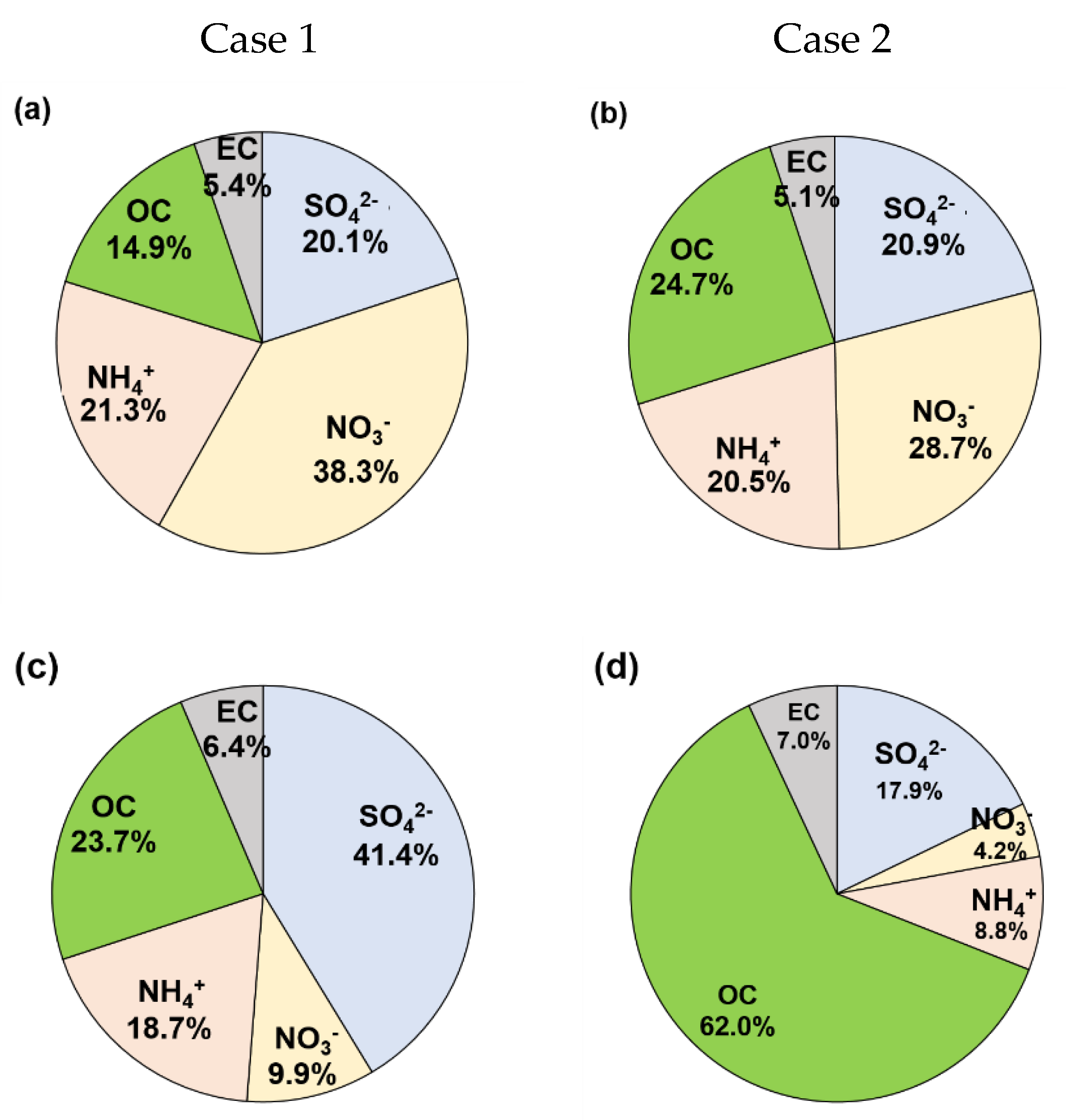
3.4. PM2.5 Composition

The main components of PM2.5 in Cases 1 and 2 are shown in Table 3 and Figure 7. The majority of the composition data are missing from SMA-IAMS owing to the maintenance schedule, and this site was thus removed from this analysis. The observed PM2.5 concentrations at JB-IAMS in Case 1 ranged from 36–104 µg·m−3, with an average of 61.3 µg·m−3 (Table 3). The relative average contribution was highest for NO3 (38.3%), followed by NH4+ (21.3%) and SO42− (20.1%) (Figure 7a). The concentrations of Case 2 ranged from 38–98 µg·m−3 (average of 75.0 µg·m−3) with the highest relative average contributions from NO3 (28.7%), OC (24.7%), and SO42− (20.9%) (Figure 7b). Notably, the relative contribution of NO3 diminished in Case 2, whereas that of OC increased.
The JJ-IAMS site maintained a concentration of 33–45 µg·m−3 in Case 1, with an average of 39.2 µg·m−3 (Table 3). The average component contribution of PM2.5 was highest for SO42− (41.4%), followed by OC (23.7%) and NH4+ (18.7%; Figure 7c). In Case 2, the PM2.5 concentrations ranged from 41–116 µg·m−3 (average 63.4 µg·m−3; Table 3). The relative average contribution was highest for OC (63.6%), followed by SO42− (16.7%) and NH4+ (8.2%; Figure 7d). Accordingly, the relative contribution of SO42− decreased, whereas that of OC significantly increased in Case 2.
For JB-IAMS, NO3 maintained the largest contribution in both cases. To analyze the cause, CAPSS, the emission list data provided by the Ministry of Environment of South Korea, was used to investigate the major domestic emission sources of Junggu, Daejeon, where the site is located [49]. In 2015, the largest PM2.5 emission source was scattered dust and automobile pollution, accounting for 32.8% and 30.9%, respectively (~64% of total emissions). Among automobile pollution sources, NOx accounted for 40% of the pollutants; therefore, it can be inferred that NO3 would have maintained the highest contribution compared to the JJ-IAMS area due to its local characteristics.
Alternatively, the burning of biomass, such as crop residue, primarily emits OC [50], exhibiting a high OC/EC ratio [51,52,53]. As shown in Table 3, this observed ratio at JB-IAMS spanned 1.7–6.2 (average, 3) in Case 1; and in Case 2, this value ranged from 3.3–7.7 (average, 5.0). At JJ-IAMS, the reported range (average) for Case 1 and Case 2 were 3.0–5.4 (3.8) and 6.3–12.4 (8.8), respectively. According to Zhang et al., the OC/EC ratios due to coal burning, car emissions, and biomass burning were 2.7, 1.1, and 9.0, respectively [54]; thus, Case 1 exhibited a ratio more closely corresponding to that of coal burning, and Case 2 more closely resembled levels associated with biomass burning [54].

4. Conclusions

In this study, two cases (Cases 1 and 2) where the PM2.5 concentrations exceeded 35 µg·m−3 during 2–12 November 2015 were analyzed. For Case 2, meteorological conditions, air quality simulations, PM2.5 concentrations, and corresponding composition data were used to study the effects of crop residue burning in northeastern China on the PM2.5 concentrations of South Korea.
As a result of the AQM, the simulated PM2.5 concentrations in Case 1 overestimated the observation values by 3.7–17.6 µg·m−3 (6–36%); however, in Case 2, the simulated values were underestimated by 20.0–59.8 µg·m−3 (53–91%). Despite this overestimation, Case 1 properly simulated the high-concentration phenomena that occurred in South Korea over this period; however, in Case 2, the high concentrations could not be simulated due to a spike in crop residue burning that occurred over this time. Based on the satellite data and preceding research, it was confirmed that there were crop residue burning events in the northeastern regions of China throughout this period, and when compared with Case 1, Case 2 had significantly higher contributions of OC, with an average OC/EC ratio of 8.8 (a 1.6–2.3-fold increase; extremely similar to the expected crop residue burning yields of 9.0). It was confirmed that crop residue burning from the northeastern region of China during the non-growing agricultural off-season significantly affected the air quality of South Korea. However, this study has a limitation that AQM modeling could not be directly performed using the emissions of crop residue burning in northeast China in Case 2, because it was not possible to obtain the available emission information (location, field size, fuel load, etc.) for estimating them.
These results can be used as scientific evidence to plan the policies that need to be enacted in the future to improve South Korean air quality. Particularly, the policies that are going to be enacted in the future aimed at improving South Korean air quality should consider crop residue burning in northeast China. Furthermore, this research has highlighted that the air quality forecasting system may fail to predict high concentrations due to a lack of input data regarding foreign crop residue burning; however, as it is difficult to anticipate crop residue burning in advance due to its irregular periodicity, it is suggested here that the performance of any AQM must be improved via the inclusion of air quality data assimilation of satellite and ground data.

Author Contributions

Supervision, J.-B.L. and S.-D.L.; Writing—original draft, J.-J.L.; Writing—review & editing, J.-B.L. and S.-D.L.; Investigation, G.H.; Data curation, O.K. and H.L.; Formal analysis, D.L. and D.-g.K.; Visualization, J.-J.L. All authors have read and agreed to the published version of the manuscript.

Funding

This research was funded by the National Institute of Environmental Research and funded by the Ministry of Environment (NIER-2021-01-01-086), supported by Basic Science Research Program through the National Research Foundation of Korea (NRF) funded by the Ministry of Education (NRF-2021R1F1A1062524), and supported by 2018 Research Grant from Kangwon National University.

Institutional Review Board Statement

Not applicable.

Informed Consent Statement

Not applicable.

Data Availability Statement

Data set available on request to corresponding authors.

Conflicts of Interest

The authors declare no conflict of interest.

References

  1. Feng, S.; Gao, D.; Liao, F.; Zhou, F.; Wang, X. The health effects of ambient PM2.5 and potential mechanisms. Ecotoxicol. Environ. Saf. 2016, 128, 67–74. [Google Scholar] [CrossRef] [PubMed]
  2. International Agency for Research on Cancer (IARC). Outdoor Air Pollution. 2015. Available online: https://publications.iarc.fr/Book-And-Report-Series/Iarc-Monographs-On-The-Identification-Of-Carcinogenic-Hazards-To-Humans/Outdoor-Air-Pollution-2015 (accessed on 3 May 2021).
  3. Nishiwaki, Y.; Michikawa, T.; Takebayashi, T.; Nitta, H.; Iso, H.; Inoue, M.; Tsugane, S. Long-term exposure to particulate matter in relation to mortality and incidence of cardiovascular disease: The JPHC Study. J. Atheroscler. Thromb. 2013, 20, 296–309. [Google Scholar] [CrossRef] [Green Version]
  4. World Health Organization (WHO). Health Effects of Particulate Matter. 2013. Available online: http://www.euro.who.int/en/health-topics/environment-and-health/air-quality/publications/2013/health-effects-of-particulate-matter.-policy-implications-for-countries-in-eastern-europe,-caucasus-and-central-asia-2013 (accessed on 12 July 2019).
  5. Zoran, D.R.; Miljevic, B.; Surawski, N.C.; Morawska, L.; Gong, K.M.; Goh, F.; Yang, I.A. Respiratory health effects of diesel particulate matter. Asian Pac. Soc. Respirol. 2012, 17, 201–212. [Google Scholar]
  6. Organization for Economic Cooperation and Development (OECD). The Economic Consequences of Outdoor Air Pollution. 2016. Available online: https://www.oecd.org/environment/indicators-modelling-outlooks/Policy-Highlights-Economic-consequences-of-outdoor-air-pollution-web.pdf (accessed on 21 September 2020).
  7. Choi, R.-H.; Kang, W.-S.; Son, C.-S. Particulate matter (PM2.5) state inference by rule induction. J. Embed. Syst. Appl. 2018, 13, 179–185. (In Korea) [Google Scholar] [CrossRef]
  8. Seo, Y.-H. Source profile of PM10 emitted upon agricultural biomass combustion. J. Korea Soc. Environ. Adm. 2014, 20, 1–7, (In Korean with English Abstract). [Google Scholar]
  9. Moon, K.J.; Park, S.M.; Park, J.S.; Song, I.H.; Jang, S.K.; Kim, J.C.; Lee, S.J. Chemical Characteristics and Source Apportionment of PM2.5 in Seoul Metropolitan Area in 2010. J. Korean Soc. Atmos. Environ. 2011, 27, 711–722. (In Korea) [Google Scholar] [CrossRef]
  10. Nam, K.-P.; Lee, D.-G.; Jang, L.-S. Analysis of PM2.5 concentration and contribution characteristics in South Korea according to seasonal weather patterns in East Asia: Focusing on the intensive measurement periods in 2015. Environ. Impact Assess. 2019, 28, 183–200. (In Korea) [Google Scholar] [CrossRef]
  11. Chen, L.; Gao, Y.; Zhang, M.; Fu, J.S.; Zhu, J.; Liao, H.; Li, J.; Huang, K.; Ge, B.; Wang, X.; et al. MICS-Asia III: Multi-model comparison and evaluation of aerosol over East Asia. Atmos. Chem. Phys. 2019, 19, 11911–11937. [Google Scholar] [CrossRef] [Green Version]
  12. Oh, H.-R.; Ho, C.-H.; Kim, J.; Chen, D.; Lee, S.; Choi, Y.-S.; Chang, L.-S.; Song, C.-K. Long-range transport of air pollutants originating in China: A possible major cause of multi-day high-PM10 episodes during cold season in Seoul, Korea. Atmos. Environ. 2015, 109, 23–30. [Google Scholar] [CrossRef]
  13. Ying, Q.; Wu, L.; Zhang, H. Local and inter-regional contributions to PM2.5 nitrate and sulfate in China. Atmos. Environ. 2014, 94, 582–592. [Google Scholar] [CrossRef]
  14. Heo, J.-B.; Hopke, P.K.; Yi, S.-M. Source apportionment of PM2.5 in Seoul, Korea. Atmos. Chem. Phys. 2008, 8, 20427–20461. Available online: http://www.atmos-chem-phys-discuss.net/8/20427/2008/ (accessed on 30 April 2021).
  15. Dawson, J.P.; Adams, P.J.; Pandis, S.N. Sensitivity of PM2.5 to climate in the Eastern US: A modeling case study. Atmos. Chem. Phys. 2007, 7, 4295–4309. Available online: https://www.atmos-chem-phys.net/7/4295/2007/ (accessed on 21 September 2020). [CrossRef] [Green Version]
  16. Tagaris, E.; Manomaiphiboon, K.; Liao, K.-J.; Leung, L.R.; Woo, J.-H.; He, S.; Amar, P.; Russell, A.G. Impacts of global climate change and emissions on regional ozone and fine particulate matter concentrations over the United States. J. Geophys. Res. 2007, 112, D14312. [Google Scholar] [CrossRef]
  17. Lee, D.; Choi, J.-Y.; Myoung, J.; Kim, O.; Park, J.; Shin, H.-J.; Ban, S.-J.; Park, H.-J.; Nam, K.-P. Analysis of a severe PM2.5 episode in the Seoul metropolitan area in South Korea from 27 February to 7 March 2019: Focused on estimation of domestic and foreign contribution. Atmosphere 2019, 10, 756. [Google Scholar] [CrossRef] [Green Version]
  18. Kim, B.-U.; Bae, C.; Kim, H.C.; Kim, E.; Kim, S. Spatially and chemically resolved source apportionment analysis: Case study of high particulate matter event. Atmos. Environ. 2017, 162, 55–70. [Google Scholar] [CrossRef]
  19. Jo, H.-Y.; Kim, C.-H. Characteristics of air quality over Korean urban area due to the long-range transport haze events. J. Korean Soc. Atmos. Environ. 2011, 27, 73–86. (In Korea) [Google Scholar] [CrossRef] [Green Version]
  20. Koo, Y.-S.; Kim, S.-T.; Yun, H.-Y.; Han, J.-S.; Lee, J.-Y.; Kim, K.-H.; Jeon, E.-C. The simulation of aerosol transport over East Asia region. Atmos. Res. 2008, 90, 264–271. [Google Scholar] [CrossRef]
  21. National Institute of Environmental Research (NIER). A Study on Developing Conceptual Models to Improve Forecast Accuracy for High-Concentration Particulate Matter (PM2.5) Events (I). 2018. Available online: https://ecolibrary.me.go.kr/nier/#/search/detail/5671958 (accessed on 12 July 2019).
  22. Park, S.S.; Kim, J.H.; Jeong, J.U. Abundance and sources of hydrophilic and hydrophobic water-soluble organic carbon at an urban site in Korea in summer. J. Environ. Monit. 2012, 14, 224–232. [Google Scholar] [CrossRef]
  23. Chen, W.; Zhang, S.; Tong, Q.; Zhang, X.; Zhao, H.; Ma, S.; Xiu, A.; He, Y. Regional characteristics and causes of haze events in Northeast China. Chin. Geogr. Sci. 2018, 28, 836–850. [Google Scholar] [CrossRef] [Green Version]
  24. Zhuang, Y.; Li, R.; Yang, H.; Chen, D.; Chen, Z.; Gao, B.; He, B. Understanding temporal and spatial distribution of crop residue burning in China from 2003 to 2017 using MODIS data. Remote Sens. 2018, 10, 390. [Google Scholar] [CrossRef] [Green Version]
  25. Yin, S.; Wang, X.; Xiao, Y.; Tani, H.; Zhong, G.; Sun, Z. Study on spatial distribution of crop residue burning and PM2.5 change in China. Environ. Pollut. 2017, 220, 204–221. [Google Scholar] [CrossRef]
  26. Green Peace China Saw Average PM2.5 Levels Fall by 10% in 2015, but 80% of Cities still Fail to Meet National Air Quality Standards. 2015. Available online: http://www.greenpeace.org/eastasia/press/releases/climate-energy/2016/Q4-City-Rankings-2015/ (accessed on 12 July 2019).
  27. Yang, S.; He, H.; Lu, S.; Chen, D.; Zhu, J. Quantification of crop residue burning in the field and its influence on ambient air quality in Suqian, China. Atmos. Environ. 2008, 42, 1961–1969. [Google Scholar] [CrossRef]
  28. Lee, Y.-J.; Park, M.-K.; Jung, S.-A.; Kim, S.-J.; Jo, M.-R.; Song, I.-H.; Lyu, Y.-S.; Lim, Y.-J.; Kim, J.-H.; Jung, H.-J.; et al. Characteristics of particulate carbon in the ambient air in the Korean Peninsula. J. Korean Soc. Atmos. Environ. 2015, 31, 330–344. (In Korea) [Google Scholar] [CrossRef]
  29. Draxler, R.R.; Rolph, G.D. HYSPLIT (HYbrid Single-Particle Lagrangian Integrated Trajectory) Model Access via NOAA ARL READY Website; NOAA Air Resources Laboratory: Silver Spring, MD, USA, 2013. [Google Scholar]
  30. National Aeronautics and Space Administration (NASA). 2021. Available online: https://worldview.earthdata.nasa.gov (accessed on 6 April 2021).
  31. Skamarock, W.C.; Klemp, J.B. A time-split nonhydrostatic atmospheric model for weather research and forecasting applications. J. Comput. Phys. 2008, 227, 3465–3485. [Google Scholar] [CrossRef]
  32. Benjey, W.G.; Houyoux, M.; Susick, J. Implementation of the SMOKE Emissions Data Processor and SMOKE Tool Input Data Processor in Models-3. United States Environmental Protection Agency (EPA), 2001. Available online: https://cfpub.epa.gov/si/si_public_record_report.cfm?dirEntryId=63806&Lab=NERL (accessed on 30 April 2021).
  33. Byun, D.W.; Ching, J.K.S. Science Algorithms of the EPA Models-3 Community Multi-Scale Air Quality (CMAQ) Modeling System. United States Environmental Protection Agency (EPA), 1999. Available online: https://cfpub.epa.gov/si/si_public_record_report.cfm?dirEntryId=63400&Lab=NERL (accessed on 30 April 2021).
  34. Li, M.; Zhang, Q.; Kurokawa, J.; Woo, J.H.; He, K.B.; Lu, Z.; Ohara, T.; Song, Y.; Streets, D.G.; Carmichael, G.R.; et al. MIX: A mosaic Asian anthropogenic emission inventory for the MICS-Asia and the HTAP projects. Atmos. Chem. Phys. Discuss. 2015, 15, 34813–34869. [Google Scholar] [CrossRef] [Green Version]
  35. Otte, T.L.; Pleim, J.E. The meteorology–chemistry interface processor (MCIP) for the CMAQ modeling system: Updates through MCIPv3.4.1. Geosci. Model Dev. 2010, 3, 243–256, MCIPv3.4.1. Available online: http://www.geosci-model-dev.net/3/243/2010/ (accessed on 30 April 2021). [CrossRef] [Green Version]
  36. Hong, S.-Y.; Noh, Y.; Dudhia, J. A new vertical diffusion package with an explicit treatment of entrainment processes. Mon. Weather Rev. 2006, 134, 2318–2341. [Google Scholar] [CrossRef] [Green Version]
  37. Hong, S.-Y.; Dudhia, J.; Chen, S.-H. A Revised approach to ice microphysical processes for the bulk parameterization of clouds and precipitation. Mon. Weather Rev. 2004, 132, 103–120. [Google Scholar] [CrossRef]
  38. Hong, S.-Y.; Juang, H.-M.H.; Zhao, Q. Implementation of prognostic cloud scheme for a regional spectral model. Mon. Weather Rev. 1998, 126, 2621–2639. [Google Scholar] [CrossRef]
  39. Kain, J.S. The Kain–Fritsch convective parameterization: An update. J. Appl. Meteorol. 2004, 43, 170–181. [Google Scholar] [CrossRef] [Green Version]
  40. Binkowski, F.S.; Roselle, S.J. Models-3 Community Multiscale Air Quality (CMAQ) model aerosol component. J. Geophys. Res. 2003, 108, 4183. [Google Scholar] [CrossRef]
  41. Carter, W.P.L. Documentation of the SAPRC-99 Chemical Mechanism for VOC Reactivity Assessment. 1999, Volume 2019. Available online: https://www.researchgate.net/publication/2383585_Documentation_of_the_SAPRC-99_Chemical_Mechanism_for_VOC_Reactivity_Assessment (accessed on 29 March 2019).
  42. Yamartino, R.J. Nonnegative, conserved scalar transport using grid-cell-centered, spectrally constrained Blackman cubics for applications on a variable-thickness mesh. Mon. Weather Rev. 1993, 121, 753–763. [Google Scholar] [CrossRef] [Green Version]
  43. Michalakes, J.; Chen, S.; Dudhia, J.; Hart, L.; Klemp, J.; Middlecoff, J.; Skamarock, W. Developments in Teracomputing. In Proceedings of the Ninth ECMWF Workshop on the Use of High Performance Computing in Meteorology, Reading, UK, 13–17 November 2000; pp. 269–276. [Google Scholar]
  44. Mlawer, E.J.; Taubman, S.J.; Brown, P.D.; Iacono, M.J.; Clough, S.A. Radiative transfer for inhomogeneous atmospheres: RRTM, a validated correlated-k model for the longwave. J. Geophys. Res. 1997, 102, 16663–16682. [Google Scholar] [CrossRef] [Green Version]
  45. Chou, M.D.; Suarez, M.J. A Solar Radiation Parameterization for Atmospheric Studies; National Astronautics and Space Administration/TM-1999-104606; National Astronautics and Space Administration: Washington, DC, USA, 1999; Volume 40, p. 15.
  46. World Health Organization (WHO). WHO Air Quality Guidelines for Particulate Matter, Ozone, Nitrogen Dioxide and Sulfur Dioxide. 2005. Available online: https://www.who.int/phe/health_topics/outdoorair/outdoorair_aqg/en/ (accessed on 12 July 2019).
  47. Yin, S.; Wang, X.; Zhang, X.; Zhang, Z.; Xiao, Y.; Tani, H.; Sun, Z. Exploring the effects of crop residue burning on local haze pollution in Northeast China using ground and satellite data. Atmos. Environ. 2019, 199, 189–201. [Google Scholar] [CrossRef]
  48. Zhang, J.; Liu, L.; Wang, Y.; Ren, Y.; Wang, X.; Shi, Z.; Zhang, D.; Che, H.; Zhao, H.; Liu, Y.; et al. Chemical composition, source, and process of urban aerosols during winter haze formation in Northeast China. Environ. Pollut. 2017, 231, 357–366. [Google Scholar] [CrossRef]
  49. National Air Emission Inventory and Research (NAEIR). Clean Air Policy Support System (CAPSS). 2018. Available online: https://airemiss.nier.go.kr (accessed on 28 April 2021).
  50. Jung, J.; Lyu, Y.; Lee, M.; Hwang, T.; Lee, S.; Oh, S. Impact of Siberian forest fires on the atmosphere over the Korean Peninsula during summer 2014. Atmos. Chem. Phys. 2016, 16, 6757–6770. [Google Scholar] [CrossRef] [Green Version]
  51. Popovicheva, O.; Kistler, M.; Kireeva, E.; Persiantseva, N.; Timofeev, M.; Kopeikin, V.; Kasper-Giebl, A. Physicochemical characterization of smoke aerosol during large-scale wildfires: Extreme event of August 2010 in Moscow. Atmos. Environ. 2014, 96, 405–414. [Google Scholar] [CrossRef]
  52. Cheng, M.T.; Horng, C.L.; Su, Y.R.; Lin, L.K.; Lin, Y.C.; Chou, C.C.-K. Particulate matter characteristics during agricultural waste burning in Taichung City, Taiwan. J. Hazard. Mater. 2009, 165, 187–192. [Google Scholar] [CrossRef]
  53. Cao, G.; Zhang, X.; Gong, S.; Zheng, F. Investigation on emission factors of particulate matter and gaseous pollutants from crop residue burning. J. Environ. Sci. China 2008, 20, 50–55. [Google Scholar] [CrossRef]
  54. Zhang, R.; Tao, J.; Ho, K.F.; Shen, Z.; Wang, G.; Cao, J.; Liu, S.; Zhang, L.; Lee, S.C. Characterization of atmospheric organic and elemental carbon of PM2.5 in a typical semi-arid area of Northeastern China. Aerosol Air Qual. Res. 2012, 12, 792–802. [Google Scholar] [CrossRef] [Green Version]
Figure 1. Spatial distribution of northeast Asia ((a) Domain 1, 27 km) and South Korea ((b) Domain 2, 9 km) of the CMAQ model.
Atmosphere 12 01212 g001
Figure 2. Meteorological conditions of northeast Asia from KMA in (ac) Case 1 and (df) Case 2, 2015 ((a) 2 November 12:00 KST; (b) 2 November 21:00 KST; (c) 3 November 12:00 KST; (d) 8 November 21:00 KST; (e) 9 November 09:00 KST; (f) 10 November 00:00 KST).
Atmosphere 12 01212 g002
Figure 3. NOAA HYSPLIT 72-h backward trajectories (a) Case 1, 2 November 21:00 KST; (b) 10 November 03:00 KST, 2015.
Atmosphere 12 01212 g003
Figure 4. Weather charts and simulated PM2.5 concentrations from CMAQ in northeast Asia for Case1 (ac) and Case 2 (df), November, 2015 ((a) 2 November 15:00 KST; (b) 3 November 09:00 KST; (c) 5 November 09:00 KST; (d) 9 November 09:00 KST; (e) 10 November 03:00 KST; (f) 10 November 15:00 KST).
Atmosphere 12 01212 g004
Figure 5. Variations and differences between in PM2.5 simulated air quality model (AQM) and observation (OBS) values for PM2.5 at (a) SMA-IAMS, (b) JB-IAMS, and (c) JJ-IAMS.
Atmosphere 12 01212 g005
Figure 6. MODIS fire and thermal anomaly data from 4–8 November 2015.
Atmosphere 12 01212 g006
Figure 7. Average relative contributions to PM2.5 mass at JB-IAMS (a,b) and JJ-IAMS (c,d) for Case 1and Case 2, respectively.
Atmosphere 12 01212 g007
Table 1. Model conditions of the WRF/CMAQ models.
ModelNational Air Quality Forecasting Option
WRF
(v.3.3)
Cumulus optionKain–Fritsch [39]
Cloud microphysicsWSM3 [37,38]
Land surface modelNOAH [43]
Long wave radiationRRTM [44]
Planetary boundary layerYSU [36]
Short wave radiationGoddard [45]
CMAQ
(v.4.7.1)
Aerosol moduleAero5 [40]
Chemical mechanismSAPRC99 [41]
Advection schemeYAMO [42]
Table 2. Average of PM2.5 concentrations of the air quality model (AQM), observations (OBS), and the mean bias (MB) during Case 1 and Case 2 at SMA-IAMS, JB-IAMS, and JJ-IAMS.
ClassificationCase 1Case 2
AQMOBSMB
(µg·m−3)
AQMOBSMB
(µg·m−3)
Average ± σ (µg·m−3)Average ± σ (µg·m−3)
SMA-IAMS73.8 ± 24.156.2 ± 14.217.617.6 ± 8.037.6 ± 8.4−20.0
JB-IAMS64.8 ± 16.561.1 ± 16.93.713.7 ± 4.873.5 ± 17.8−59.8
JJ-IAMS53.5 ± 4.739.2 ± 3.514.35.7 ± 3.663.3 ± 17.1−57.6
Table 3. Summary of PM2.5 components SO42−, NO3, NH4+, OC, EC, and the OC/EC ratio during Case 1 and Case 2 at JB-IAMS and JJ-IAMS.
ComponentsJB-IAMSJJ-IAMS
Case 1Case 2Case 1Case 2
Range (Average ± σ) (µg·m–3)
PM2.536.0–104.0
(16.2–61.3)
38.0–98.0
(16.8–75.0)
33.0–45.0
(3.5–39.2)
41.0–116.0
(19.1–63.4)
SO42−5.9–17.4
(2.6–11.1)
3.7–15.0
(2.9–11.6)
5.6–9.8
(1.4–7.9)
2.8–7.6
(1.1–5.4)
NO37.3–59.9
(13.4–21.1)
6.8–26.3
(5.5–16.0)
0.9–3.6
(0.8–1.9)
0.2–4.9
(1.2–1.3)
NH4+6.1–23.0
(4.3–11.8)
4.7–16.2
(3.0–11.4)
2.9–4.3
(0.4–3.6)
1.0–4.8
(1.0–2.6)
OC3.5–13.8
(2.3–8.2)
5.6–18.4
(3.7–13.8)
3.7–5.3
(0.5–4.5)
11.1–43.0
(8.1–20.5)
EC0.6–5.8
(1.1–3.0)
1.2–5.1
(0.9–2.9)
0.7–1.5
(0.2–1.2)
1.1–5.2
(1.0–2.4)
OC/EC Ratio1.7–6.2
(0.8–3.0)
3.3–7.7
(1.0–5.0)
3.0–5.4
(0.6–3.8)
6.3–12.4
(1.7–8.8)
Publisher’s Note: MDPI stays neutral with regard to jurisdictional claims in published maps and institutional affiliations.

