Urbanization and Winter Precipitation: A Case Study Analysis of Land Surface Sensitivity

Abstract

Urban modification of precipitation regimes is well documented in the urban climate literature. Studies investigating urbanization and non-convective precipitation, specifically winter precipitation, are limited. The theoretical framework here argues that the collective influence of urbanization extends beyond traditional city limits and the surrounding rural areas and can impact regional climate in non-adjacent cities. This paper utilizes the weather research and forecasting model (WRF-ARW) to simulate a cold-season synoptic system over the Northeastern United States over a variety of urban land surface scenarios. This case study centers on the potential boundary layer urban heat island effect on the lower troposphere and its ability to impact winter precipitation type at the local to regional scales. Results show a significant reduction in temperatures near the modified surface and subtle reductions over adjacent urban areas. When surface wind speeds are less than 5 ms⁻¹, the boundary layer heat island increases air temperatures on the order of 3–4 °C at altitudes up to 925 mb. When combined with encroaching warm air near 850 mb during transitional precipitation events, the boundary layer heat island increases the thickness of the melting layer and consequently exposes falling hydrometeors to longer melting duration and phase change. Model simulations also show regional connections through remote temperature and relative humidity changes in urban areas removed from reforested areas.

1. Introduction

Cities serve as centers of socioeconomic and industrial activity. Approximately 55 percent of the world’s population resides within urban areas [1]. As population density increases globally, societies are more vulnerable to environmental stimuli. The impact of urbanization on local and regional climate regimes is well-documented in the literature [2]. From water redistribution and aerosol generation to surface energy budget modification and disruption of wind patterns, changes to land use and land cover from background rural morphology cause various feedbacks in and around the urban environment.

Urban modification of precipitation processes is observed throughout urban climate literature. The vast majority of these studies are performed during the warm season and are related to urban interaction with and causation of convective activity [3,4,5,6,7]. However, many cities located in the mid- to high-latitudes are subject to cold season hazards [8]. Gough [9] conducts a climatology that highlights declines in winter precipitation surrounding the Toronto, Ontario, and Canada metropolitan area from the mid-19th century to 2010. Frozen precipitation is especially troublesome for weather forecasters as relatively light precipitation totals can have significant impacts in urban areas. Certain national weather service forecasting offices, like Baltimore/Washington, now issue special statements under the potential weather commuting hazard initiative [10]. These statements are for events that do not meet advisory or warning criteria but have the potential to adversely affect transportation and economic activity. These events, often with total liquid water equivalent accumulations less than 0.10, present challenges for weather models and forecasters [11]. Smaller synoptic systems generally garner less media attention and public awareness, which increases vulnerability.

The majority of urban climate research focuses on cities as singular entities, where, in reality, urbanization exists as multiple nuclei of impervious surfaces that are connected by webs of transportation corridors. These cluster-like orientations, called urban climate archipelagos by Shepherd et al. [12], can have significant impacts on weather beyond the urban–rural boundary [13]. Further research from an urban cluster perspective may provide more insight into the regional climate response to urbanization. While Johnson and Shepherd [14] provide a regional climatological approach, numerical modeling-based studies investigating the urban cluster impact on winter precipitation processes have not been identified.

Creating a refined understanding of how winter precipitation relates to the built environment will better equip forecasters, improve mitigation efforts, and minimize socioeconomic impact. This paper will implement a case study approach to investigate the evolution of winter precipitation in and around urban areas. The case study methodology establishes a framework for more robust future studies on this poorly studied aspect of urban meteorology. It is hypothesized that the boundary layer urban heat island modifies the lower tropospheric temperature enough to alter the hydrometeor type. By doing so, urban landscapes change the precipitation type observed at the surface and how it is distributed. The following questions will be addressed in this paper. In this particular case, can urbanization modify the lower atmosphere enough to anomalously melt descending hydrometeors and subsequently affect winter precipitation type? What are the non-convective thermodynamic processes associated with an urban cluster, if any, and can these influence the evolution of a winter weather event? Finally, does the artificial modification of land cover schemes provide any utility in the assessment of regional scale effects of urbanization?

Following this introduction, Section 2 will provide a background of the related literature and establish the basis for which this research is conducted. Section 3 will detail the methodology including the choice of temporal and spatial domain and specifics of the investigative techniques employed. Section 4 and Section 5 will detail the results of simulations, relevant comparisons to urbanization, discuss potential shortcomings, and consider subsequent research to address these limitations and further understand the relationships studied.

2. Background

Urban climate literature shows that cities impact precipitation processes via the urban heat island (UHI), differential heating near the urban–rural interface, and the interaction of lower atmospheric wind regimes with urban cores [3,15]. The UHI is one of the primary drivers of local atmospheric anomalies through alteration of the surface energy budget. The UHI is caused by increased absorption of incident shortwave and longwave radiation relative to surrounding rural areas by low-albedo, high-specific heat capacity surfaces like roads, sidewalks, and buildings and the generation of excess heat by transportation and heating, ventilation, and air conditioning activity.

The UHI generally refers to three different categories of anomalous heating in and around urban areas [16].

• The surface urban heat island is the increased skin temperature of the surface and is most often measured indirectly via remote sensing methods such as satellite-borne instruments.
• The urban canopy heat island is confined to air temperature in a layer surface < z ≤ maximum building height. It is usually measured directly with in situ devices.
• Finally, the boundary layer urban heat island (BLUHI) begins above roof level and extends to the top of the mixed layer where the impact of surface friction goes to zero, fo → 0 [17]. This layer is the least frequently observed by measurements but is done so directly through radiosondes, aircraft-borne instruments, and ground-based profilers.

Changnon [18] contributed to this effort by investigating freezing rain modification but additional research is needed to specifically address the transitioning of the precipitation type before it reaches the surface. Relatively low sampling of the BLUHI may limit the ability of researchers and operational scientists to ascertain its impact on precipitation processes. In determining the role of urban environments in the modification of transitional precipitation, Johnson and Shepherd [14] provide a surface-based climatology of station data. The study utilizes a 21-year history of observations to investigate a relationship between urbanization and precipitation type. While noting that an inverse relationship exists in the data between mixed precipitation (at least one frozen component but excluding all snow) and distance from city centers, it does not directly assess the BLUHI’s role nor does it suggest causation of observed precipitation discontinuities. These spatial inconsistencies in transitional precipitation near urban areas are also noted in crowd-sourced precipitation (mPING) observation data [19]. While the results support a hypothesis of urban modification in winter weather scenarios, the observation network is sparse in comparison to the heterogeneous urban landscape across the region. This limitation and absence of congruent upper air observations inhibit any presumption of how cities actually modify precipitation. The meta-analysis performed by Liu and Niyogi [20] further highlights the deficit of urban-focused, cold season precipitation case studies in published literature. To gain a better understanding of the processes leading to increased mixed precipitation reports near cities, a quantitative assessment of the atmosphere, in particular the BLUHI, must be completed. In the absence of a dense observation network to properly characterize the atmosphere, a numerical modeling simulation is performed.

3. Domain and Methods

This paper creates a first of its kind, urban-based, numerical modeling simulation of a transitional precipitation event. The processes involved in precipitation type distribution are investigated to determine if lower atmospheric conditions under optimal conditions in a single case study are sufficient to support phase change. Furthermore, the aim of this paper was to determine the potential effects that urban clusters of differing spatial extent, land cover/land use, distance of separation, and urban fraction have upon urban, suburban, and intermingled rural environments. It is hypothesized that the introduction of urbanization will alter atmospheric profiles over both the cities and adjacent rural areas when compared to preurban conditions. The pre-urban environment would experience a homogenous distribution of precipitation type, vertical moisture profiles, and temperature distributions. This distribution would only vary due to synoptic patterns and localized topographical effects.

In assessing the impact of the BLUHI on precipitation type, it is important to pinpoint scenarios where precipitation is observed at the surface, lower atmospheric air temperature is near 0 °C, dewpoint depressions are near 0 °C, and the surface wind speed is less than 5 ms⁻¹. The latter allows for the BLUHI to remain intact [17]. The precipitation phase is highly dependent upon the vertical temperature and moisture profile. Changes in air temperature and dewpoint as small as 0.5 °C may influence precipitation type [21]. Following these temperature, moisture, and wind speed guidelines, this paper will consider whether these criteria are optimal conditions for UHI modification of the precipitation phase.

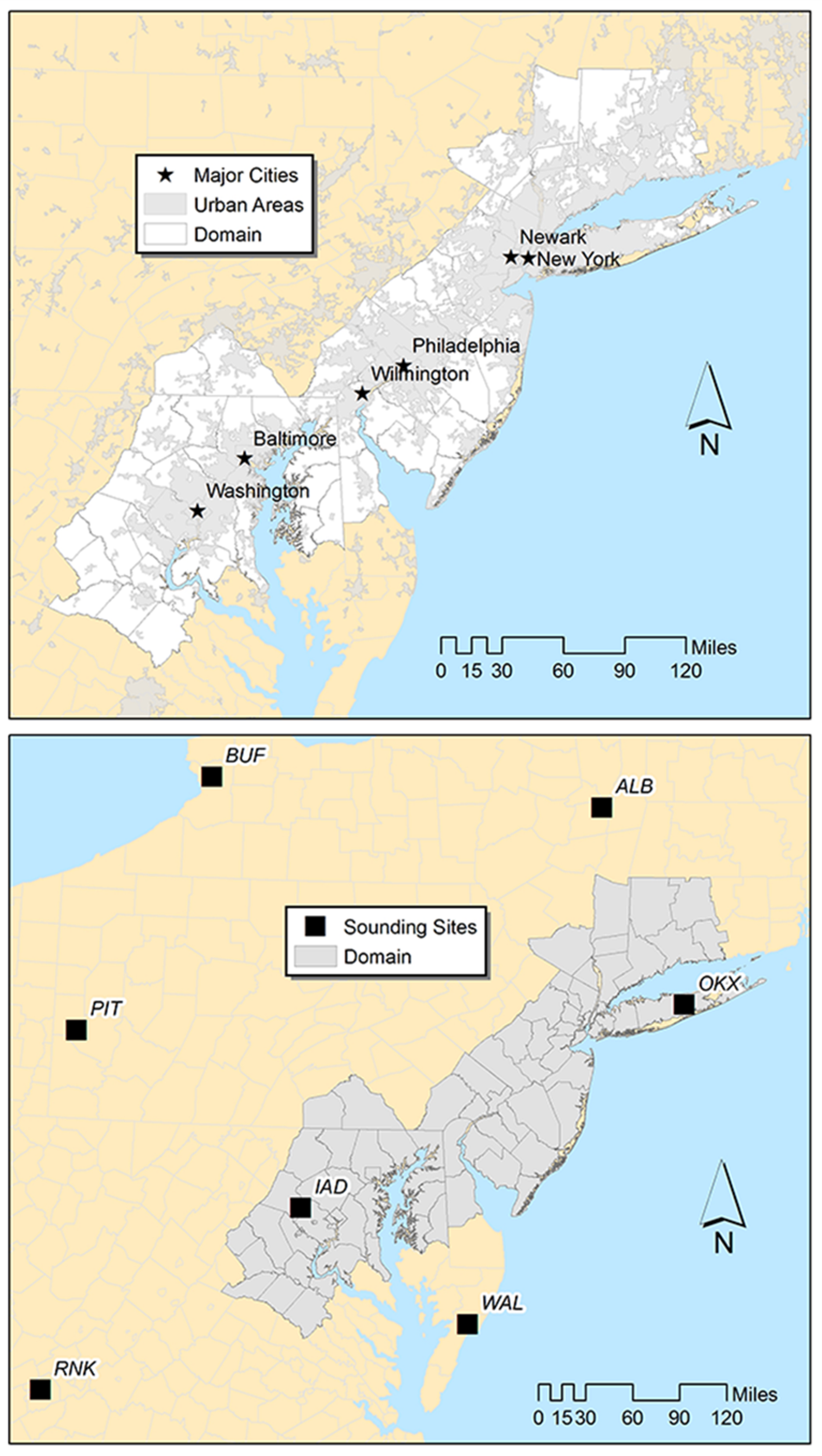
Established observational networks in the Northeast United States do not provide sufficient temporal or spatial sampling of the atmosphere in order to fully represent the evolution and/or occurrence of mesoscale features. Figure 1, adopted from Johnson and Shepherd [14], shows an example of this deficit in upper air data over the Northeastern United States. Gridded reanalysis datasets, such as the North American regional reanalysis (NARR) at a horizontal 32-km grid resolution, are too coarse for urban scale analysis.

3.1. Domain

In this paper, a single date was chosen to focus primarily on the impact of various land use and land cover changes on the lower atmospheric profile. Johnson and Shepherd [14] provide a comprehensive climatology capable of advanced filtering of surface observations over the Northeastern United States from 1995 to 2006. The spatial domain adopted from that dataset centers on the Northeastern United States extends from Northern Virginia to Southern Connecticut and encompasses the major metropolitan areas of Washington, DC, Baltimore, MD, Philadelphia, PA, and New York, NY. The climatology investigated trends in long-term climate data. Even though the study primarily focused on aggregated data trends, the original quality controlled local climatological data (QCLCD [22]) was retained for each day, month, and year within the study period. Within this dataset, four precipitation type categories are provided—all rain, all snow, mixed (inclusive of any form of non-convective, frozen precipitation except all snow), and unknown. An unknown event is indicated when an automated observing station cannot determine the precipitation type and is often associated with sleet and frozen pellets [23]. Each date is filtered by the number of precipitation reports and precipitation type; the dates with the highest number of mixed and unknown precipitation types were identified. The following factors were considered in selecting 6 February 2004 for numerical simulation in this case study:

• Number of mixed and unknown precipitation reports: The most unique mixed and unknown reports within the domain were observed on the single calendar date of 6 February 2004 (329 mixed/unknown, 328 rain, and 39 snow station reports).
• Conditions favorable for the maintenance of the urban heat island: According to Oke [17], the urban heat island is maximized during periods where ū_sfc > 5 ms⁻¹; this date is selected for further scrutiny in this case study.
• Omission of large-scale synoptic systems: Due to the proximity of the domain to the Atlantic Ocean, large-scale synoptic systems capable of advecting large quantities of heat, moisture, and momentum are excluded. (This criterion is executed effectively by implementing Oke’s ū_sfc > 5 ms⁻¹.)

3.2. Methods

Station data is useful when available but is not temporally and spatially sufficient in all dimensions at a scale necessary to examine a singular event; a numerical model simulation is appropriate. The National Center for Atmospheric Research’s (NCAR’s) weather research and forecasting model (WRF) has been utilized by many atmospheric scientists to simulate idealized and real-world phenomena. WRF is a fully compressible, nonhydrostatic, mesoscale forecast model [24]. This study will use WRF model simulations to determine the spatial and temporal effects of specific urban cluster configurations on precipitation distribution and type.

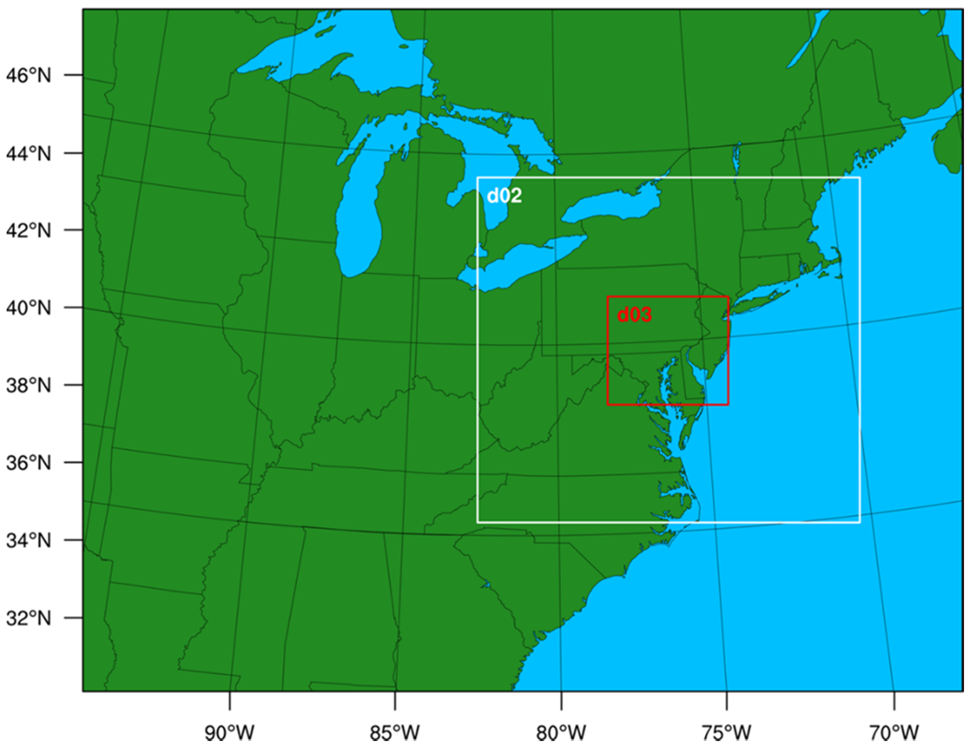
WRF-ARW (advanced research WRF) version 3.8.1 is run in a framework of three two-way nested domains. From the outermost to innermost, the domains, shown in Figure 2, have horizontal grid resolutions of 10, 3.3, and 1.1 km, respectively.

The initial conditions are forced by the North American Regional Reanalysis (NARR), which has a 32-km horizontal resolution [25]. The terrain is provided by the United States Geological Survey Global 30 Arc-second elevation digital elevation model. A summary of the physics and dynamics options are shown in

Table 1. Selected weather research and forecasting model, advanced research WRF version, physics and dynamics namelist options.

WRF Physics and Dynamics Options
Microphysics	Thompson et al. [26]
Longwave radiation	CAM 3 [27]
Shortwave radiation	CAM 3 [27]
Surface layer	Monin-Obukhov (MM5) [28]
Land surface	Noah Land Surface Model [29,30]
Urban surface	Building Environment Parameterization [31]
Planetary boundary layer	BouLac [32]
Cumulus parameterization	Old Simplified Arakawa-Schubert Scheme [33]

.

The model configurations are consistent with other WRF studies of winter precipitation [34,35]. The microphysics is the Thompson et al. [26] scheme. The shortwave and longwave radiation schemes are adopted from the NCAR Community Atmosphere Model version 3.0 (CAM 3) [27]. Land surface physics are taken from the Noah land surface model [36]. An updated version of the MM5 similarity-based surface layer scheme was used [29,30]. The innermost domain (upon which all analysis is conducted) was simulated every six (6) seconds and saved to output every one hour.

Two deviations arose due to the urban focus here. Identifying the urban plume is important when determining precipitation type. The urban surface physics play a key role in the generation of this feature by the model. The building effect parameterization by Martilli et al. [31] uses a multilevel approach in determining response as opposed to the slab-like approach of the urban canopy model option detailed in Chen et al. [37] and is adopted in this study. This scheme is designed to work only with the BouLac planetary boundary layer physics scheme [32]. The total runtime, or time length from the model start to termination, was 117 h beginning at 0000Z on 4 February 2004.

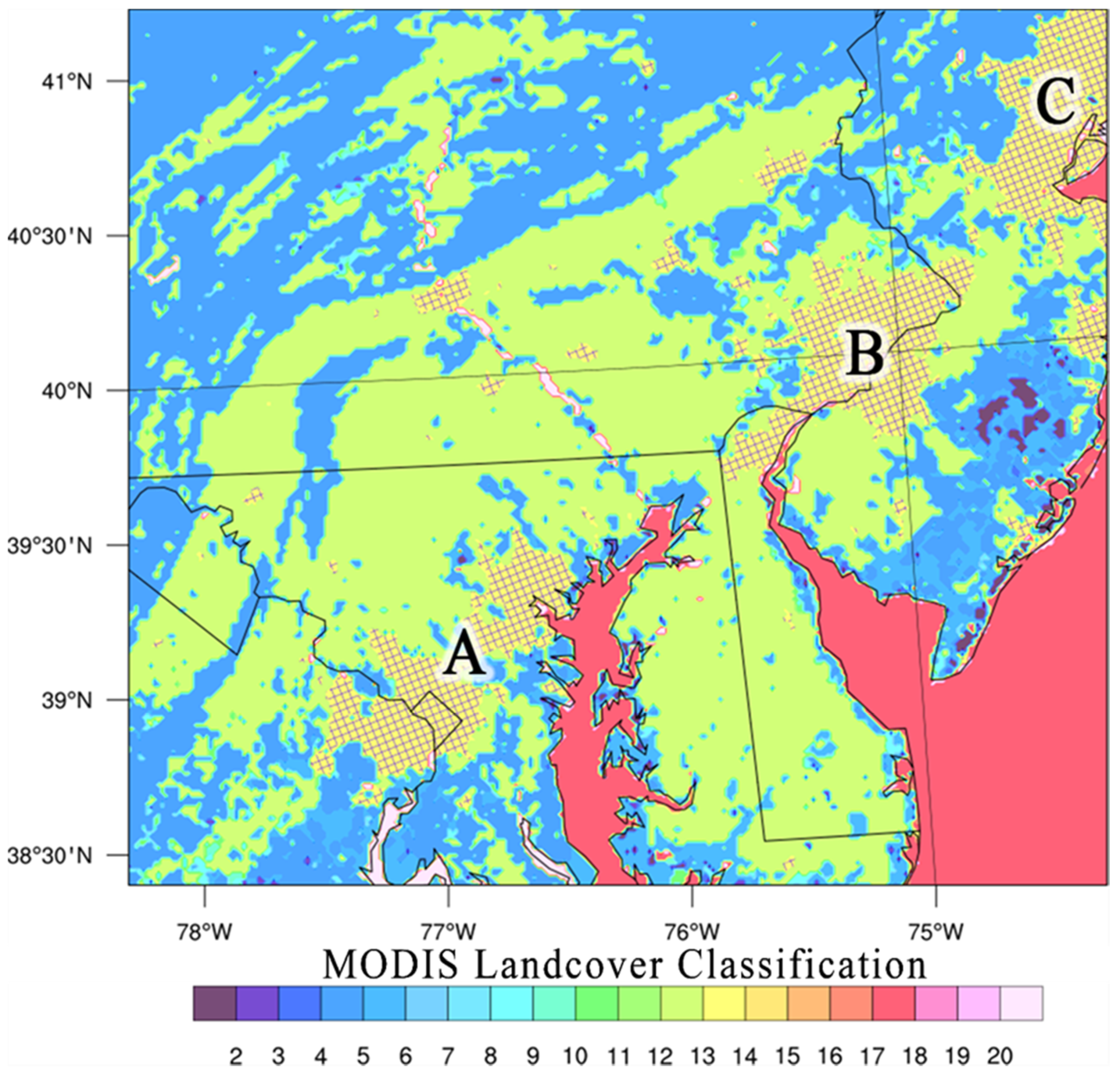
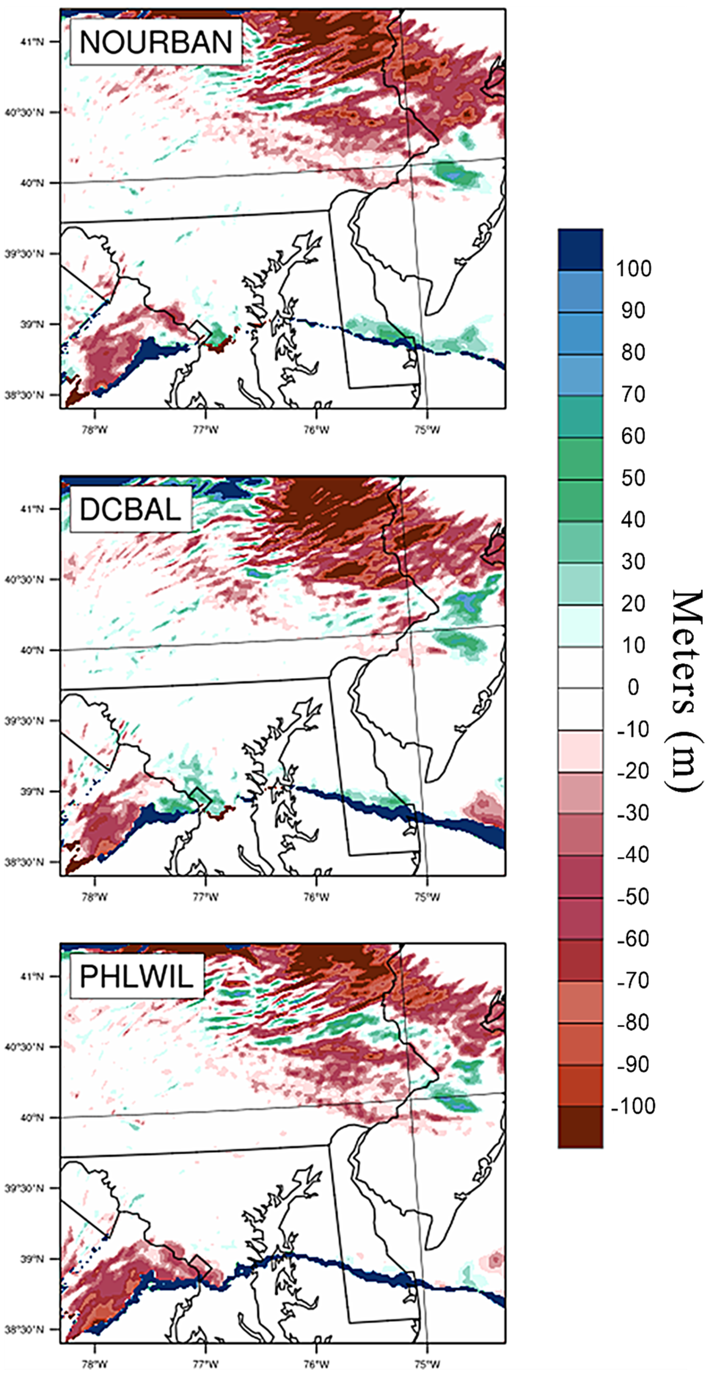
The methodology focuses on the response of a transitional precipitation, synoptic event to variations in the moderate resolution imaging spectroradiometer (MODIS) land use index (and the corresponding LU_INDEX variable in the WRF-ARW model output). The modifications to LU_INDEX occur following the preprocessing phase of the model simulations and are limited to the innermost domain. In all modification schema, grids classified as urban are replaced with deciduous forest, which is the predominant and historical background land cover excluding man-made croplands. The eight simulations with unique LU_INDEX configurations are the following: a control with the original MODIS land cover including all urban classifications, a NOURBAN run with all urban grids removed, and scenarios replacing three representative urban clusters centered on:

• Washington, District of Columbia and Baltimore, Maryland (DCBAL),
• Philadelphia, Pennsylvania and Wilmington, Delaware (PHLWIL), and,
• New York City, New York (NYC).

Spurious urban land cover grids within the rectangular bounds of each cluster are also removed in the analysis. Figure 3 shows the clusters and the affected regions. The three urban land cover areas resulted in six unique scenarios, where one or two of the other metropolitan areas were removed and the other(s) remained. Those configurations are as follows:

1.

DCBAL (PHLWIL and NYC remain),

2.

PHLWIL (DC and NYC remain),

3.

NYC (DC and PHLWIL remain),

4.

DCPHL (NYC remains),

5.

PHLNYC (DC remains), and,

6.

DCNYC (PHLWIL remains).

4. Results

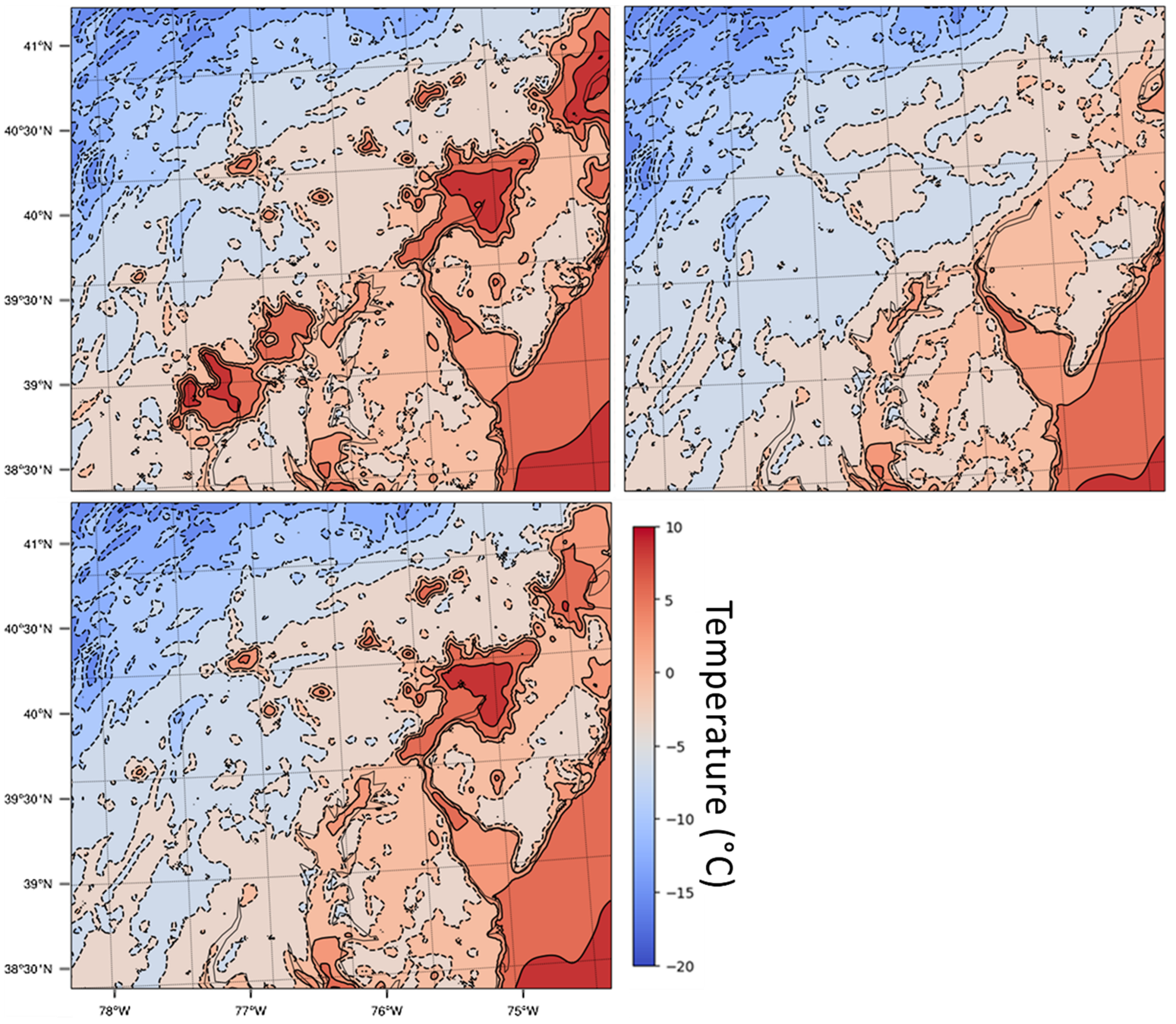
All the following analyses describe the simulated WRF-ARW output data from 0800 UTC on 5 February 2004 to 2100 UTC on 8 February 2004. The simulations yielded 118 hourly time steps. The results presented here are filtered to those immediately preceding and following the onset of precipitation in order to determine the effects of minimally disrupted UHIs throughout the domain. Figure 4 shows the control, NOURBAN, and DCBAL 2-m temperatures, T_2m, just prior to the onset of measurable precipitation at 0000 UTC on 6 February 2004. The urban clusters of DCBAL, PHLWIL, and NYC are easily identifiable with T_2m that is 10 °C warmer than surrounding rural areas that are generally near 0 °C. Surface temperatures have a particularly strong co-located response to land cover changes, which are evident in NOURBAN, DCBAL, and PHLWIL with most replaced pixels showing T_2m ≤ 0 °C. This difference in T_2m would result in varying observations of rain versus freezing rain in control and modified runs, respectively, the vertical temperature profile notwithstanding. Large UHI magnitudes are possible in the temperate broadleaf forest biomes dominating the study domain. Using 8-day composite MODIS-Aqua land surface temperature, Imhoff et al. [38] observed mean summer daytime UHI over 9 °C in Baltimore, MD with mean winter daytime UHI lagging at 3 °C. Under ideal conditions, winter UHI magnitudes can be much higher. For example, winter UHIs in the Arctic reach 11 °C despite an average seasonal urban–rural temperature difference of 1.9 °C [39].

A key objective of this project was to determine the impact of varying urban land cover with respect to urban, suburban, and nearby ex-urban areas. Referencing Figure 3, many of the areas classified as urban varied in density of impervious surfaces. For the purposes of this study, the urban land cover class will approximate urban, suburban, and ex-urban land surfaces. A domain subset was created based on the control urban land cover pixel, LU_INDEX = 13, hereafter referred to as the urban mask, and was applied across output for each land cover configuration.

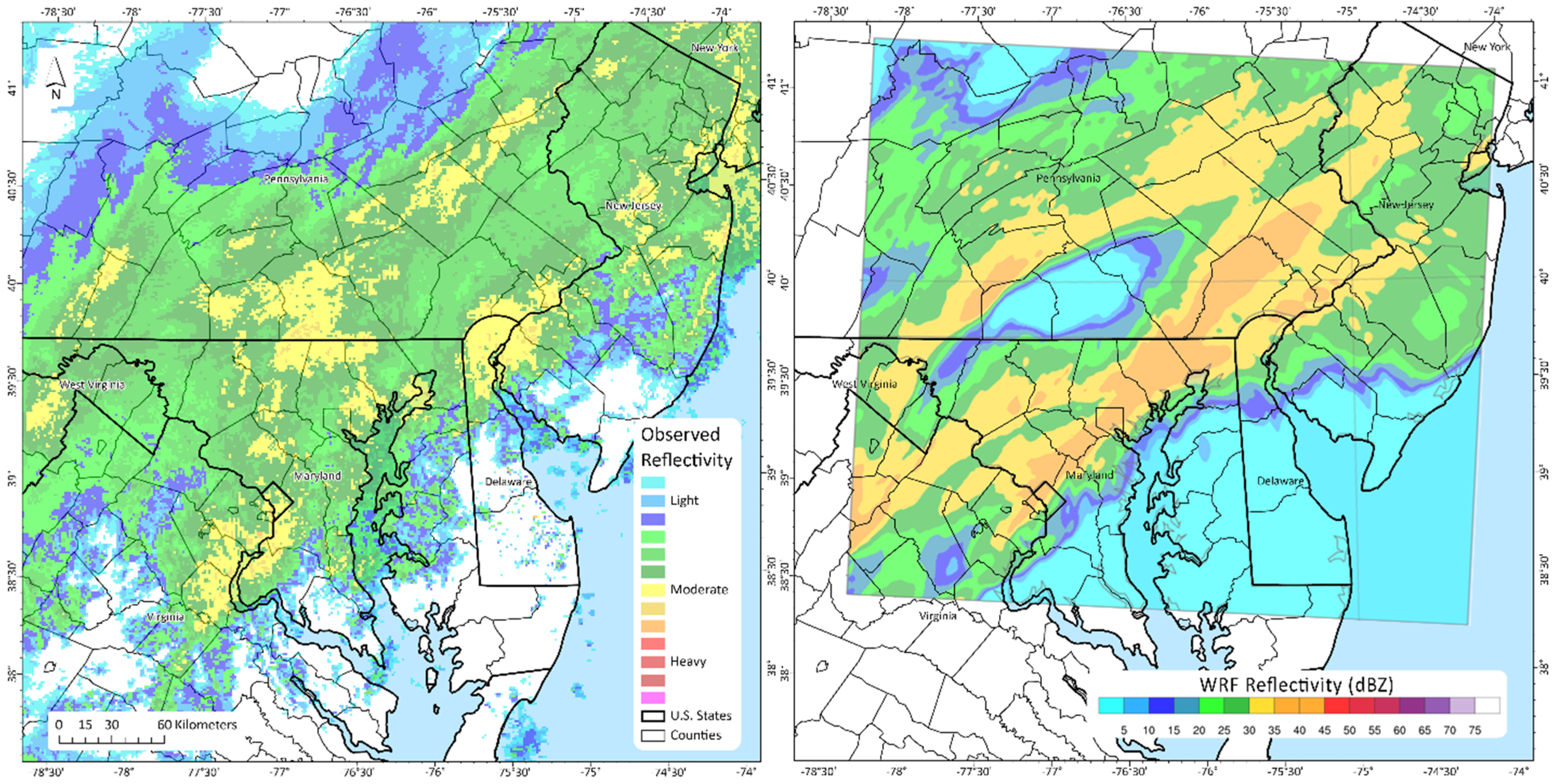
This study was not only concerned with the land surface schema but with its relevance to cold-season precipitation. Qualitative validation of the control simulation for precipitation reflectivity is based on composite radar data obtained from the following National Oceanic and Atmospheric Administration (NOAA)-operated, WSR-88D radar sites near and inside the domain:

• KLWX (Sterling, VA, 38.99, −77.40);
• KDOX (Ellendale, DE, 38.83, −75.44);
• KCCX (Philipsburg, PA, 41.00, −78.01);
• KDIX (Manchester Township, NJ, 39.96, −74.41).

The precipitation timing occurred in two distinct waves or modes. The first was brief and entered the domain around 0000 UTC on 6 February (not shown) and the second, more significant period approached the urban corridor around 1800 UTC on 6 February. Figure 5 shows a comparison of observed precipitation from the NOAA radar sites and the derived reflectivity from the control simulation. The timing and spatial coverage of precipitation is presented well. There are some issues with modeled areal coverage of the highest precipitation rates compared to observations, but the upper limit of precipitation intensity is captured well. It is useful to note that model simulations rarely produce every detail of the quantitative precipitation field. Since precipitation is heterogeneous, unlike more slowly evolving fields like temperature and wind, the simulations depend heavily on model-specific factors (i.e., microphysics, resolution, domain selection, initial conditions, etc.). A review of modeled surface temperatures is also consistent with station-based observations. Considering the temperature-sensitive nature of the BLUHI and the appropriate simulation of precipitation timing, these two factors are deemed to be sufficient. Figure 5 shows a comparison of the observed Doppler composite over the domain and the simulated reflectivity at 1800 UTC on 6 February 2004.

Measurable precipitation is modeled at a minimum of one grid point in the urban mask at 70 unique, hourly time steps across all domain configurations albeit at similar, but non-uniform, distributions. For example, DCPHL has measurable precipitation in 69 of 118 h. The two modes of precipitation are observed in the model runs with the first beginning after the primary onset, 0000 UTC on 6 February 2004. Two separate mask categories with respect to precipitation are created from the urban mask. The first is a precipitation mask for the aforementioned 70 hourly time steps; the second is a subset of the precipitation mask but begins at the primary onset (N_times = 58). The precipitation and onset subsets will be referenced accordingly.

Weather and climate data are often shown to lack spatial independence due to their geographical nature and the seamless connectivity of the atmosphere. For the urban mask, Kolmogorov–Smirnov normality testing and analysis of linear regression model residuals confirmed non-parametric distribution and spatial dependence, respectively, of all variables of interest for all time steps (not shown). Considering the non-parametric distributions, traditional Student’s t tests are not appropriate. Mann–Whitney U tests over the urban mask tests for differences between the control and modified run variables during all available times and, separately, periods of measurable precipitation (

Table 2. Mann–Whitney U test probability values comparing modified datasets to the control dataset. p-values less than 0.1 (0.05) indicate that the samples are different with greater than 90% (95%) confidence. * Under T_2m, the left column is all times; the right column is during precipitation events after the primary onset at 1800 UTC on 5 February 2004.

	p-Value
	T2m *		Tskin	Mean Snow Depth
NOURBAN	<0.001	0.001	<0.001	<0.001
DCBAL	0.073	0.040	0.052	0.003
PHLWIL	0.069	0.041	0.056	0.007
DCPHL	0.003	0.008
DCNYC	0.011	0.014	0.0088
NYC	0.18	0.081
PHLNYC	0.011	0.012

).

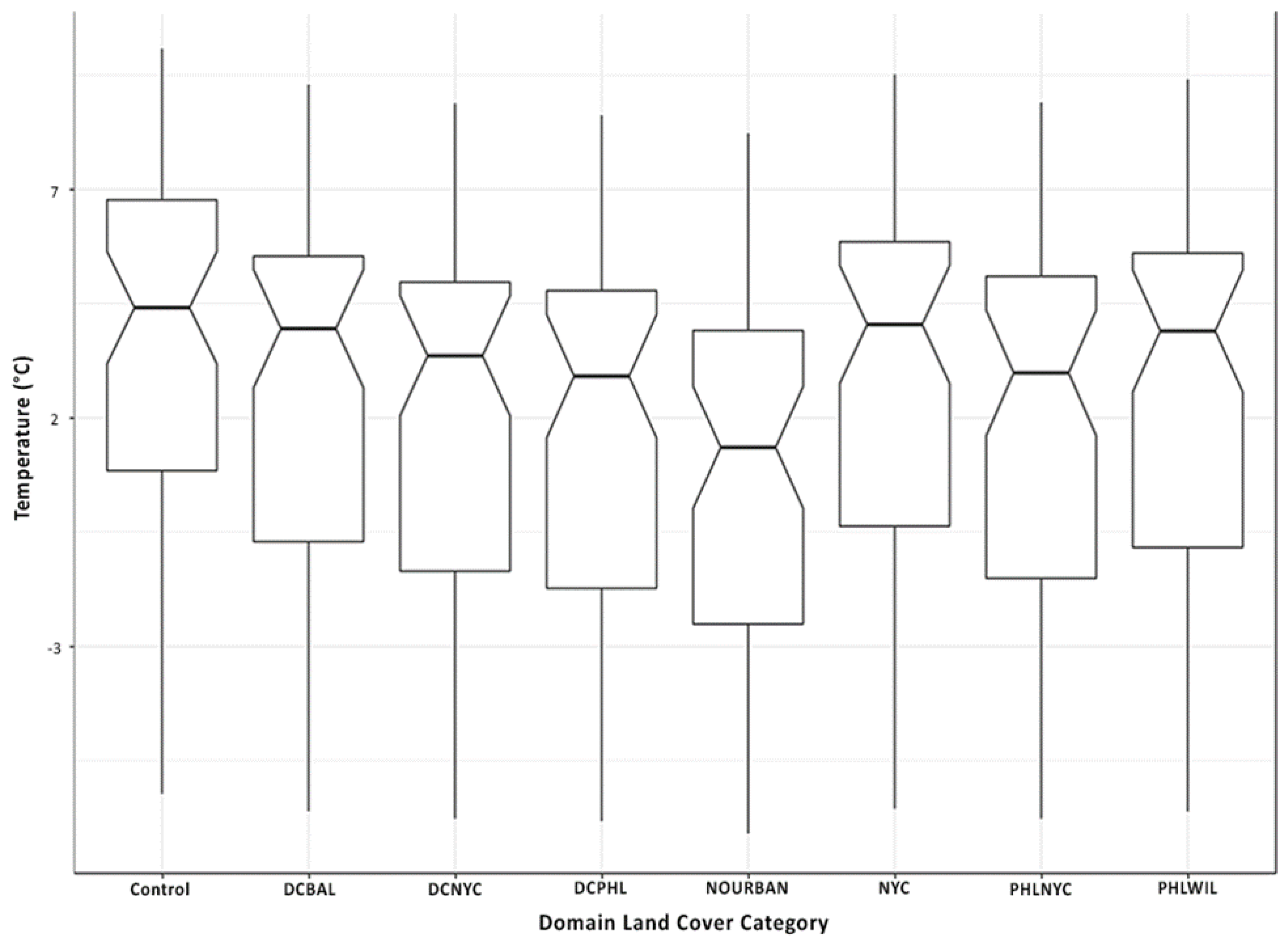
When looking across all times, Mann–Whitney U test values of p < 0.10 for DCBAL, PHLWIL, and NYC and p < 0.05 for NOURBAN, DCNYC, DCPHL, and PHLNYC denote significant differences in T_2m from the control field at 90% and 95% confidence, respectively. Departures in T_2m expand in the precipitation subset where all configurations differed with 95% confidence except NYC (90% confidence). These statistics hold firm in Figure 6, which provides a graphical interpretation of each land cover T_2m distribution in the onset subset. Beyond surface temperature, other factors directly related to impact include the frozen fraction of precipitation and snow depth.

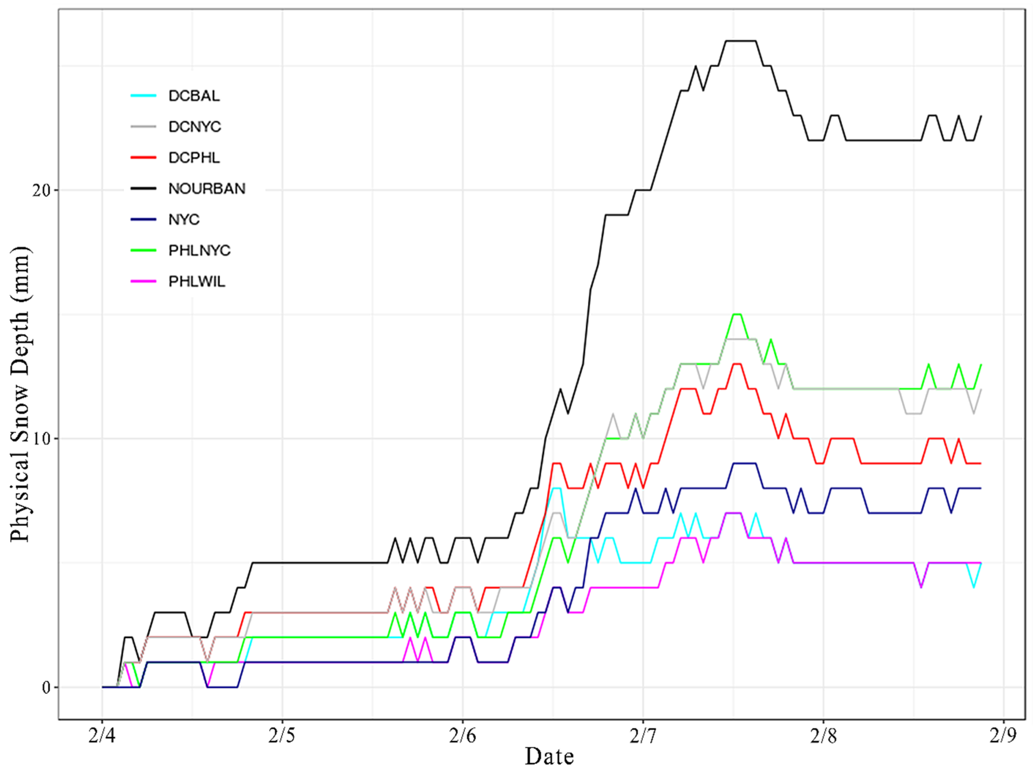
There were no statistical differences between the control and any configuration for the frozen fraction of precipitation, which suggests that there was no difference between the hydrometeor type incident upon the surface. Contrary to this, however, were the findings of mean snow depth across the onset subset (Figure 7). Mean control snow depth was 17.3 mm; mean NOURBAN snow depth was 35.3 mm. All domain configurations differed from the control snow depth at greater than 99% confidence. This introduces a new question—are we experiencing more snow/frozen precipitation in reforested areas, less melting, or some combination of both? This is an area of potential future study.

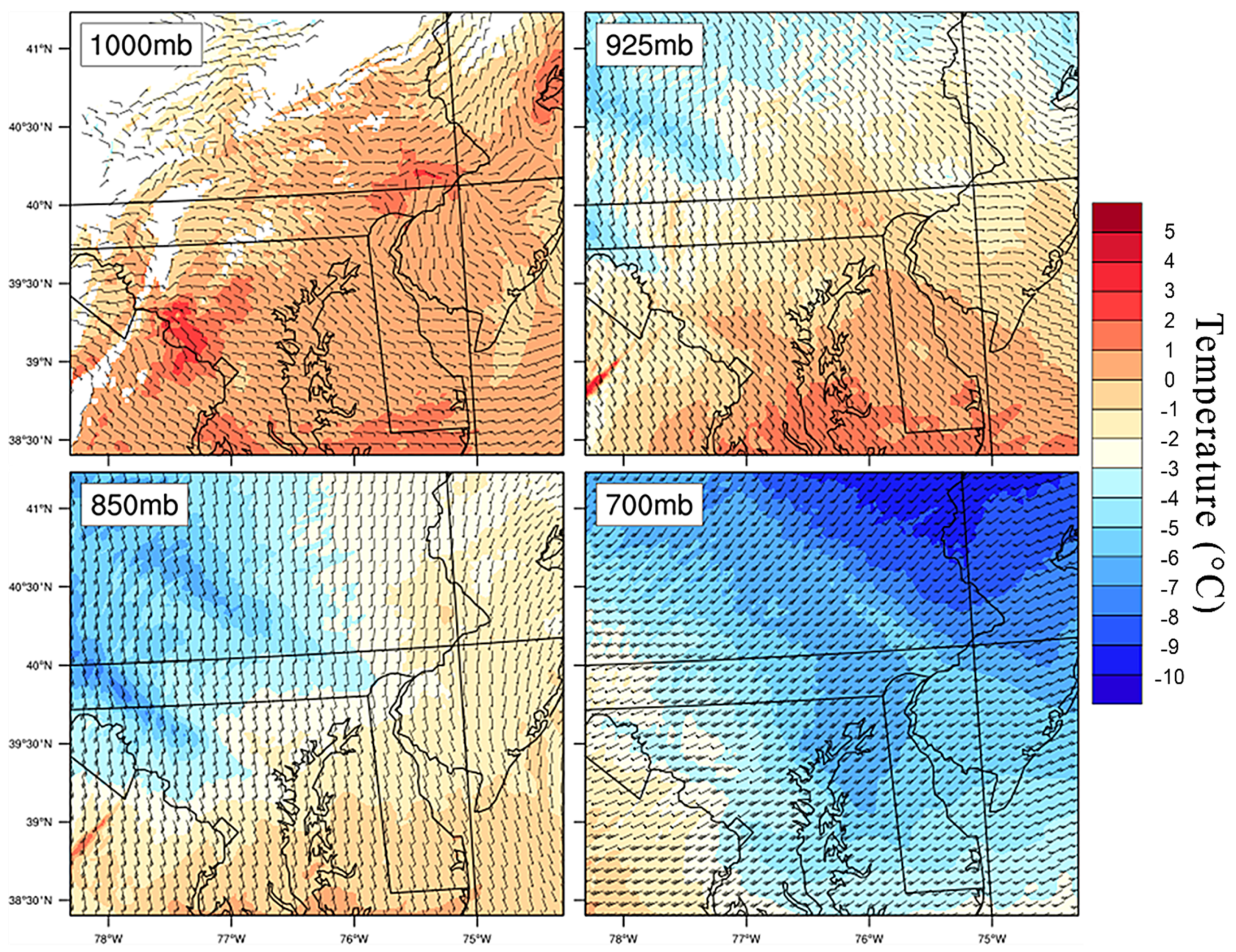
Of the six domain configurations, three were selected for detailed scrutiny with considerations for combined impact of clustering (NOURBAN) and positioning of urban areas (DCBAL and PHLWIL). In determining the precipitation type prior to contact with the surface, the lower atmosphere vertical temperature profile is important. The air temperatures at 1000, 925, 850, and 700 mb at 0000 UTC on 6 February show the control run conditions that are marginal for winter precipitation with T₁₀₀₀ near or above freezing across all metropolitan centers (Figure 8). The influence of the BLUHI appeared to diminish substantially above 925 mb where differences in temperature were mostly indistinguishable between the control and NOURBAN runs (Figure 9).

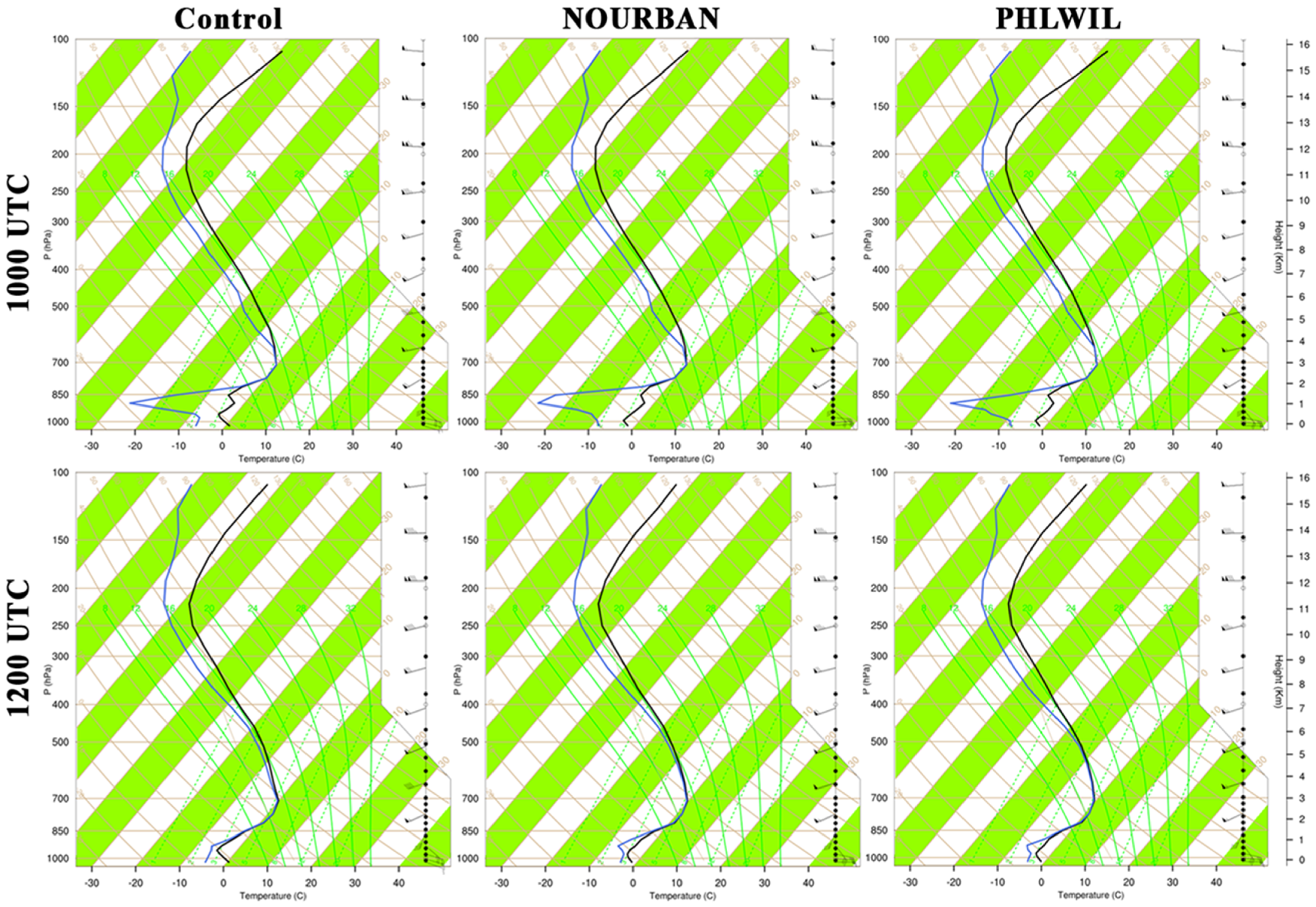
Figure 10 compares the vertical profile in the control, NOURBAN, DCBAL, and PHLWIL runs at Philadelphia, PA from 1000 to 1200 UTC on 6 February. As anticipated, surface temperatures in the NOURBAN (T_sfc,NU) simulation were less than those in the control (T_sfc,ctl). This is due to an increase in natural land cover and a decrease in anthropogenic heat and impervious surfaces. Dewpoint changes were not immediately evident at the surface. Note the evolution of the lower troposphere, particularly where T_sfc,NU < T_sfc,ctl and T_d,NU ≈ T_d,ctl (where ≈ is ‘approximately equals’) conceptually led to higher relative humidity, lower lifting condensation levels, and, consequently, less melting, evaporation, and sublimation of hydrometeors in NOURBAN. This point observation is representative when comparing other locales (PHLWIL is shown) across the domain subset.

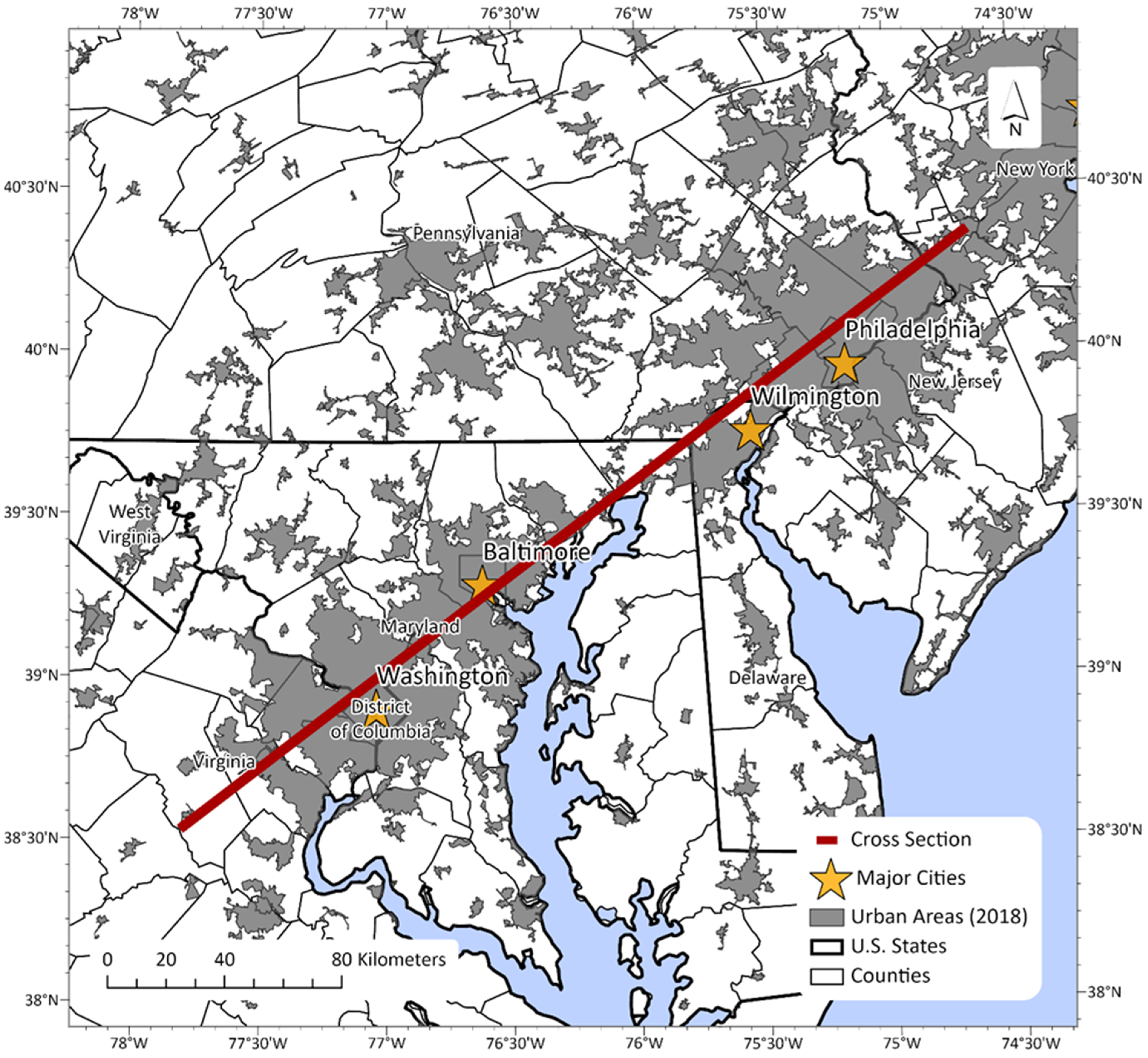
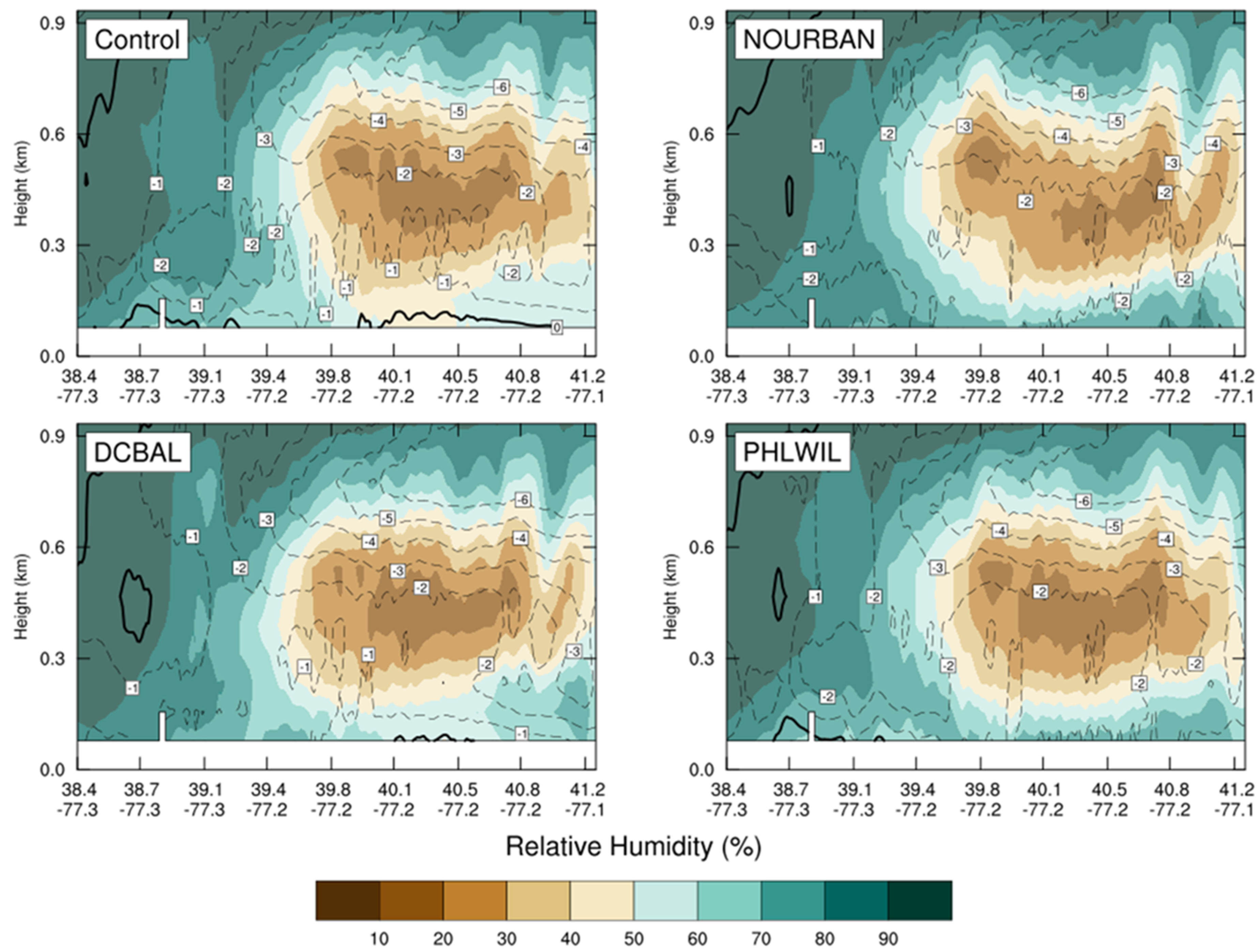
Another perspective on this departure can be seen via vertical cross-sections, as depicted in Figure 11, of temperature and relative humidity (Figure 12 and Figure 13). This transect originates in Northern Virginia just southwest of Washington, DC (38.9° N), travels northeast through Baltimore, MD (39.2° N) and Philadelphia, PA (40.0° N), and ends at Princeton, NJ. While only one time slot near 0800 UTC is shown, all hourly steps were generated. A warmer layer of air, T > 0 °C, entered the domain from the southwest, centered near 2 km above the surface, and overran the colder air at the surface. By 0800 UTC, the warm layer or trowel had traveled approximately two-thirds of the cross-section length and had deepened to just under 2 km thick in the control simulation. At the surface (Figure 14), temperatures above freezing were present coincidently with Washington, Baltimore, and Philadelphia; these represent each city’s BLUHI. The warmer surface temperatures were no longer present in the NOURBAN simulation and were reduced in the remaining two runs over the “reforested” cities by 2–3 °C. 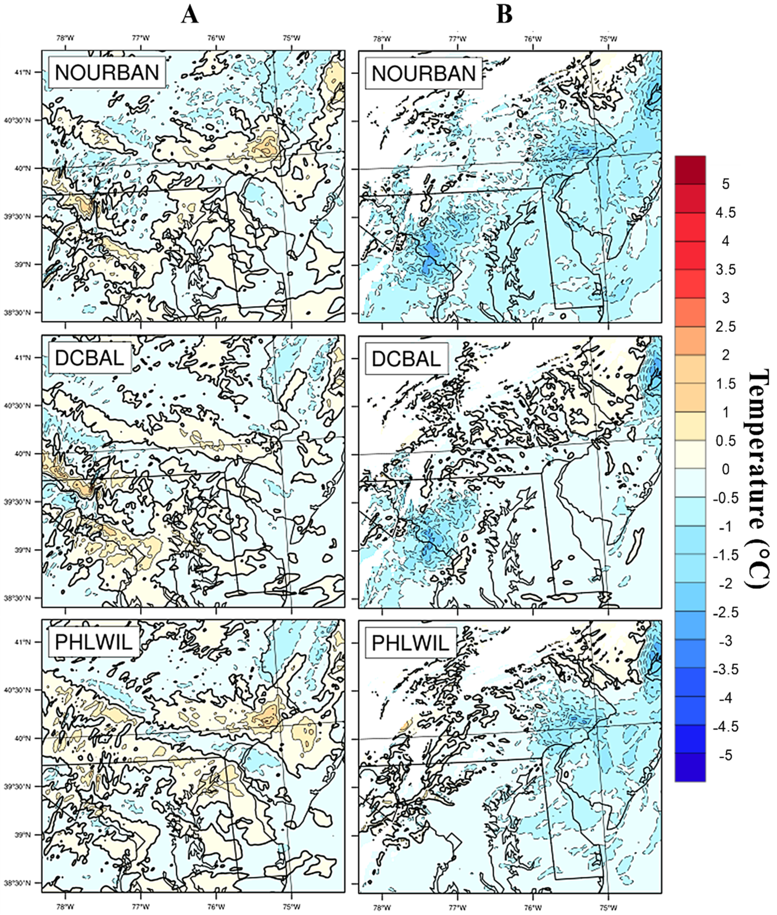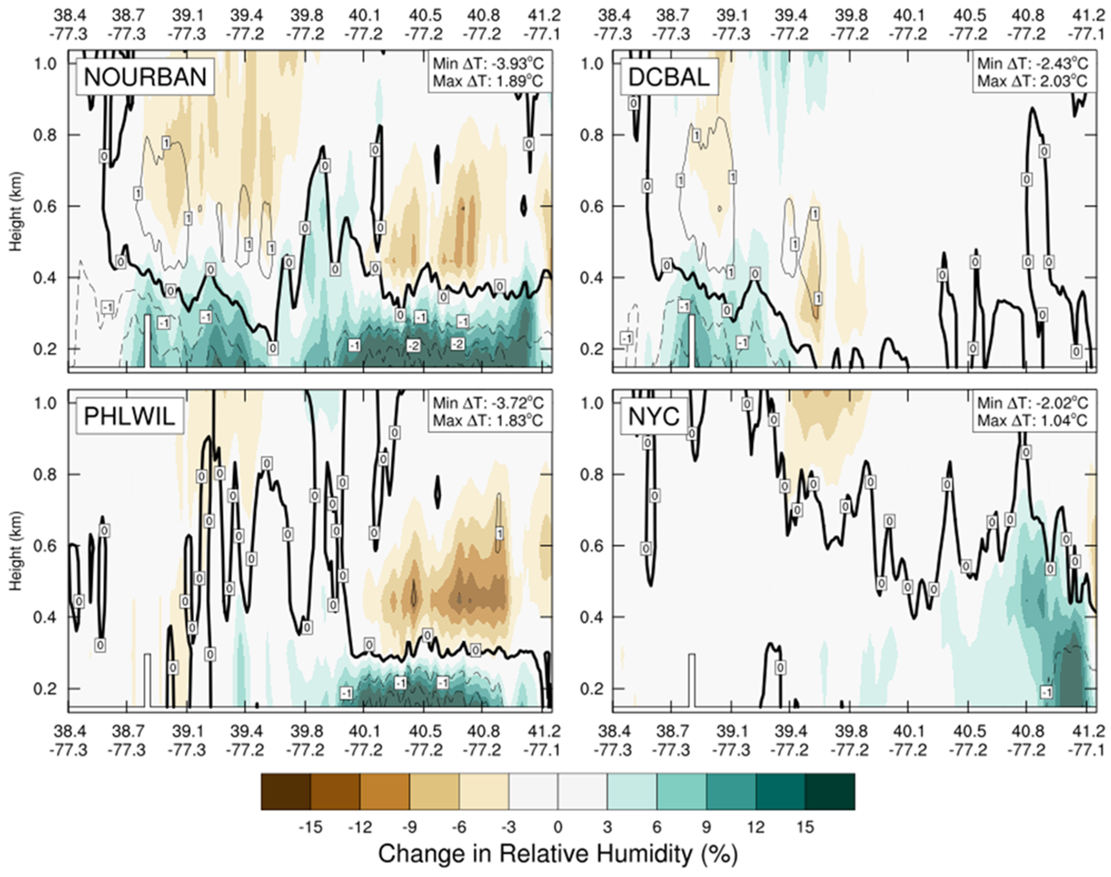Figure 15 displays the differences in air temperature and relative humidity from the control simulation. Interestingly, Figure 15 shows the magnitude of the DC-Baltimore BLUHI in the poleward direction was slightly reduced even when its urban surface remained in the land cover scheme but PHLWIL was removed. This result implies that at least some component of the DC-Baltimore UHI is related to the existence of Philadelphia and Wilmington even though the two urban clusters were not directly adjacent to one another.

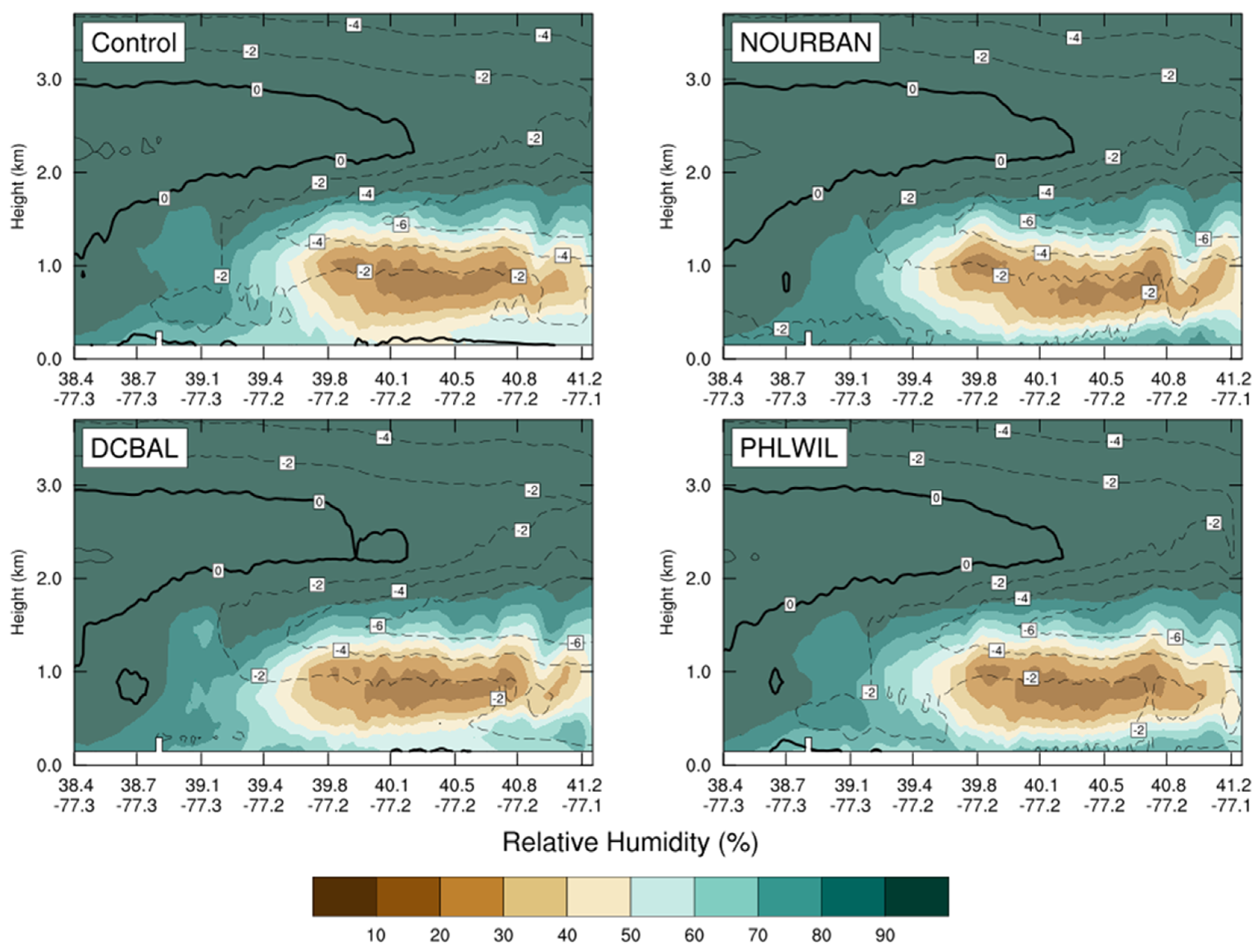
These relationships are also reflected in the available moisture at the surface. At the time step shown in Figure 13 and Figure 14, precipitation is beginning in the southernmost (or left) part of the cross-section where high relative humidities are observed throughout the column. A very dry layer of air is present in the northern half of the domain near the surface in the control. Layers of lower humidity are often responsible for evaporation and sublimation of light stratiform precipitation that falls from saturated layers above. Evaporation is a cooling process due to the significant latent heat transfer from the surrounding atmosphere to facilitate the phase change. This dry layer slowly progressed northeast over time in front of the trowel. While the magnitude of the dry layer remained consistent, the surface was markedly less dry in the NOURBAN run and other runs following the previously described temperature pattern. The relative humidity at the surface around the urbanized DC-Baltimore area was higher when PHLWIL was replaced, resulting in a shallower dry layer. The water vapor mixing ratio (not pictured) was also incrementally higher in the same scenario. Once again, this suggests a regional response to urbanization existed beyond the local urban–rural interface. The implications for this process on precipitation type are complicated as a thinner dry layer could actually lead to more observed surface precipitation due to less evaporation while simultaneously decreasing the cooling from the same process near the surface. There was also a curious fall in relative humidity above approximately 500 m over reforested areas that coincided with increases in humidities near the surface. Future research might focus on the physical causes for these humidity dipoles in model simulations, the implications of near surface relative humidity, the magnitude of the urban dry island, and the response of precipitation in various scenarios.

5. Discussion and Concluding Remarks

WRF-ARW simulations on a fine spatial scale such as a 1.1-km horizontal grid provide a unique perspective on urbanization and the atmospheric response. Few studies have attempted to create these simulations to monitor these responses outside of warm-season convection and even fewer, if any, focus strictly on winter precipitation. The results presented in the paper show that a variety of features may be studied but also highlight the limitations of current numerical capabilities. For example, Figure 15 shows the departure of LCL height in modified land cover simulations from the control, MODIS land cover simulation. While the results were negligible outside of the northern and southwestern regions where cloud bases were lower than the control run and artificial pseudo-linear stretches of higher LCLs are seen across all three figures. This may be due to surface-based convective rolls present in conditionally unstable WRF simulations and described by Bryan et al. [40]. If these are indeed represented as such, this scenario should not exist in these simulations considering the lack of instability during the synoptic setup and, more generally, due to seasonality. Despite this abnormality, there were a few areas that provide insight into urbanization and evolution of winter precipitation.

For this case study, there were clear differences near the surface between the urbanized control and modified land cover methods. When urbanization was completely removed, those immediate (or previously urban) areas were on average approximately 2.3 °C cooler and indistinguishable from surrounding rural surface temperatures. These anomalies increased to near 2.6 °C during times in which measurable precipitation was observed within the domain. Skin temperatures decreased by more than 4.8 °C from control in similar situations. Combined with the growing disparity in snow depth as the level and contiguity of urbanization changes from the control to interrupted to complete reforestation, it is evident that the addition of impervious surfaces changed the baseline thermal makeup and, thus, climate of the region. This is most evident in the comparison of the 2-m temperature where distinctions from the modern land surface are shown. Single “reforested” cities or clusters differed confidently from the modern land surface temperature at significant levels, yet, when multiple clusters were reforested, confidence increased by a factor of 10. This reinforces the work by Debbage and Shepherd [41] that suggests contiguity of urbanization plays a significant and potentially more of a role in the occurrence of UHIs than urban sprawl or density. Considering Theriault’s findings that require only subtle temperature and dewpoint deviations to change precipitation type, these alterations are indeed sufficient to facilitate such a change even if only present in a very shallow layer.

These findings are somewhat intuitive, as removing heat sinks (and subsequent sources) should result in lower temperatures, increasing observations of freezing rain, and accumulating snowfall. Moving forward, the more interesting question might be to what degree this occurs and how can we design our cities to be less susceptible to “surprise” events where urbanization does not play a strong role in the modification of precipitation type. While this study did not address that specific question, it did suggest that there are factors at play in the form of urban morphology and spatial configuration that could be important. A single case study in a specific scenario and domain can be informative but primarily serves as a platform to develop more relevant questions. Figure 10 and Figure 14 both show that dewpoints at the surface did not change from the control, or urbanized, to the reforested runs. Considering the increase in vegetation in reforested runs, an increase in moisture near the surface was expected. So, while the lowest levels of the atmosphere have higher relative humidities in reforested runs, it is due to the decrease in surface temperatures and not an increase in actual water vapor content. Is this true in other scenarios and/or urban environments? What are the impacts outside of ideal urban heat island situations? Why are transient, light precipitation events adversely impactful and more difficult to manage compared to larger, high-profile events? Are the presence or absence of impervious surfaces enough to determine regional climate impacts or is configuration and orientation important? This paper aimed to determine the assessment utility of urban land cover modification in winter precipitation events. In practice, the answer is beyond the scope of a single case study.

This case study is one of few modeling studies of urban, winter precipitation mechanisms. It also invigorates the discussion of urban landscape or boundary layer interactions as they pertain to winter weather hazards. Furthermore, it builds upon the body of work detailed by Liu and Niyogi [20] and perpetuates the urban cluster framework that considers the collective climatological impact of cities and pushes urban hydrometeorological research closer to real-world applications. Inevitably, these questions and others require an interdisciplinary approach that considers, not only forecasting and model capabilities but city planning and social science perspectives. Investigations of multiple storms and case studies are also prudent. There are inherent limitations that warrant further dialogue, including, but not limited to, the efficacy of WRF-ARW, the available schema, and their viability in discerning urban-scale phenomena with the sensitivity of precipitation type. The heterogeneity of land cover and land use must be parameterized in current predictive models, this is part of a feedback cycle that is likely important in thermally sensitive transitional events. Decreased wind speeds and increased cloud cover during precipitation events as presented in this case study may present conflicting effects on UHI magnitude causing event timing to play a role [42]. Most simulations in urban climate invoke ‘all or nothing’ approaches, removing and replacing entire categories of coarsely classified land cover and land use. More sophisticated approaches might utilize more heterogeneous land cover and invoke urban parameterization schemes capable of processing the associated atmospheric responses. One component that limits this approach is the standard urban configuration of WRF-ARW itself; customized configurations and parameterizations are likely needed. Finally, the role of observations is crucial in understanding the urban morphology, atmospheric response, verification and validation, and providing accurate boundary conditions for model simulations. Despite increasing interconnectivity and implementation of smart grids, much atmospheric data remains either convoluted or a proprietary, and thus, inaccessible to researchers that rely upon open access platforms.