ULF Activity in the Earth Environment: Penetration of Electric Field from the Near-Ground Source to the Ionosphere under Different Configurations of the Geomagnetic Field

Abstract

The problem with the penetration of electric fields from atmospheric near-Earth electric current sources to the ionosphere is investigated both within the dynamic simulations of the Maxwell equations in the frequency domain and within the simplified quasi-electrostatic approach. Two cases of the geomagnetic field lines are considered. The first case is the penetration of the geomagnetic field lines deeply into the magnetosphere (open field lines), whereas the second one is the return of these lines into the Earth’s surface (closed field lines). The proper boundary conditions are formulated. It is demonstrated that in the case of the open field lines the results of the dynamic simulations differ essentially from the quasi-electrostatic approach, which is not valid there. In the case of the closed field lines, the results of simulations are practically the same both within the dynamic approach and within the quasi-electrostatic one. From realistic values of the densities of atmospheric electric currents ~0.1 µA/m², the values of the electric fields within the ionosphere F-layer may reach about 1–10 mV/m.

1. Introduction

The problem of the lithosphere (Earth)-atmosphere-ionosphere-magnetosphere (LEAIM) coupling has been investigated for a long time [1,2,3,4,5,6,7,8,9,10,11,12,13,14,15,16,17,18,19,20,21,22] with special attention to the preparation of natural hazards and their ionospheric effects. In particular, this concerns earthquakes (EQs), tropical cyclones, and volcanic eruptions [1,2,3].

The hypotheses have been formulated on electrostatic [2,4,11,14,17], electrostatic-photochemistry [4,5], quasi-static [15], electromagnetic [15,16,22], acoustic-gravity [6,12,13] and other channels of seismo-ionospheric coupling, including ones of synthetic types. Examples of physical processes making a contribution to the preparation of probable precursors of the natural hazards are radon emanation and charging aerosols [1,2], formation of charge layers in the atmosphere [10], formation of a large electric field in the mesosphere [7,8], variations of very low frequency (VLF) field in the waveguide Earth-Ionosphere [3,5,16,22], total electron content (TEC) variations in the ionosphere [20,21], etc.; these processes, in general, are of synergetic character [6,9,15,18].

For several decades, experimental results have been accumulated and recently generalized, including targeted observations over a number of years, which unambiguously indicate the presence of seismogenic disturbances in TEC, VLF, low frequency (LF) and ultra-low frequency (ULF) ranges of electromagnetic field, surface temperature, outgoing infrared (IR) radiation, chemical potential in the lower atmosphere, ionization anomalies, etc. [2,23,24,25,26,27]. As it was mentioned above, a set of mechanisms of coupling, in particular seismo-ionospheric one, in the LEAIM system has been proposed; in particular electrostatic [28,29], electro-photochemical [5,30], electromagnetic [15,16], mechanical (via Acoustic-Gravity Waves (AGW)) [31] and mixed mechanical-electrical [1,15,24,25,27,32,33] mechanisms have been discussed; at the same time, most likely, that in any of the above options, the observed physical phenomena are provided, accounting for the achieving by the corresponding perturbations the amplitudes, significantly exceeding the noise level, by synergetic processes in active open nonlinear LEAIM system [6,9,15,18,33,34]. Only a synergetic approach allows one to adequately, and therefore necessarily self-consistently, determine the electric field in the lower atmosphere. Moreover, for this, it is necessary to take into account a variety of physical processes, the development of instabilities and their nonlinear limitations [9] in different regions and at different heights in the LEAIM system, as well as boundary conditions, including in the lower atmosphere [15,34]. In this work, as in [15], we do not apply such a self-consistent synergetic approach and focus on the questions formulated below about comparing the dynamic and quasi-electrostatic approaches, and for situations with different configurations of the geomagnetic field. In this work, as in [15], instead of a self-consistent consideration of the motion and dynamics of charged and uncharged components of a plasma-like medium, an external current in the lower atmosphere is specified. Hereinafter, an external current is understood as a current that characterizes a given source, which is not determined by a self-consistent calculation based on the properties of the medium in which the excitations are investigated, but “assigned” and in this sense is “external” in relation to the given system, in which perturbations are sought [35]. The consequence of this is the inevitable rejection of any claims for an adequate determination of the components of the electric field in the region where the external current is specified, i.e., in the lower atmosphere. To emphasize this, in the graphs of the vertical distribution of the electric field components given in Section 3 (Figures 5, 7, and 8), an empty space is left in the region of the lower atmosphere. The external current only simulates the real current generated in the lower atmosphere by all the physical processes taking place in a self-consistent manner, but at the same time, it makes it possible to determine the field penetrating the upper ionosphere/magnetosphere.

In the present paper, we are concentrated on electromagnetic/quasi-static channel of coupling, in particular seismogenic, in the system LEAIM. We consider the electromagnetic/quasi-static perturbations in the ionosphere as a sensitive indicator of the coupling in the system mentioned above. It is interesting to note the electric fields of what orders of magnitude are observed in different regions of the atmosphere-ionosphere and at what altitudes. In the papers [29,36,37] the measurements of the vertical electric field variations with amplitudes of order (1-few) kV/m on the ground level in the region of the preparation of strong earthquakes have been reported. In [7,38] the observations of ionospheric inhomogeneities using MF-HF (Medium Frequency–High Frequency) radar have been made; the results correspond to the presence of an effective source of a mesospheric current or an electric field with amplitude (1-few V/m) [7,38,39]. It is interesting that, as it follows from the results of the numerical modeling, electric fields with amplitude of the same order (1-few V/m) in the mesosphere correspond to the presence of the (seismogenic) vertical electric field on the lithosphere-atmosphere boundary of order (1-few) kV/m [4,36,37,39]. AIP (Advanced Ionospheric Probe) on board of FORMOSAT-5 [40] provided measurements, in particular, of ion velocities. The amplitude of a seismogenic electric field in the ionosphere has been evaluated as a value of order 1 mV/m. Seismogenic plasma bubbles observed in the ionosphere, in accordance with the modeling [6], correspond to the presence of a near-ground external electric current with density ~1 µA/m² and seismogenic electric field of order (few-10) mV/m in the ionosphere. The value of electric field amplitude of the same ordering [15,41] corresponds to the observed variations of order dozens of percent in total electron content (TEC) before strong earthquakes (M > 6) as well.

In our view, the coupling in the LEAIM system should be considered generally as a dynamic problem, including the set of possible instabilities [1,6,7,8,18,42,43,44,45,46,47] due to the dynamic nature of the processes in the lithosphere, atmosphere, ionosphere, and magnetosphere. At least, there are diurnal temporal changes. Thus, either the Maxwell equations or equivalent ones should be used to consider the coupling of near-Earth sources with the non-uniform medium possessing the highly anisotropic conductivity. The proper boundary conditions should be applied both in the lithosphere and in the upper ionosphere/magnetosphere.

This paper is devoted to the theoretical investigation of the penetration of electromagnetic fields into the ionosphere and the magnetosphere from near-Earth current sources under different configurations of the geomagnetic field lines. The first case is the penetration of the geomagnetic field lines deeply into the magnetosphere (open field lines), whereas the second one is the return of these lines into the Earth’s surface (closed field lines). The simulation is dynamic that is based on the equations for the locally horizontal components of the electric field, which are equivalent to the Maxwell ones in the frequency domain. The proper boundary conditions are formulated. They are the radiation ones, i.e., the absence of the ingoing magnetohydrodynamic waves, in the magnetosphere in the case of open field lines. In the case of closed field lines, the boundary conditions should be formulated on the Earth’s surface where the field lines return.

Numerical modeling realizing the algorithm used in present paper based on combined spectral-finite different method [48,49,50].

Also, the problem of the penetration of the electric fields is considered within the quasi-electrostatic approach. It is demonstrated that in the case of open field lines, the results of the dynamic simulations differ essentially from the quasi-electrostatic approach. Moreover, the results within the quasi-electrostatic approximation depend on the position in the magnetosphere, where the upper boundary condition is formulated. In the case of closed field lines, the results of simulations are practically the same both within the dynamic approach and within the quasi-electrostatic one.

2. Basic Equations and Parameters

The main equations used in this paper are the Maxwell equations in the frequency domain.

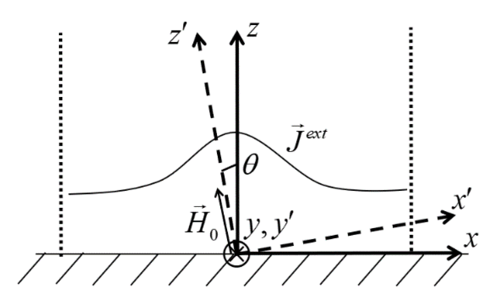
The model uses two coordinate frames, shown in Figure 1, and imaginary side walls, on which zero boundary conditions are formulated. The distance between the imaginary side walls is considered to be much larger than the typical horizontal scale of the “external source” of current in the lower atmosphere ${\overrightarrow{J}}^{ext}$ (see Figure 1 and relation (10)).

The electromagnetic field is sought in the form E, H ~ exp(iωt), where ω is the circular frequency, which is in the ULF range ω ≤ 1 s⁻¹:

$$\begin{array}{l}\overrightarrow{\nabla }\times \overrightarrow{H}=i\frac{\omega }{c}\widehat{\epsilon }(\omega ,z)\cdot \overrightarrow{E}+\frac{4\pi }{c}{\overrightarrow{j}}^{ext}(x,y,z);\\ \overrightarrow{\nabla }\times \overrightarrow{E}=-i\frac{\omega }{c}\overrightarrow{H}.\end{array}$$

(1)

In Equation (1), ${\overrightarrow{j}}^{ext}$ is the density of the external current, $\widehat{\epsilon }(\omega ,z)$ is the dielectric permittivity of the medium. The density of the external current and the field components depend on the frequency and all coordinates x, y, z. It is assumed that the properties of the ionosphere and the lower magnetosphere depend only on the vertical coordinate associated with the Earth’s surface, while in the upper magnetosphere they depend on the coordinate associated with the direction of the geomagnetic field.

In the coordinate frame X’Y’Z’ associated with the geomagnetic field ${\overrightarrow{H}}_0$ the dielectric permittivity tensor has the form [51,52]:

$${\widehat{\epsilon }}^{\prime }\left(\omega ,z\right)=\left(\begin{array}{ccc}{\epsilon }_1& {\epsilon }_h& 0\\ -{\epsilon }_h& {\epsilon }_1& 0\\ 0& 0& {\epsilon }_3\end{array}\right),$$

(2)

where

$$\begin{array}{l}{\epsilon }_1=1-\frac{{\omega }_{pi}{}^2\cdot (\omega -i{\nu }_i)}{({(\omega -i{\nu }_i)}^2-{\omega }_{Hi}{}^2)\cdot \omega }-\frac{{\omega }_{pe}{}^2\cdot (\omega -i{\nu }_e)}{({(\omega -i{\nu }_e)}^2-{\omega }_{He}{}^2)\cdot \omega };\\ {\epsilon }_3=1-\frac{{\omega }_{pi}{}^2}{(\omega -i{\nu }_i)\cdot \omega }-\frac{{\omega }_{pe}{}^2}{(\omega -i{\nu }_e)\cdot \omega };{\epsilon }_h\equiv ig;\\ g=\frac{{\omega }_{pi}{}^2\cdot {\omega }_{Hi}}{({(\omega -i{\nu }_i)}^2-{\omega }_{Hi}{}^2)\cdot \omega }-\frac{{\omega }_{pe}{}^2\cdot {\omega }_{He}}{({(\omega -i{\nu }_e)}^2-{\omega }_{He}{}^2)\cdot \omega }.\end{array}$$

(3)

The following notations are used in relations (3):

$${\omega }_{pe}{}^2=\frac{4\pi e^2{n}_{e0}}{m_e},{\omega }_{pi}{}^2=\frac{4\pi e^2{n}_{e0}}{M_i},{\omega }_{He}=\frac{e{H}_0}{m_{e}c},{\omega }_{Hi}=\frac{e{H}_0}{M_{i}c}.$$

(4)

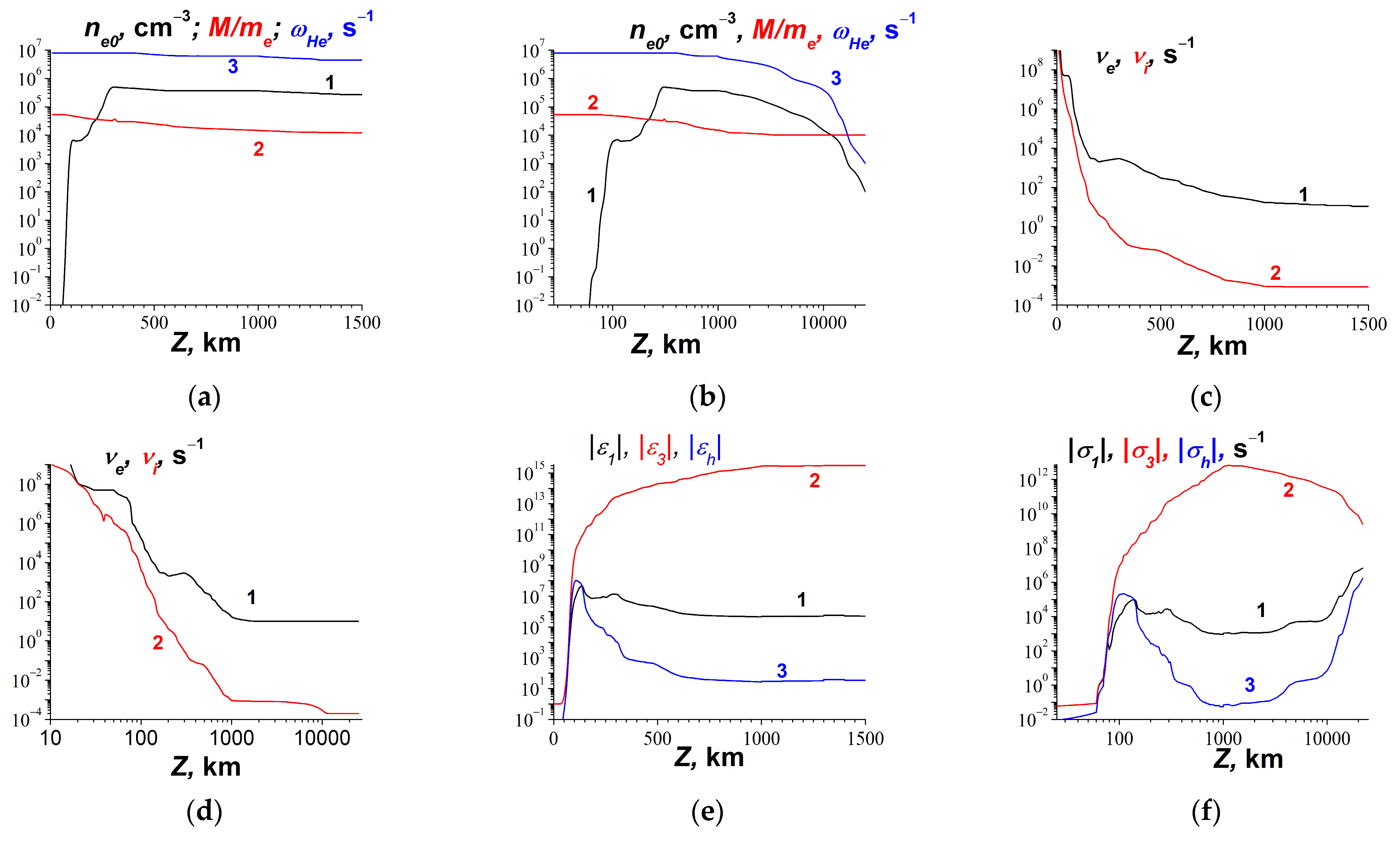
In (3), (4) $M_i,m_e,n_{e0},{\omega }_{pe,pi},{\omega }_{He,Hi},{\nu }_{e,i},H_0$ are the masses of the positive ion and electron, the concentration of electrons, the plasma frequencies of electrons and positive ions, the cyclotron frequencies of electrons and positive ions, the collision frequencies for electrons and ions, and the value of the geomagnetic field, respectively. These values depend on the height i.e., on the local vertical coordinate z. Corresponding dependencies used in modelling are shown in Section 3 (Figure 4). Hereafter, for convenience, we omit the designation of functional dependency on the height and frequency for components of dielectric permittivity tensor. The parameters of the atmosphere and the ionosphere are assumed as unchanged during the observation time. The characteristic time of essential change of the atmosphere and ionosphere parameters is of about several (3–5) hours, respectively. Frequency domain presentation is used in our paper approximately for the evaluations of the effects of electric field penetration into the ionosphere, by the order of value. We restrict ourselves by the consideration of the penetration of the electromagnetic (EM) fields from given external current sources and under given ionosphere parameters. For the other parameters, the results concerning the penetration of the electric field into the ionosphere would change, respectively.

In the coordinate frame associated with the Earth’s surface, the expression for the dielectric permittivity tensor is obtained, using (2) by rotating the coordinate frame in the XOZ plane:

$$\widehat{\epsilon }(\omega ,z)=\left(\begin{array}{l}{\epsilon }_{11}{\epsilon }_{12}{\epsilon }_{13}\\ {\epsilon }_{21}{\epsilon }_{22}{\epsilon }_{23}\\ {\epsilon }_{31}{\epsilon }_{32}{\epsilon }_{33}\end{array}\right).$$

(5)

In relation (5), ${\epsilon }_{ij};i,j=1,2,3$ are the components of the dielectric permittivity of the ionospheric plasma.

When deriving the relations for the atmosphere and the lower part of the ionosphere, the Cartesian coordinate frame is used, where the OZ axis is directed vertically upwards (Figure 1). When considering the propagation of electromagnetic fields in the upper atmosphere and magnetosphere, a set of local Cartesian coordinates associated with geomagnetic field lines within the magnetosphere is used. The approximation is that the coordinate frame is considered to be locally Cartesian, with environmental parameters that change slowly depending on the height or distance along the geomagnetic field line. The local orientation of the OZ axis is directed along the geomagnetic field line. This approximation, which is actually adiabatic, can be used due to the high anisotropy of the conductivity of the ionosphere and magnetosphere. In this case, the ULF magnetohydrodynamic (MHD) waves mainly propagate along the lines of the geomagnetic field.

Also, for wave perturbations in the ULF range, an attempt has been done to investigate the penetration of an electric field within the framework of a quasi-electrostatic approximation by means of an electric potential $\phi \sim \exp (i\omega t)$.

$$\begin{array}{l}\overrightarrow{E}\approx -\overrightarrow{\nabla }\phi ,i\frac{\omega }{4\pi }\overrightarrow{\nabla }\cdot (\widehat{\epsilon }(\omega ,z)\cdot \overrightarrow{\nabla }\phi )=\overrightarrow{\nabla }\cdot {\overrightarrow{j}}^{ext},\\ \widehat{\sigma }(\omega ,z)\equiv i\frac{\omega }{4\pi }(\widehat{\epsilon }(\omega ,z)-1),\\ \overrightarrow{\nabla }\cdot (\widehat{\sigma }(\omega ,z)\cdot \overrightarrow{\nabla }\phi )+i\frac{\omega }{4\pi }\Delta \phi =\overrightarrow{\nabla }\cdot {\overrightarrow{j}}^{ext}.\end{array}$$

(6)

The fundamental difference between quasi-stationary equations (6) and the corresponding electrostatic approximation equations, which were mostly used earlier, including some of our previous works, is the presence in the last equation of system (6), of the second quasi-static, term in the left part, proportional to the frequency ω. This will allow us to investigate for the first time the possibility of the above-mentioned boundary transition between the corresponding results for electric fields using dynamic and quasi-static approximations. The following periodic zero boundary conditions for the domains along x and y are used for the numerical solution of the equations: 0 < x < L_x, 0 < y < L_y. Accordingly, the fast Fourier transform (FFT) is used, and the corresponding modes are represented as follows:

$$E,H,\phi \sim \exp (-\mathrm{i}(k_{x}x+k_{y}y\left)\right).$$

(7)

In (7), $k_{x,y}$ are discrete wavenumbers of the corresponding Fourier modes, and for $E,H,\phi$ the amplitudes of the corresponding Fourier modes are meant, and the indices denoting the corresponding modes are omitted at the Fourier amplitudes. Then the system of two equations is obtained similarly to [15] for the column $\overrightarrow{F}\equiv {(E_x,E_y)}^T$. Here the superscript “T” means transposition, the Fourier components E_x,y depend on the local vertical coordinate z. This system is written in the matrix form as follows:

$$\begin{array}{l}\frac{\partial }{\partial z}({\widehat{A}}_1\frac{\partial \overrightarrow{F}}{\partial z})+\frac{\partial }{\partial z}({\widehat{B}}_{01}\overrightarrow{F})+{\widehat{B}}_{02}\frac{\partial }{\partial z}(\overrightarrow{F})+{\widehat{B}}_F\overrightarrow{F}+\\ +\frac{\partial }{\partial z}(\frac{1}{{\epsilon }_{33t}}{J}_z^{ext}){\overrightarrow{B}}_{1J_z}+{\widehat{B}}_{2J_z}{J}_z^{ext}{\overrightarrow{e}}_F+B_{J_{tg}}{\overrightarrow{J}}_{tg}=0.\end{array}$$

(8)

The matrices ${\widehat{A}}_1,{\widehat{B}}_{01},{\widehat{B}}_{02},{\widehat{B}}_F,{\widehat{B}}_{2J_z}$ the vectors ${\overrightarrow{B}}_{1J_z}$, ${\overrightarrow{e}}_F$, and the values $B_{J_{tg}}=-\frac{4\pi i{k}_0}{c}$, ${\epsilon }_{33t}$ included in dynamic Equation (8) are presented in Appendix A (see Equations (A12)–(A17)) along with other details of the derivation of this equation. The dependencies of the matrix and vector coefficients on ω, z are omitted in Equation (8).

It is assumed in the numerical modeling that the source of external current in the lower atmosphere has only vertical component (${\overrightarrow{J}}_{tg}=0$)

$$j^{ext}(x,y,z)\equiv j_{{}^z}^{ext}=j_0\exp [-\frac{(x^2+y^2)}{r_0{}^2}-\frac{{(z-z_1)}^2}{z_0{}^2}].$$

(9)

In relation (9), $j_0,r_0,z_{1,0}$ are the amplitude of the vertical component of the external current, the characteristic scale of the external current in the horizontal plane, the altitude position of the external current maximum, the characteristic scale of the external current in the vertical plane, respectively. Denote $L_{x,y}$ the distance between the imaginary side walls (Figure 1), which determines the periodicity of the system in the horizontal plane. Note that the boundary condition with a zero value of the tangential electric field on the imaginary sidewalls correspond to the case of a strongly localized value of the current density j_z, and the condition must be satisfied

$$r_0<<L_{x,y}.$$

(10)

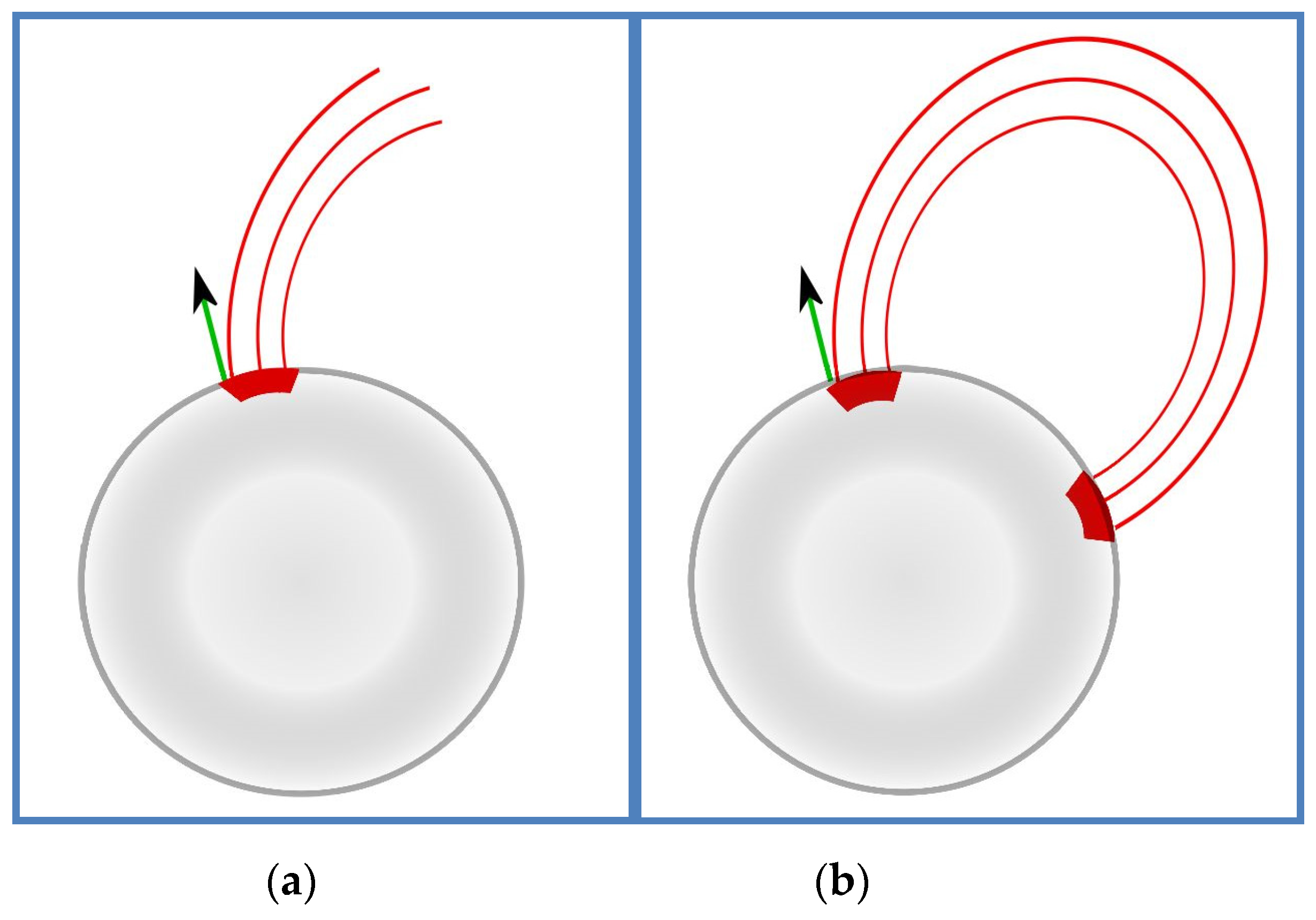
We illustrate two physically different situations mentioned above in Figure 2. The first physical situation is with geomagnetic lines which go to the magnetosphere and do not return to the Earth (open geomagnetic field lines, Figure 2a). Boundary conditions are formulated in the magnetosphere at z = L_z; these are the conditions of radiation and the absence of waves propagating in the reverse direction to the ionosphere from the magnetosphere. These boundary conditions are equivalent to a system of linear relations between dE_x/dz, dE_y/dz, and E_x, E_y analogously to [15]:

$$\frac{d{E}_x}{dz}+m_{11}{E}_x+m_{12}{E}_y=0;\frac{d{E}_y}{dz}+m_{21}{E}_x+m_{22}{E}_y=0$$

(11)

or

$$\frac{d\overrightarrow{F}}{dz}+\widehat{m}\cdot \overrightarrow{F}=0$$

(12)

Note that the matrix $\widehat{m}$ included in the left side of Equation (12) consists of elements $m_{ij};i,j=1,2$ that are included in the left sides of Equation (11).

The coefficients $m_{ij},i,j=1,2$ included in system (11) (or, (12)) are presented in Appendix A, see relations (A38). In Appendix A, the derivation of the expressions for $m_{ij},i,j=1,2$ mentioned above has been realized based on the approximation ${\epsilon }_3\to \infty$ (see relation (A18)). Nevertheless, we are interested in the comparison between the results based on the dynamic and quasi-static approaches for the determination of the electric field penetration through the system LEAIM. So, it would be quite reasonable to consider the boundary conditions (11), (12) using the more exact approach and accounting for the existence of effectively at least two small parameters in the theory describing ULF waves in the upper ionosphere and magnetosphere. One of these parameters describes anisotropy and is small in the F region of ionosphere and magnetosphere and is equal to

$$|{\epsilon }_1|/|{\epsilon }_3|(\frac{1}{{\cos }^2\theta }\frac{k_x^2}{k_t^2}+\frac{k_y^2}{k_t^2})<<1$$

(13)

where

$$k_t=\sqrt{k_x^2+k_y^2}\sim L_{\perp }^{-1}.$$

(14)

In (14), $L_{\perp }$ is the characteristic size of the transverse distribution of the (horizontal) electric field components; the determination of $k_t$ corresponds also to one presented after Equation (A10) in Appendix A. The other parameter is $|{\epsilon }_1|(k_0^2/k_{{}_t}^2)$, where $k_0=\omega /c$, and is proportional to ω, when ω is relatively small (see relation (3)).

As it follows from the accurate analysis of the Equations (A25)–(A27), the dispersion relation for Alfven waves (AWs) takes the form:

$$A_0{k}_z^2+2B_0{k}_z+C_0=0;k_{z1,2}=A_0^{-1}[-B_0\pm \sqrt{B_0^2-A_0{C}_0}].$$

(15)

In Equation (15),

$$\begin{gathered} A_0={\cos }^2\theta +\frac{{\epsilon }_1}{{\epsilon }_3}{\sin }^2\theta ;B_0=-k_x\cos \theta \sin \theta (1-\frac{{\epsilon }_1}{{\epsilon }_3}); \\ {C}_0=k_x^2({\sin }^2\theta +\frac{{\epsilon }_1}{{\epsilon }_3}{\cos }^2\theta )+\frac{{\epsilon }_1}{{\epsilon }_3}{k}_y^2-k_0^2{\epsilon }_1. \end{gathered}$$

(16)

Accounting for (13), one can get, using (15), (16), more accurate expression than (A29) for AW mode:

$$\begin{array}{l}{k}_{za}\approx k_x\tan \theta (1-\frac{{\epsilon }_1}{{\epsilon }_3}\frac{1}{{\cos }^2\theta })\\ \pm \frac{1}{\cos \theta }(1-\frac{{\epsilon }_1}{{\epsilon }_3}{\tan }^2\theta )\sqrt{k_0^2{\epsilon }_1-\frac{{\epsilon }_1}{{\epsilon }_3}(\frac{k_x^2}{{\cos }^2\theta }+k_y^2)}.\end{array}$$

(17)

The dispersion relation for fast magnetosonic waves (FMSW) mode has nevertheless the same form as the one presented in Equation (A30):

$$k_{zs}=\pm \sqrt{{\epsilon }_1{k}_0^2-k_t^2}.$$

(18)

Consider two cases, corresponding to the different ratios between the two parameters mentioned above. Namely, the first of them describes the anisotropy (see relation (13)). The second one is $|{\epsilon }_1|(k_0^2/k_{{}_t}^2)$ and is small and proportional to ω for relatively small frequency, as mentioned above.

(1) In the first case, suppose that both parameters are small, and the condition

$$|{\epsilon }_1|\frac{k_0^2}{k_t^2}<\frac{|{\epsilon }_1|}{|{\epsilon }_3|}(\frac{1}{{\cos }^2\theta }\frac{k_x^2}{k_t^2}+\frac{k_y^2}{k_t^2})<<1$$

(19)

is satisfied. Under the condition (19), Equations (17) and (18) reduce to

$$k_{za}\approx k_x\tan \theta \pm \frac{1}{\cos \theta }\sqrt{k_0^2{\epsilon }_1-\frac{{\epsilon }_1}{{\epsilon }_3}(\frac{k_x^2}{{\cos }^2\theta }+k_y^2)};k_{zs}=\pm i{k}_t.$$

(20)

Accounting for (20) and applying the approach similar to the one used in Appendix A for the derivation of the relations (A38), one can get, by the order of value, the estimation

$$\Delta z_{eff}\sim k_t^{-1}\sim L_t.$$

(21)

In relation (21), $\Delta z_{eff}$ is the penetration depth of the MHD waves penetrating into the higher ionosphere/magnetosphere from some altitude $z$ where the (horizontal) electric field distribution has the typical transverse size of order $L_t$.

(2) In the second case, suppose that, instead of (19), the second parameter $|{\epsilon }_1|(k_0^2/k_{{}_t}^2)$ is of order 1, the following condition is satisfied:

$$\frac{|{\epsilon }_1|}{|{\epsilon }_3|}(\frac{1}{{\cos }^2\theta }\frac{k_x^2}{k_t^2}+\frac{k_y^2}{k_t^2})<<|{\epsilon }_1|\frac{k_0^2}{k_t^2}\sim 1.$$

(22)

In this case, the relations (17), (18) reduce in accordance with the relations (A29), (A30), to the form

$$k_{za}\approx k_x\tan \theta \pm \frac{k_0\sqrt{{\epsilon }_1}}{\cos \theta };k_{zs}=\pm \sqrt{{\epsilon }_1{k}_0^2-k_x^2}.$$

(23)

Let us make the estimation for $z={200}^{}\mathrm{km}$, $\omega \sim 2.5\cdot {10}^{-2}{\mathrm{s}}^{-1}$, $|{\epsilon }_1|\sim {10}^7$, $L_t\sim 4000 \mathrm{km}$ (see Figures 4e and 5a,b, respectively, shown below in the Section 3). Using the relations (23), (A38), one can get

$$\Delta z_{eff}\sim \sqrt{|{\epsilon }_1|}{k}_0\sim {3000}^{}\mathrm{km}.$$

(24)

The second physical situation is when geomagnetic lines return to the Earth’s surface (closed geomagnetic field lines, Figure 2b). In this situation, the boundary conditions are E_x = E_y = 0 on the Earth’s surface (or φ = 0, for a quasi-electrostatic approximation; in the case of open geomagnetic field lines in this approximation, the same boundary condition applies to the magnetosphere). Such boundary conditions on the Earth’s surface correspond to the infinite conductivity of the Earth. The consideration of the finite conductivity of the solid Earth weakly changes the corresponding results, as our simulations have demonstrated.

For the solution of set of Equations (8) the matrix run method, or matrix factorization method [48,49,50], is used. The corresponding boundary condition (11) (or (12)), as well as zero conditions for x- and y-components of the electric field on the side walls (see Figure 1) and the lower boundary z = 0 are taken into account. This method is described in Appendix B. When the transverse sizes of the simulation region are quite large, the results of simulations are the same both for the zero boundary conditions at the sidewalls and for the periodic boundary conditions.

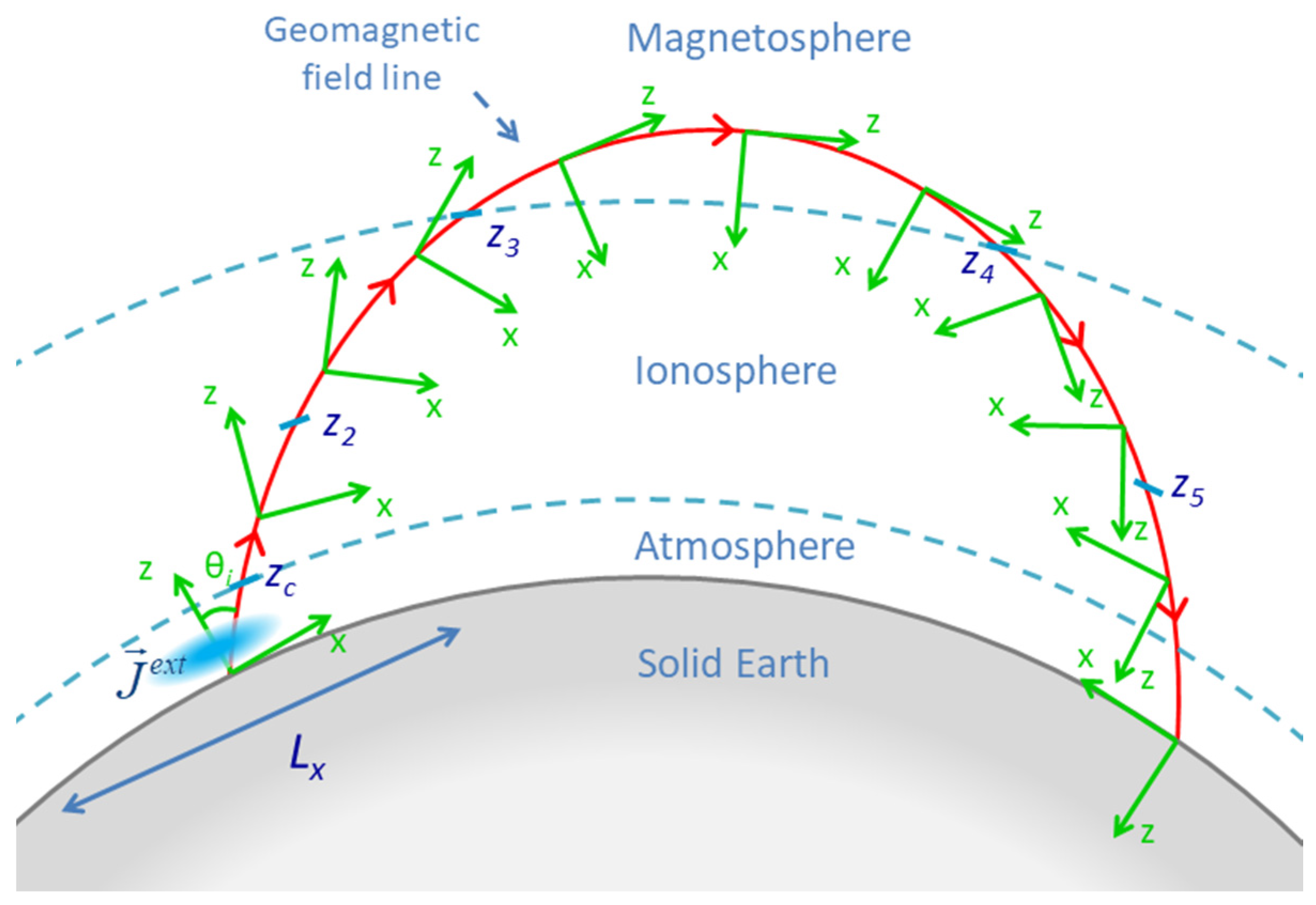
Because in the upper ionosphere and the magnetosphere the electromagnetic field propagates along the geomagnetic field lines, which are curved, the adiabatic rotation of the locally rectangular coordinate frames (c.f.) has been applied, Figure 3. Namely, near the Earth’s surface OZ axis of c.f. is aligned vertically, whereas OX, OY ones are tangential to the Earth’s surface. Starting from the altitude z = z₂ ≈ 300 km, the adiabatic rotation of OZ, OX axes takes place, and at the altitude z = z₃ ≈ 600 km OZ axis becomes aligned along the geomagnetic field line. The adiabaticity is due to the small rotation angle at each simulation step along OZ axis h_z < 1 km. In the case of open geomagnetic field lines, the OZ axis of the local c.f. preserves this orientation within the magnetosphere. In the case of the closed geomagnetic field lines, the inverse procedure has been realized near the return point, so in the return point at the Earth’s surface, OZ axis is aligned vertically. It has been checked that the simulation results depend weakly on the positions of the points z₂, z₃, z₄, z₅.

The necessity of the application of the dynamic simulations for the problem of the penetration of the electric fields into the ionosphere is due to the following factors.

1. The atmosphere, ionosphere, and magnetosphere jointly with the current sources are principally dynamic. Especially, the increase of the electric fields in the atmosphere lasts for several minutes. The properties of the ionosphere change for several hours. The conductivity of the air near the Earth’s surface is low: σ < 10⁻³ s⁻¹, so it is necessary to take into account the influence of the nonzero frequency there, if $\omega >{\omega }_{00}$; ${\omega }_{00}\sim 3\cdot {10}^{-3}{\mathrm{s}}^{-1}$.

2. When the boundary condition for the electric potential is in the deep magnetosphere L_z = 25,000 km, the deep magnetosphere itself is a dynamical system due to the Earth’s rotation around the Sun. During 1 hour of rotation, the Earth moves >100,000 km in space, so the configuration of the geomagnetic field changes.

3. In the set of papers, in particular in [45], it was shown that there are definite restrictions for the applicability of the electrostatic approximation. Further transition to the quasi-static model [46] confirms the importance of accounting for the non-stationary character of the processes in the near-Earth space. In [46], it was stated that the cases of open and close (see Figure 2 in that paper) geomagnetic field lines should be treated differently. As it is shown in Appendix C for the open geomagnetic field lines, the upper boundary conditions (relations (A53)) have the structure similar to those of the upper boundary conditions [47].

In papers [17,45,47] there were estimations of limited validity of the electrostatic approximation. Then a lot of authors used a more correct term ‘the quasi-statics’ instead of ‘the electrostatics’, for instance [46] and references there.

In the paper [46], there is a clear understanding that under different configurations of the geomagnetic field lines the approaches to simulations on the penetration of the electric field with the quasi-statics should be different, especially with respect to the boundary condition from above, see for instance Figure 2 in [46].

3. The Results of Simulations

The main goal is to estimate the penetration of the electric field components to the E- and F-layers of the ionosphere under different geometries of the geomagnetic field lines.

The values of the parameters for simulations have been selected due to the considered problem as follows. As for the height z = z₁, at which the maximum of the external current is placed, we consider two examples. In the first of them, the current maximum is somewhat raised directly above the surface region. This study is of interest from several points of view. First, the external current in the model adopted in this work qualitatively corresponds to the effective sources associated with synergetic processes. From the point of view of the prospects of the above-mentioned synergetic approach, one should take into account the presence of a number of different instabilities at different heights in the “lithosphere-ionosphere” system, including the lower atmosphere, as well as its surface layer [42,43], the mesosphere [39], E [53] and F [1,15,33] regions of the ionosphere. Therefore, it is of interest to consider the case when the external current is raised directly above the surface layer. It should be mentioned that powerful surface sources causing a noticeable response in the ionosphere include also tropical cyclones and typhoons [1,15,33,53,54,55,56,57]. The kinetic energy carried by tropical cyclones is comparable to the energy of powerful earthquakes, so the tropical cyclones are among the most destructive large-scale atmospheric formations on our planet [54,56,57]. The impact of a tropical cyclone on the ionosphere is carried out by means of a mixed mechanism, including enhanced ionization, electrophysical, hydrodynamic, meteorological, and other processes. As a result of these processes, the self-organized powerful atmospheric formation is formed, namely, an atmospheric vortex. Such a vortex is a known characteristic feature of tropical cyclone. This formation has a horizontal scale of the order of hundreds to thousands of kilometers [54]. Such a formation includes structures with strong convection and clouds, so-called convective towers [58], where both forming AGWs and intense currents and fields arising due to charge separation are clearly manifested, in particular, in lightning discharges. Moreover, such electrically saturated convective structures reach heights of 16 km [59,60]. The resulting electric fields, together with AGW, affect the ionosphere, causing noticeable disturbances of the total electron content (TEC) [58], variations in the penetration frequency foF2 [61], variations in the characteristics of VLF waves propagating in the waveguide Earth-Ionosphere and other phenomena, some of which are considered now, in the processes of tropical cyclone/hurricane formation, as the corresponding precursors [62].

In accordance with the pointed above features, for the first part of simulations, it has been adopted that the electric current source is localized in the lower atmosphere, z₁ = 14 km, above the Earth’s surface. The maximum value of the density of electric current j₀ = 0.1 μA/m², [54,56], the transverse and vertical scales r₀ = 500 km [54,56], and z₀ = 7 km [59,60] are adequate parameters, characterizing the external current source for the evaluations by the order of value.

After the calculation for a source in the lower atmosphere with an elevated maximum (z₁ = 14 km), a number of calculations will also be performed for different positions of the maximum of the external current source along with the height in the region $0\le z_1\le z_{01}$, $z_{01}=14\mathrm{km}$. Among these calculations, some will be done for the vertical coordinate of the current source maximum, which, altogether with other parameters, would qualitatively correspond to the seismogenic source. Also, calculations based on the dynamic and quasi-electrostatic approaches will be performed for some frequencies in the ULF range, with the justification for the choice of these values.

The parameters of the atmosphere, ionosphere, and magnetosphere used in the simulations for different values of height are presented in Figure 4. The parameters of the ionosphere used for modeling are taken from [18,51,52,63,64,65]. The simulations are tolerant to changes in the parameters and mainly yield qualitative results.

The choice of the frequencies of the external current source located in the lower atmosphere is due to the following considerations.

(1) We compare calculations based on dynamic and quasi-electrostatic models of electric field penetration into the ionosphere and magnetosphere. In particular, we are interested in the lower frequency limit. The frequency $\omega =2.5\cdot {10}^{-2}{\mathrm{s}}^{-1}$ chosen for the calculations determines the lower frequency limit that we can practically reach at the moment in the calculations on the basis of the dynamic model. This limit is determined by the fact that decreasing model frequency two times requires a fourfold increase in Random Access Memory (RAM), during the calculations based on the dynamic approach. Despite this, we qualitatively investigate the penetration of the field into the ionosphere and magnetosphere also at frequencies $\omega <2.5\cdot {10}^{-2}{\mathrm{s}}^{-1}$ for the quasi-electrostatic approach.

As shown below, the application of the quasi-electrostatic approach is adequate for the case of closed geomagnetic field lines. Moreover, the goals of this work include clarifying the qualitative nature of the dependences of the field penetration on some parameters of the source, including its frequency. The calculation results in the dynamic and quasi-electrostatic approximations are compared in the region of minimum frequencies $\omega \sim 2.5\cdot {10}^{-2}{\mathrm{s}}^{-1}$ (namely, for $\omega =2.5\cdot {10}^{-2}{\mathrm{s}}^{-1}$ and $\omega =5\cdot {10}^{-2}{\mathrm{s}}^{-1}$), in which our computational capabilities still allow us to apply not only the quasi-electrostatic approximation, which does not have, with the mathematical point of view, frequency restrictions “from below”, but also a dynamic approach.

As we will demonstrate in this section, in the aforementioned boundary frequency range, where both dynamic and quasi-static approaches are applicable, they, as expected, with appropriate calculations, give for the maxima of the field components the values of the same order of magnitude. In our qualitative studies of the electric field penetration from the lower atmosphere into the ionosphere and magnetosphere, the accuracy of determining the field components in order of magnitude is quite satisfactory.

(2) Let us take into account the existence of a correspondence, as will be shown below, in order of magnitude and in qualitative behavior depending on the height, between the results obtained in the case of closed geomagnetic field lines for the maximum field value using dynamic and quasi-electrostatic approaches. This allows, by matching the results for these two approaches in the above-designated frequency range, where they are both applicable, to “go down” in frequency on the basis of a quasi-electrostatic approach. Thus, it is possible to study the field penetration from a given (external) current source, with an accuracy of an order of magnitude, in the lower part of the ULF range.

The typical results of simulations are presented in Figure 5, Figure 6, Figure 7, Figure 8, Figure 9 and Figure 10. The frequency interval is ω = 0.025–0.05 s⁻¹, where there is a possibility to apply the quasi-electrostatic approximation. The values of the electric field components are in mV/m units. The results of the simulations are of qualitative character and are tolerant to changes in the parameters of the ionosphere. The region of simulations in the locally horizontal plane XOY has been chosen quite large to avoid an influence of boundaries on the electric field distributions, so it should be L_x,y ≥ 10,000 km. The initial inclination of the geomagnetic field from the normal to the Earth’s surface is θ_i = 10°. The results depend weakly on this parameter when θ_i < 30°.

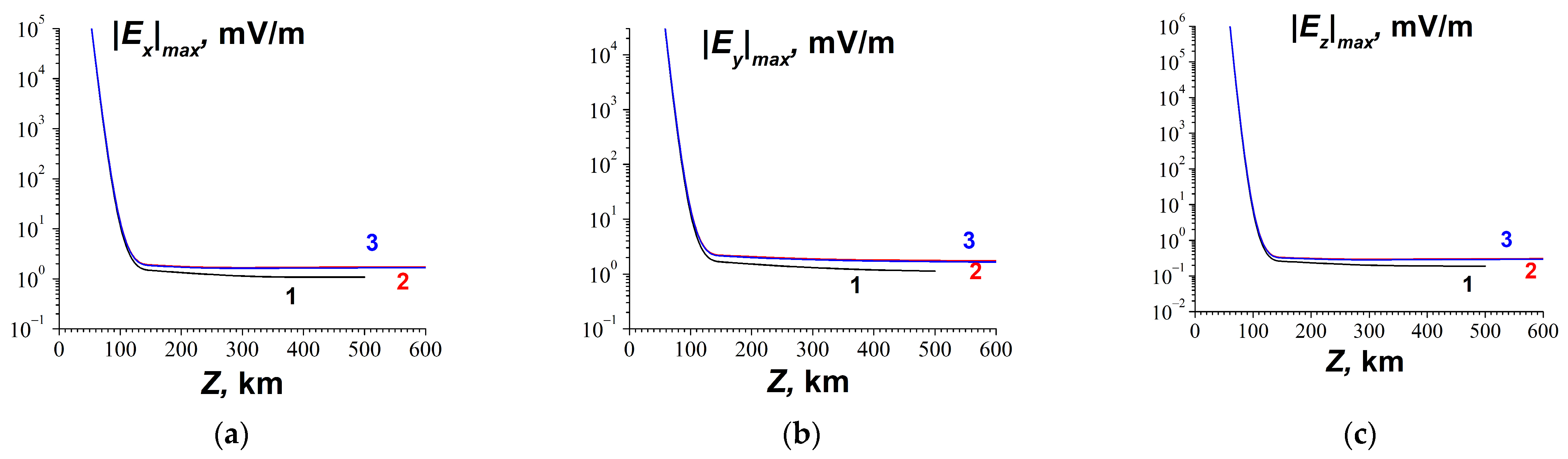
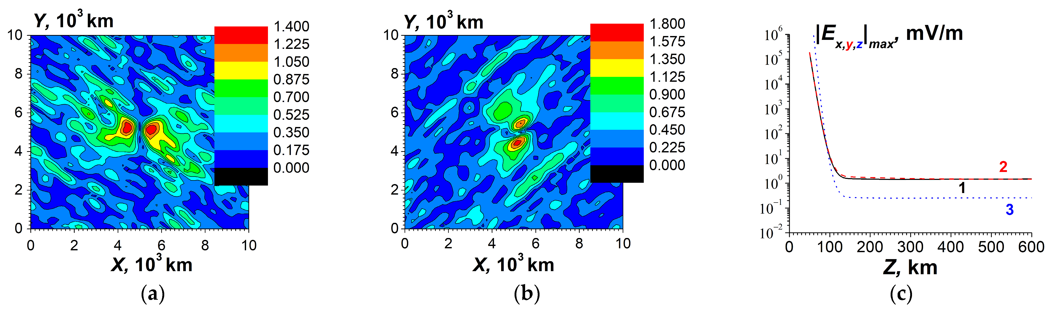
In the case of open field lines, the results of simulations are presented in Figure 5, Figure 6, Figure 7 and Figure 13. Within the dynamic simulations there exists the penetration of the horizontal electric field components to the heights z > 150 km. These dependencies are presented at the heights z ≥ 50 km only because at lower heights the values of the electric field, especially the vertical component E_z, cannot be computed correctly in the regions where the external current source j^ext is not zero [15]. The used approximation of the given external current sources is too rough there [15]. Within the dynamic approach, the simulated penetration does not depend on the position of the upper boundary condition L_z, when L_z ≥ 1000 km, see Figure 5. Specifically, the dependencies for the upper boundary condition at L_z = 25,000 km coincide with ones for L_z = 1500 km, curves 3 in Figure 5. 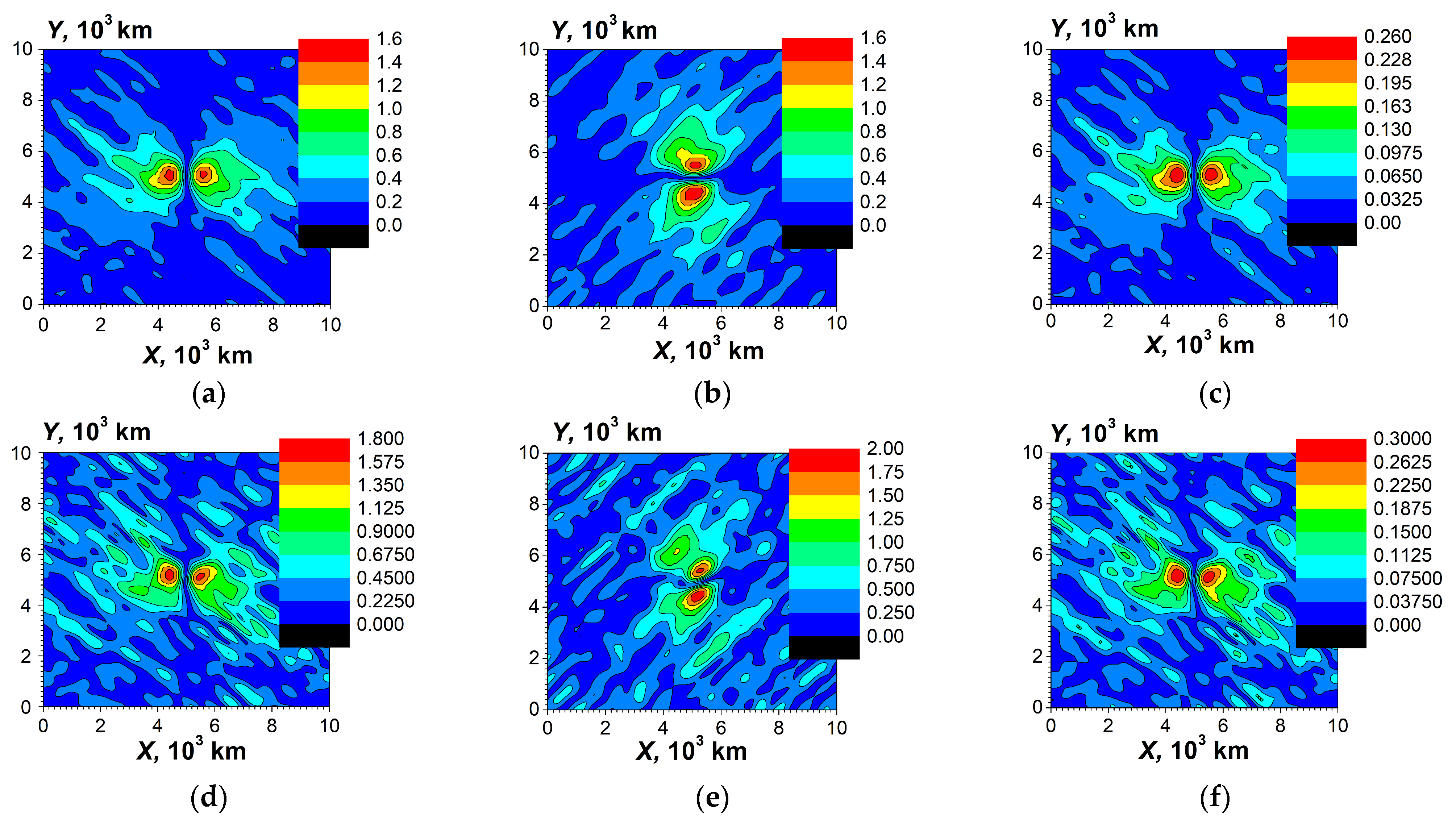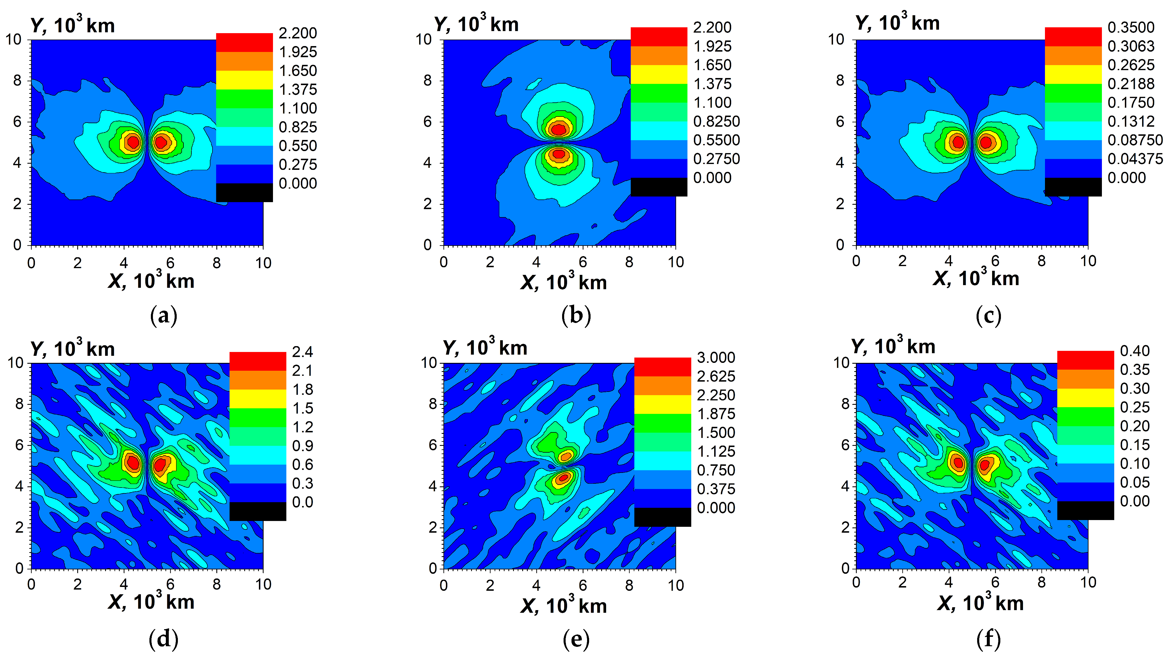Also, the values of the electric field components depend slightly on the frequencies at ω ≤ 0.1 s⁻¹. This can be seen from Figure 6 where the spatial distributions of the electric field components are presented at z = 200 km in F-layer; compare Figure 6a,d (for E_x component), Figure 6b,f (for E_y component), and Figure 6c,g (for E_z component). Moreover, in the dynamic simulations for the open geomagnetic lines, the results of simulations with the adiabatic rotation of the coordinate frame (c.f.) coincide with ones without such a rotation, where the orientation of c.f. has been unchanged.

Note that under the parameters used for the modeling presented in Figure 5 and Figure 6, the evaluation (24) is suitable and corresponds qualitatively to the results presented in the Figures mentioned above. The difference of frequency in two times leads to a difference in maxima of amplitudes of electric field components which does not exceed a value of order (compare Figure 6a–c with Figure 6d–f, respectively). In the accordance with (24), in the magnetosphere at the vertical distances z > 1000 km, the maxima slowly decrease with the growth of z, as our simulations have demonstrated, but the detailed investigation of the penetration of the electromagnetic fields into the magnetosphere is out of scope of this paper.

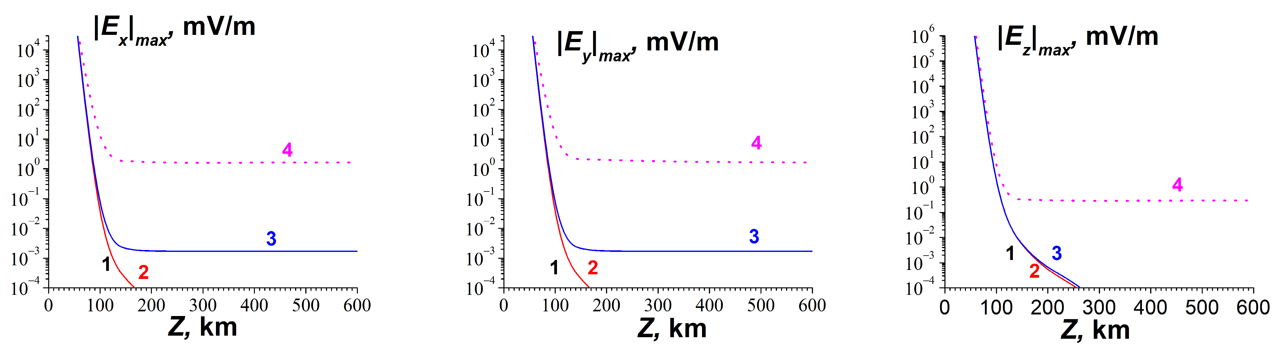
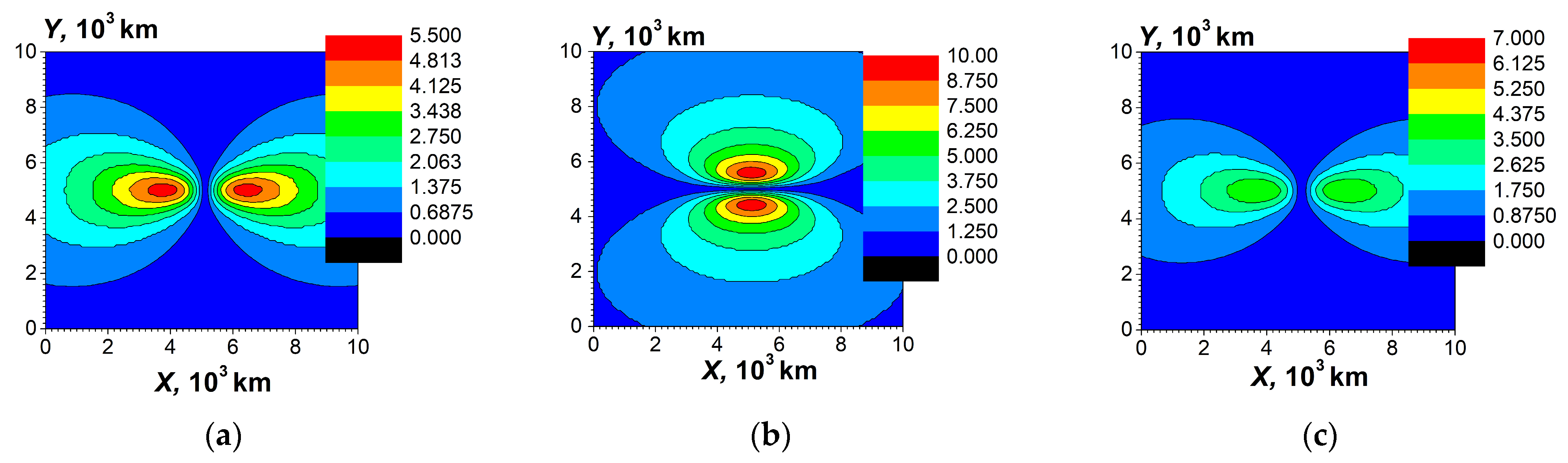
Contrary to this, within the quasi-electrostatic approximation the simulated penetration is very poor in the ionosphere F-layer, 3 orders smaller than one within the dynamic simulations. The results of the quasi-electrostatic simulations are given in Figure 7. Two types of boundary conditions within the magnetosphere have been applied, namely either φ = 0 or E_z = 0. The results of the simulations do not depend on the types of the boundary conditions. Note that the upper condition E_z = 0 corresponds to the absence of the electric current along the geomagnetic field line [46]. The simulated values of the electric field depend on the position of the upper boundary condition. For the curve 1 the value of L_z is L_z = 1000 km, for curves 2, 3 they are 1500 km and 25,000 km (Figure 7). At the distance L_z = 25,000 km along the geomagnetic field line, i.e., in the deep magnetosphere, the parameters of the magnetosphere are assumed as n_e0 = 10² cm⁻³, M/m_e = 10⁴, ω_He = 10³ s⁻¹, ν_e = 10 s⁻¹, ν_i = 10⁻⁴ s⁻¹, that yields the components of the conductivity σ₁≈ 3.1·10⁵ + i6.8·10⁶, σ₃≈ 2.6·10⁹ − i1.1·10⁸, σ_h ≈ −1.7·10⁶ + i2.9·10⁴. The results of the quasi-electrostatic simulations depend weakly on changing the parameters in the deep magnetosphere.

The explanation of the great difference between the results of the dynamic and the quasi-static approximations (compare Figure 5a–c and Figure 7a–c, respectively) is as follows. The quasi-electrostatic approximation can be applied when the following condition of the small retardation is valid: L_z << v_A/ω [66], where v_A = c/ε₁^1/2 ≈ H₀/(4πn_e0M)^1/2 is the Alfven velocity [51,52]. For the rough estimations we accept the condition of the validity of quasi-electrostatic approximation in the form:

$$L_z<\frac{v_A}{2\omega }.$$

(25)

It is of about v_A ≈ 400 km/s within the upper ionosphere and v_A ≈ 100 km/s in the magnetosphere [51,52]. Thus, it should be L_z < 2000 km. Such a condition could not be satisfied for L_z = 25,000 km, see curves 3 in Figure 7a–c, built for the open field line and quasi-electrostatic. In the case of open geomagnetic field lines, it is seen from Figure 7 that the behavior of the electric field depends essentially on the position point L_z of the upper boundary condition, compare curves 1, 2, and 3 in Figure 7. Within the quasi-electrostatic approximation at all values of L_z the electric field in the ionosphere, F-layer is several orders smaller compared with the dynamic simulations, Figure 5.

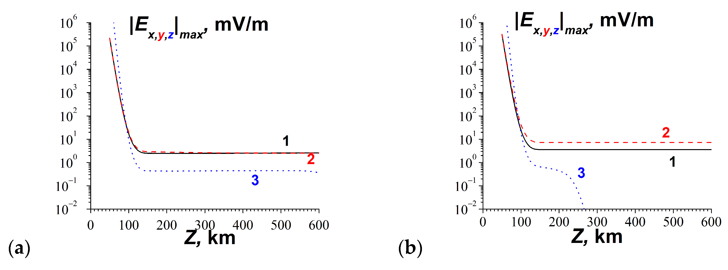
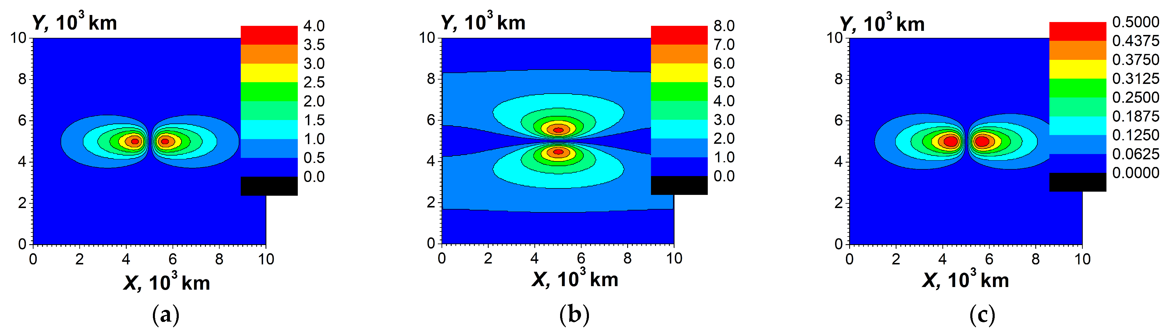
In the case of closed geomagnetic field lines, the horizontal components of the electric field penetrate into the ionosphere both within the dynamic simulations and in the quasi-electrostatic approximation. The results of simulations are given in Figure 8, Figure 9, Figure 10, Figure 11 and Figure 12. The distance along the geomagnetic field line is L_z = 2000 km, i.e., it includes two parts, from the Earth’s surface to the magnetosphere and back from the upper point in the magnetosphere to the Earth’s surface. The values of the electric field have a correspondence in these simulations. The quasi-static approximation is approximately valid, when the total distance along the geomagnetic field line is of about 2000 km between the Earth’s surfaces. The quantitative difference is due to both some non-quasi-stationarity and the roughness of the model. In this case, to get more exact results it is necessary to take into account in detail the curvature of the geomagnetic field lines under the quasi-static approximation. Under dynamic simulations, the influence of this curvature is not so essential, as our simulations have been demonstrated.

As it is seen from Figure 9, parts a and d, b and e, c and f, in the case of closed geomagnetic field lines, the differences in corresponding maximum values of electric field components for the frequencies 0.05 s⁻¹ and 0.025 s⁻¹ does not exceed a value of order 25%.

From Figure 5 and Figure 8 it is seen that the dynamically computed values of the electric field in the ionosphere F-layer are a bit higher in the case of closed geomagnetic field lines. This can be explained by a partial reflection of the magnetohydrodynamic waves from the Earth’s surface in the place of returning the geomagnetic field lines.

Our simulations have been demonstrated that for the quasi-electrostatic simulations when the inclination angle is θ_i > 10°, the distributions become smeared in the horizontal plane. This numerical effect does not change the results qualitatively; it can be removed accounting for the curvature of the geomagnetic field lines, using a curvilinear coordinate frame. Also, the tuning of the locally horizontal region of simulations in the upper ionosphere and the magnetosphere should be realized. But there is a simpler solution to the pointed above problem [46]. Since the longitudinal conductivity, that is, the component along the geomagnetic field line, is 5–7 orders of magnitude greater than the transverse conductivity in the upper ionosphere and magnetosphere, it is possible to make a connection by short-circuiting two regions of the ionosphere, namely the one from which the geomagnetic field line comes out and the one into which this line enters, i.e., magnetically conjugated region. Thus, the corresponding ionospheric regions located at altitudes up to z = 300 km can be connected. In other words, in the quasi-electrostatic simulations, it is possible to avoid the simulations within the upper ionosphere and the magnetosphere. Of course, this procedure is valid only in quasi-electrostatic simulations in the case of closed geomagnetic field lines. In this simplified approach the results of simulations are of agreement with the dynamic simulations under greater inclination angles θ_i > 20°. The results of simulations at higher inclination angles are given in Figure 11 and Figure 12, the quasi-electrostatic and dynamic simulations correspondingly.

From Figure 11 and Figure 12 it is seen that in the case of the closed geomagnetic field lines the correspondence between the values of the penetrated electric field obtained in the dynamic and quasi-static simulations is also valid at higher inclination angles of the geomagnetic field. The maximum values of |E_y| component along the axis OY perpendicular to the geomagnetic field are practically the same in Figure 9e, and in Figure 12b, for the dynamic simulations; and in Figure 10b, and Figure 11b, for the quasi-static ones

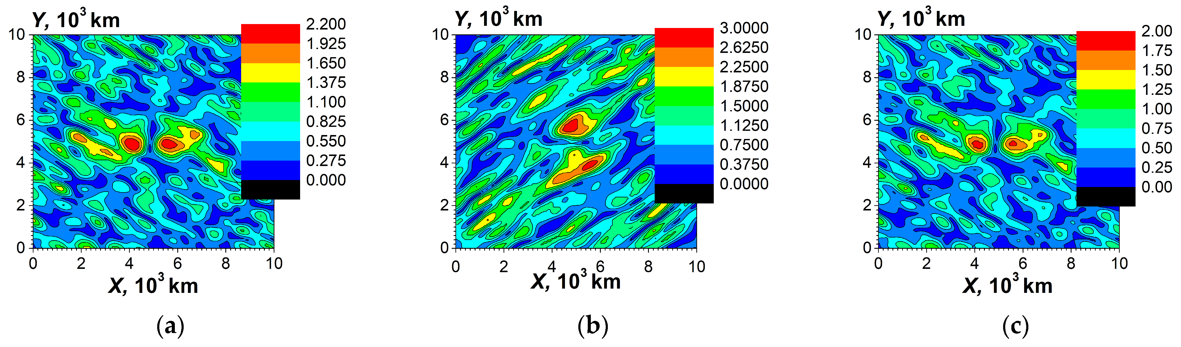
From Figure 6, Figure 9, and Figure 12 it is seen that in the horizontal distributions |E_x,y,z|(x,y) there exists the prolonged fine structure of the scales ~4000 km. This structure is more expressed at lower frequencies, compared to Figure 6 and Figure 9, parts a, b, c at ω = 0.05 s⁻¹, and parts d, e, f, ω = 0.025 s⁻¹. The main maxima are similar for all frequencies. The origin of this fine structure is due to propagation of the EM waves in the gyrotropic ionosphere and in the lower magnetosphere, z ≤ 600 km, which are strongly non-uniform in the vertical direction. The strong coupling between outgoing waves and backward ones occurs there. Such interference is more essential at lower frequencies where the longitudinal wave numbers are smaller. Our simulations have demonstrated that at higher frequencies ω > 0.05 s⁻¹ this prolonged structure is practically absent. The prolonged structures are less pronounced at inclination angle θ_i = 40^o (Figure 12a–c) than at θ_i = 10° (Figure 9d–f). The details of forming this structure should be a subject of special investigations, especially at lower frequencies ω < 0.025 s⁻¹.

At lower frequencies ω < 0.025 s⁻¹ the utilized algorithm for the dynamic simulations needs the extremely large amount of the computer memory, namely the decrease of the frequency two times demands the increase of the memory at least four times, i.e., the doubling of the points along both OX and OY axes. The reason is that the field components E_x, E_y are used as independent functions under the dynamic simulations and the transition to the exactly static case ω → 0 is a non-trivial computation problem. In the quasi-static simulations, the single function φ is used at all frequencies and the problem pointed above is absent.

The dependencies of the maximum values of the electric field components on the position of the external current have been simulated. A dynamic approach was used for the cases of open and closed field lines (see the first and second lines in

Table 1. The dependencies of the maximum values of |E_x|, |E_y|, |E_z|, mV/m, on the position of the excitation current z₁, the circular frequency is ω = 0.025 s⁻¹. The inclination angle of the geomagnetic field is θ_i = 10°. There are the same parameters z₀ = 7 km, j₀ = 0.1 μA/m²; x₀ = y₀ = 500 km, besides the data in the last column of the table.

z1, km	14	10	7	5	3	0	0, but x0 = y0 = 1000 km
Dynamic simulations, open lines	1.7	1.65	1.6	1.45	1.25	0.85	1.55
	2.0	2.0	1.85	1.7	1.5	1.0	1.62
	0.3	0.29	0.28	0.255	0.22	0.15	0.275
Dynamic simulations, closed lines	2.45	2.44	2.35	2.15	1.85	1.3	2.37
	2.8,	2.8	2.65	2.42	2.1	1.45	2.42
	0.43	0.43	0.41	0.38	0.33	0.23	0.42
Quasi-electrostatic simulations, closed lines	3.6	2.5	1.8	1.36	0.96	0.5	0.92
	7.3	5.1	3.6	2.7	1.93	0.99	2.0
	0.50	0.35	0.25	0.19	0.13	0.07	0.13

). It is seen that the maximum values only slightly depend on the position of the maximum external current density when this current lies in the atmosphere, z₁ ≥ z₀. Some decrease occurs when the current partially cuts of by the Earth’s surface. Additionally, in Table 1 (see the third line) there are dependencies of the maximum values of the electric field components for the closed geomagnetic lines obtained under the quasi-electrostatic simulations.

Note that the dependence on the vertical coordinate in the spatial distribution of the external current (9) with the parameters z_l = (3–5) km, z₀ = 7 km corresponds qualitatively to the distribution of seismogenic external current in [67]; transverse scale x₀ = y₀ = 500 km and 1000 km correspond to the parameters of powerful earthquakes with magnitudes M = 6.27 and 6.98, respectively [68]. As it is seen from Table 1, electric field penetrating at a given altitude in the ionosphere with the chosen parameters differ less than 1.5 times, for the cases of open and closed geomagnetic field lines, in the simulations based on the dynamic approximation.

The distributions of the electric field components are presented for the case when the external current partially is cut by the Earth’s surface, Figure 13.

It is seen that the distributions shown in Figure 13a,b are similar to ones in Figure 6d,e, respectively, while curves 1, 2, 3 in Figure 13c are similar to curves 3 in Figure 5a–c, respectively. The difference is in 15% smaller maximum values of |E_x|, |E_y| in Figure 13, due to the cut-off of the external current by the Earth’s surface.

In addition to the calculations, presented in Table 1, it was also shown that for the quasi-electrostatic case and closed geomagnetic field lines, in the frequency range 10⁻⁴ s⁻¹ ≤ ω ≤ 0.025 s⁻¹, the dependence of the maximum values of the electric field components on the frequency, at z = 200 km changes unessentially within 3% difference; this was shown, in particular, for the parameters z₁ = 14 km, z₀ = 7 km. Note also that, in the frequency range ${10}^{-4}{\mathrm{s}}^{-1}<\omega <{10}^{-3}{\mathrm{s}}^{-1}$, the calculations are rather formal and mathematical in nature. The reason is that during a time of order of the corresponding period of oscillations, $2\pi /\omega \sim 20 \mathrm{h}$ ($\omega \sim {10}^{-4}{\mathrm{s}}^{-1}$), the changes in the parameters of the atmosphere and ionosphere, ignored in the frequency domain presentation, are already quite essential.

4. Discussion

The important problem of the penetration of the electric field to the ionosphere from the near-Earth sources is under investigation till now. A standard approach is the utilization of the electrostatic or quasi-electrostatic equation for the electric potential in media with highly anisotropic conductivity supplemented by boundary conditions. At the high conductive solid Earth’s surface, the boundary condition is a constant value of the electric potential. Usually, some boundary condition for the electric potential and its derivatives is formulated at the boundary between the upper atmosphere and the lower ionosphere. But still, it has been unclear what boundary condition should be applied within the quasi-electrostatic approach in the magnetosphere and how to transfer the boundary condition to the lower ionosphere and whether such a transfer is valid. This basic problem is due to the high anisotropy of the conductivity of the upper ionosphere and the magnetosphere and mathematically is expressed through the product of a small value of the electric field along the geomagnetic field line and a very big value of the conductivity along with it, in order to calculate the density of the electric current. Thus, within the framework of the electrostatics, the correct formulation of the upper boundary condition for the electric potential is doubtful.

Nevertheless, the processes in the ionosphere and the magnetosphere are principally dynamic, so the case of the quasi-electrostatics may be justified only at small spatial scales. To perform this approximation, the condition (25) must be satisfied. The maximal period T can be estimated as T ≤ 2·10³ s, i.e., the variation time of the current sources is smaller than 1 hour. Therefore, for the validity of the quasi-electrostatics, the distance along the geomagnetic field line should be L_z < 2·10⁴ km. From this simple estimation, it is seen that in the case of the open geomagnetic lines the quasi-electrostatic approximation is doubtful, whereas for the closed geomagnetic field lines it could be valid.

Generally, the dynamic approach should be used to consider the problem of penetration of the ULF electric field to the ionosphere. The simulations within the quasi-electrostatic approximation should correspond to the results of the dynamic simulations. The dynamic method is based on the Maxwell equations and proper boundary conditions for the electromagnetic field. Because the physical processes possess various temporal scales, to make the qualitative analysis as clear as possible, it is rather better to apply the spectral approach, i.e., within the frequency domain. Our dynamic simulations have been proven that in the case of open geomagnetic field lines the quasi-electrostatic approximation does not provide adequate results. Moreover, the results of simulations obtained within the dynamic method do not depend on the position of the upper boundary within the magnetosphere when the heights are ≥1000 km, which proves the validity of the dynamic approach. The boundary conditions for the EM field are the absence of the ingoing magnetohydrodynamic waves. Contrary to this, in the case of open geomagnetic lines, the results of the quasi-electrostatic simulations depend on the position of the upper boundary condition and the penetrated electric field in the ionosphere F-layer is several orders smaller than one obtained in the dynamic simulations.

In the case of the open geomagnetic field lines, the dynamic method for the penetration of the ULF electric fields from near-Earth sources to the upper ionosphere and magnetosphere is similar to the consideration of penetration of the magnetosphere perturbations due to the solar wind to the lower ionosphere and the atmosphere. Namely, those perturbations propagate along the magnetic field line as the magnetohydrodynamic waves, and only near the Earth’s surface the quasi-static approximation is valid and used [69].

The physical reason for the significant difference between the results obtained on the basis of the dynamic and quasi-static approaches (Figure 5 and Figure 7) in the case of open magnetic field lines is as follows. In the dynamic approach, we use the radiation condition (Equations (11) or (12)) as the “upper boundary condition”. This condition is set at the heights of the upper ionosphere or magnetosphere, where, for the frequency range under consideration, inhomogeneities in the medium are so smooth on the wavelength scale that the reflection for a wave emitted from the studied area can be neglected with sufficient accuracy [70]. This condition corresponds to the principle of causality [71], in particular, in the presence of (external current) sources only in the lower atmosphere. It turns out that the field excited by a given source in the lower atmosphere and penetrating into the ionosphere and magnetosphere is negligibly dependent on the location of the boundary at which the “upper boundary condition” (of radiation) is set in the upper ionosphere or magnetosphere (see Figure 5 and its description in Section 3). As for the quasi-static approach, it is applicable, if (25) is satisfied. Obviously, in the case of open geomagnetic field lines, a similar condition is violated at a sufficiently large value of L_z, for example, at L_z = 25,000 km. This is confirmed by the corresponding modeling illustrated in Figure 7.

In addition to this, we can also offer the following visual explanation of the significant difference between the results obtained on the basis of the dynamic and quasi-static approaches. If the radiation condition under the dynamic approach is formulated at a certain value of the coordinate z = L_z1, then we can assume that at z > L_z1 there are, respectively, only waves radiated from the considered region $0\le z\le L_z$. If we now set the radiative boundary condition at $z=L_{z2}>L_{z1}$, then in both regions $L_{z1}<z\le L_{z2}$, $z>L_{z2}$, in fact, only outgoing waves will be present, since the reflection in the region $L_{z1}<z\le L_{z2}$ is negligible. Therefore, the field in the region $z<L_{z1}$, including the lower and middle ionosphere, will be practically insensitive to the location of the “upper boundary” selected in the upper ionosphere or magnetosphere (at z = L_z1 or z = L_z2). The situation is significantly different when the quasi-static approximation is used. In this approximation, there is neither delay nor radiation. As a result, when using the quasi-static approximation, the entire region $0\le z\le L_z$ automatically belongs to the “region of influence” in the solution, even at very large values of L_z. Therefore, the value L_z, which determines the place where the “upper boundary condition” is specified, significantly affects the solution when applying the quasi-electrostatic approximation. This indicates the inapplicability of the quasi-electrostatic approximation in the case of open geomagnetic field lines.

In the case of the closed geomagnetic field lines both the dynamic approach and quasi-electrostatic one yield practically similar results for the penetration of the electric field into the ionosphere F-layer. Therefore, it is natural to set the appropriate boundary conditions on the surface of the Earth, in the regions from which the geomagnetic field lines emerge and where they return. Boundary conditions are set in a similar way when using the quasi-static approximation. Both in the quasi-electrostatics and in the dynamic approach the boundary conditions are zero values of the tangential electric field on the Earth surface; in the quasi-electrostatics, they are equivalent to the zero-electric potential.

It was mentioned in [46] the difference between the pointed above configurations of the geomagnetic field lines for the electrostatic simulations and the necessity to use different boundary conditions in the lower ionosphere. The upper boundary conditions used in [46,47] correspond qualitatively and by mathematical structure to the upper boundary condition derived in the present paper, see Appendix C, Equation (A53).

In Section 3 it has been mentioned the mathematical limitation for the lowest frequency that can be used in our model of the dynamic simulations. This mathematical limitation seems not occasional and has a physical sense with respect to an attempt to “move” into the region of lower frequencies on the basis of the dynamic approach. Namely, with decreasing frequency, one should expect that the solution for the electromagnetic field can be represented in terms of electromagnetic potentials [66,71,72]. Alternatively, such a solution can be presented in terms of magnetic and electrical Hertz potentials, which in the limit of low frequencies are transformed into electrostatic and magnetostatic potentials [71]. With this approach, it is quite obvious that the solution of the dynamic problem, in principle, cannot reach the purely electrostatic limit, since in this case “the magnetostatics is lost”. In any case, this must necessarily happen in the presence of low-frequency currents in the system, as in our case. In a geophysical experiment, this corresponds to the presence of a magnetic ULF field, excited by the corresponding currents, which can be measured at ground-based and satellite observatories.

Despite the fact that in this work a different approach is used with the reduction of Maxwell equations in the frequency domain to a system of two equations of the second order (8) for the Fourier amplitudes of two transverse components of the electric field, it seems obvious that also, in this case, two corresponding functions, associated with the transverse components of the electric field, cannot in the limit tend to a single function, namely, the electrostatic potential. The aforementioned mathematical difficulty with an increase in the required amount of RAM with a decrease in the source frequency is probably a mathematical reflection of the physical problem of the transition to quasi-electrostatics and quasi-magnetostatics. In the future, it will be of interest to consider the question of the “magneto-electrostatic” limit for the electrodynamic solution in the LEAIM system.

Our dynamic simulations, supplemented by quasi-electrostatic simulations (for the case of closed geomagnetic field lines) have demonstrated that the values of the electric field are, by the order of value, of about several, namely (1–5) mV/m in the lower ULF range of frequencies (${10}^{-3}{\mathrm{s}}^{-1}\le \omega \le 5\cdot {10}^{-2}{\mathrm{s}}^{-1}$) in the ionosphere F-layer at the heights z = 200–600 km and in the lower magnetosphere. Moreover, the corresponding simulations may be done even at such low frequencies, as ${10}^{-4}{\mathrm{s}}^{-1}\le \omega <{10}^{-3}{\mathrm{s}}^{-1}$, but only formally, if one would ignore the fact, that the parameters of the atmosphere and ionosphere change essentially during the period ($2\pi /\omega \sim 20\mathrm{hours}$, $\omega \sim {10}^{-4}{\mathrm{s}}^{-1}$) of corresponding current source oscillations.

The results for the penetration of electric field into the ionosphere are obtained using the models of external current sources localized in the lower atmosphere with a maximum value of 0.1 μA/m², generated by tropical cyclones [54,56,57] or seismogenic (earthquake preparation) processes [1,6,24]. Such electric fields, by the order of value, are corresponding to the ionospheric observations above tropical hurricanes [61,73] and the region of the preparation of strong earthquakes [40]. Such values of the electric field correspond also to the observations of seismogenic variations in electron concentration and TEC [6,41]. Therefore, the simulated values of the electric field are of a qualitative agreement with the results of observations. Note also that the value of the extraneous current maximum of ~ 0.1 μA/m² accepted in the calculations in this work is far from the maximum possible corresponding value known from the literature. Namely, there are theoretical estimates that substantiate the possibility of generating external currents in the lower atmosphere with values exceeding those mentioned above by one or even two orders of magnitude. Such estimates are given, in particular, in works devoted to modeling and observations of ionospheric effects caused by electric fields from surface current sources of a seismogenic nature (during the preparation of powerful earthquakes) [6,67,74,75] and sources associated with tropical cyclones [54,56].

The external current only mimics the real current generated in the lower atmosphere by all physical processes taking place in a self-consistent manner, but at the same time, it allows one to determine the field penetrating into the upper ionosphere/magnetosphere. To adequately determine the electric field in the lower atmosphere, a synergetic approach is required with consideration of all relevant physical processes, instabilities in the LEAIM system, their nonlinear limitation [9,15,34], as well as the corresponding boundary conditions, including ones in the lower atmosphere, for various current components associated with different types of charged particles, including aerosols and ions, and taking into account photochemistry, convection, hydration and other dynamic processes [1,4,6,24,32]. The synergetic approach would include, naturally, the self-consistent investigations with accounting for positive feedback between the penetrated EM field and changes in the ionosphere parameters. This may be a subject of future works.

5. Conclusions

The penetration of an electric field through the LEAIM system is of a dynamic nature, in particular, in the presence of external current sources exciting the electromagnetic fields in the lower atmosphere or lithosphere. This dynamic nature is due to the variation in time in both properties of the atmosphere, ionosphere, and the magnetosphere and of the external sources. Also, it should be taken into account the possible propagation of electromagnetic disturbances over large distances along the geomagnetic field lines. This propagation results in retardation of the electromagnetic field. Thus, the correct formulation of the problem should be done, generally speaking, on the basis of a dynamic approach to solving the Maxwell equations.

In this case, the corresponding dynamic boundary conditions for the electromagnetic field must also be formulated correctly. The ULF waves considered in this paper propagate to a large distance along the lines of the geomagnetic field. Two essentially different situations arise: (1) the geomagnetic field lines emerging from the Earth-Atmosphere boundary in the region of the location of an external electric current source are open, passing from the upper ionosphere into the deep magnetosphere, and do not return into the ionosphere (for sufficiently high latitudes); (2) after penetration from the ionosphere into the lower magnetosphere, the geomagnetic field lines return to the magnetically conjugated ionosphere and then again fall from the atmosphere into the Earth (lithosphere). Naturally, for the electromagnetic field at the “second end” of the line of force, where the numerical calculation completes, there are significantly different boundary conditions. In the case of open field lines, this is the condition of radiation, and in the case of closed field lines, the tangential component of the electric field is equal to zero, if the conductivity of the Earth is considered equal to infinity. It turns out that in the case of open geomagnetic field lines only the dynamic approach is applicable, but the quasi-static approach is not valid, and in the case of closed geomagnetic field lines the quasi-static approximation can also be used, since it gives results that qualitatively and quantitatively, by the order of value, coincide with the results obtained on the base of the dynamic approach. In the case of closed filed lines, the electric potential calculated in the upper part of the first ionosphere (located above the region where external sources are considered) can be transferred along the geomagnetic field lines to the upper part of the magnetically conjugated ionosphere, and then it will continue the calculation, in particular, in the atmosphere magnetically conjugated region.

The values of the electric field obtained in the dynamic approximation are of about several (1–5) mV/m in the ionosphere F-layer and in the lower magnetosphere. In this case, the results are similar to ones obtained within the quasi-electrostatic approximation simulations when the geomagnetic field lines return to the Earth’s surface. In the region near the boundary between the atmosphere and the ionosphere z = 60 km the electric fields are several (1–5) V/m. The external electric current sources have a maximum value of 0.1 μA/m² and are localized in the lower atmosphere. The simulated values of the electric field are of a qualitative and even quantitative, by the order of value, agreements with the results of observations of electric fields and perturbations of the electron concentration/TEC, caused by the current developed in connection with tropical cyclones or the seismogenic processes (the preparation of the most powerful earthquakes).

Note that to the parameters used for the modeling presented in Figure 5 and Figure 6, the estimation (24) of the penetration depth appeared to be suitable and corresponds qualitatively to the results presented in the Figures mentioned above.

Numerical-analytical algorithms are given in detail, including the derivation of boundary conditions and a numerical scheme based on a combined spectral–finite difference method for dynamically modeling the field penetration from a given electric current sources in the lower atmosphere through the LEAIM system.